Digital Image
Processing
Third Edition
Rafael C. Gonzalez
University of TennesseeRichard E. Woods
MedData InteractiveVice President and Editorial Director, ECS: Marcia J. Horton Executive Editor: Michael McDonald
Associate Editor: Alice Dworkin Editorial Assistant: William Opaluch Managing Editor: Scott Disanno Production Editor: Rose Kernan
Director of Creative Services: Paul Belfanti Creative Director: Juan Lopez
Art Director: Heather Scott
Art Editors: Gregory Dulles andThomas Benfatti Manufacturing Manager: Alexis Heydt-Long Manufacturing Buyer: Lisa McDowell Senior Marketing Manager: Tim Galligan
© 2008 by Pearson Education, Inc. Pearson Prentice Hall
Pearson Education, Inc.
Upper Saddle River, New Jersey 07458
All rights reserved. No part of this book may be reproduced, in any form, or by any means, without permission in writing from the publisher.
Pearson Prentice Hall®is a trademark of Pearson Education, Inc.
The authors and publisher of this book have used their best efforts in preparing this book. These efforts include the development, research, and testing of the theories and programs to determine their effectiveness. The authors and publisher make no warranty of any kind, expressed or implied, with regard to these programs or the documentation contained in this book. The authors and publisher shall not be liable in any event for incidental or consequential damages with, or arising out of, the furnishing, performance, or use of these programs.
Printed in the United States of America.
10 9 8 7 6 5 4 3 2 1
ISBN 0-13-168728-x 978-0-13-168728-8 Pearson Education Ltd.,London
Pearson Education Australia Pty. Ltd.,Sydney Pearson Education Singapore, Pte., Ltd. Pearson Education North Asia Ltd.,Hong Kong Pearson Education Canada, Inc.,Toronto Pearson Educación de Mexico, S.A. de C.V. Pearson Education—Japan,Tokyo
Pearson Education Malaysia, Pte. Ltd.
Introduction
Preview
Interest in digital image processing methods stems from two principal applica-tion areas: improvement of pictorial informaapplica-tion for human interpretaapplica-tion; and processing of image data for storage, transmission, and representation for au-tonomous machine perception.This chapter has several objectives: (1) to define the scope of the field that we call image processing; (2) to give a historical per-spective of the origins of this field; (3) to give you an idea of the state of the art in image processing by examining some of the principal areas in which it is ap-plied; (4) to discuss briefly the principal approaches used in digital image pro-cessing; (5) to give an overview of the components contained in a typical, general-purpose image processing system; and (6) to provide direction to the books and other literature where image processing work normally is reported.
1.1
What Is Digital Image Processing?
An image may be defined as a two-dimensional function, , where xand yare spatial(plane) coordinates, and the amplitude of fat any pair of coordi-nates (x,y) is called the intensityor gray levelof the image at that point. When x,y, and the intensity values of fare all finite, discrete quantities, we call the image a digital image. The field of digital image processingrefers to processing digital images by means of a digital computer. Note that a digital image is com-posed of a finite number of elements, each of which has a particular location
f(x, y)
1
One picture is worth more than ten thousand words.
Anonymous
and value. These elements are called picture elements,image elements,pels, and pixels.Pixelis the term used most widely to denote the elements of a digital image. We consider these definitions in more formal terms in Chapter 2.
Vision is the most advanced of our senses, so it is not surprising that images play the single most important role in human perception. However, unlike hu-mans, who are limited to the visual band of the electromagnetic (EM) spec-trum, imaging machines cover almost the entire EM specspec-trum, ranging from gamma to radio waves. They can operate on images generated by sources that humans are not accustomed to associating with images. These include ultra-sound, electron microscopy, and computer-generated images. Thus, digital image processing encompasses a wide and varied field of applications.
There is no general agreement among authors regarding where image processing stops and other related areas, such as image analysis and comput-er vision, start. Sometimes a distinction is made by defining image processing as a discipline in which both the input and output of a process are images. We believe this to be a limiting and somewhat artificial boundary. For example, under this definition, even the trivial task of computing the average intensity of an image (which yields a single number) would not be considered an image processing operation. On the other hand, there are fields such as com-puter vision whose ultimate goal is to use comcom-puters to emulate human vi-sion, including learning and being able to make inferences and take actions based on visual inputs. This area itself is a branch of artificial intelligence (AI) whose objective is to emulate human intelligence. The field of AI is in its earliest stages of infancy in terms of development, with progress having been much slower than originally anticipated. The area of image analysis (also called image understanding) is in between image processing and com-puter vision.
There are no clear-cut boundaries in the continuum from image processing at one end to computer vision at the other. However, one useful paradigm is to consider three types of computerized processes in this continuum: low-, mid-, and high-level processes. Low-level processes involve primitive opera-tions such as image preprocessing to reduce noise, contrast enhancement, and image sharpening. A low-level process is characterized by the fact that both its inputs and outputs are images. Mid-level processing on images involves tasks such as segmentation (partitioning an image into regions or objects), de-scription of those objects to reduce them to a form suitable for computer pro-cessing, and classification (recognition) of individual objects. A mid-level process is characterized by the fact that its inputs generally are images, but its outputs are attributes extracted from those images (e.g., edges, contours, and the identity of individual objects). Finally, higher-level processing involves “making sense” of an ensemble of recognized objects, as in image analysis, and, at the far end of the continuum, performing the cognitive functions normally associated with vision.
Based on the preceding comments, we see that a logical place of overlap be-tween image processing and image analysis is the area of recognition of indi-vidual regions or objects in an image. Thus, what we call in this book digital image processingencompasses processes whose inputs and outputs are images
FIGURE 1.1 A digital picture produced in 1921 from a coded tape by a telegraph printer with special type faces. (McFarlane.†)
and, in addition, encompasses processes that extract attributes from images, up to and including the recognition of individual objects. As an illustration to clar-ify these concepts, consider the area of automated analysis of text. The processes of acquiring an image of the area containing the text, preprocessing that image, extracting (segmenting) the individual characters, describing the characters in a form suitable for computer processing, and recognizing those individual characters are in the scope of what we call digital image processing in this book. Making sense of the content of the page may be viewed as being in the domain of image analysis and even computer vision, depending on the level of complexity implied by the statement “making sense.” As will become evident shortly, digital image processing, as we have defined it, is used successfully in a broad range of areas of exceptional social and economic value. The concepts developed in the following chapters are the foundation for the methods used in those application areas.
1.2
The Origins of Digital Image Processing
One of the first applications of digital images was in the newspaper indus-try, when pictures were first sent by submarine cable between London and New York. Introduction of the Bartlane cable picture transmission system in the early 1920s reduced the time required to transport a picture across the Atlantic from more than a week to less than three hours. Specialized printing equipment coded pictures for cable transmission and then recon-structed them at the receiving end. Figure 1.1 was transmitted in this way and reproduced on a telegraph printer fitted with typefaces simulating a halftone pattern.
Some of the initial problems in improving the visual quality of these early digital pictures were related to the selection of printing procedures and the distribution of intensity levels. The printing method used to obtain Fig. 1.1 was abandoned toward the end of 1921 in favor of a technique based on photo-graphic reproduction made from tapes perforated at the telegraph receiving terminal. Figure 1.2 shows an image obtained using this method. The improve-ments over Fig. 1.1 are evident, both in tonal quality and in resolution.
†References in the Bibliography at the end of the book are listed in alphabetical order by authors’ last
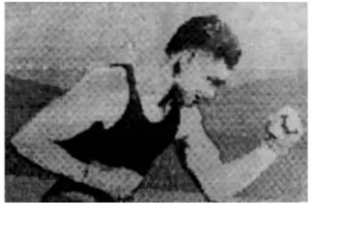
FIGURE 1.2 A digital picture made in 1922 from a tape punched after the signals had crossed the Atlantic twice. (McFarlane.) FIGURE 1.3 Unretouched cable picture of Generals Pershing and Foch, transmitted in 1929 from London to New York by 15-tone equipment. (McFarlane.)
The early Bartlane systems were capable of coding images in five distinct levels of gray. This capability was increased to 15 levels in 1929. Figure 1.3 is typical of the type of images that could be obtained using the 15-tone equip-ment. During this period, introduction of a system for developing a film plate via light beams that were modulated by the coded picture tape improved the reproduction process considerably.
Although the examples just cited involve digital images, they are not con-sidered digital image processing results in the context of our definition be-cause computers were not involved in their creation. Thus, the history of digital image processing is intimately tied to the development of the digital computer. In fact, digital images require so much storage and computational power that progress in the field of digital image processing has been depen-dent on the development of digital computers and of supporting technologies that include data storage, display, and transmission.
The idea of a computer goes back to the invention of the abacus in Asia Minor, more than 5000 years ago. More recently, there were developments in the past two centuries that are the foundation of what we call a computer today. However, the basis for what we call a moderndigital computer dates back to only the 1940s with the introduction by John von Neumann of two key con-cepts: (1) a memory to hold a stored program and data, and (2) conditional branching. These two ideas are the foundation of a central processing unit (CPU), which is at the heart of computers today. Starting with von Neumann, there were a series of key advances that led to computers powerful enough to
be used for digital image processing. Briefly, these advances may be summa-rized as follows: (1) the invention of the transistor at Bell Laboratories in 1948; (2) the development in the 1950s and 1960s of the high-level programming lan-guages COBOL (Common Business-Oriented Language) and FORTRAN (Formula Translator); (3) the invention of the integrated circuit (IC) at Texas Instruments in 1958; (4) the development of operating systems in the early 1960s; (5) the development of the microprocessor (a single chip consisting of the central processing unit, memory, and input and output controls) by Intel in the early 1970s; (6) introduction by IBM of the personal computer in 1981; and (7) progressive miniaturization of components, starting with large scale integra-tion (LI) in the late 1970s, then very large scale integraintegra-tion (VLSI) in the 1980s, to the present use of ultra large scale integration (ULSI). Concurrent with these advances were developments in the areas of mass storage and display sys-tems, both of which are fundamental requirements for digital image processing. The first computers powerful enough to carry out meaningful image pro-cessing tasks appeared in the early 1960s. The birth of what we call digital image processing today can be traced to the availability of those machines and to the onset of the space program during that period. It took the combination of those two developments to bring into focus the potential of digital image processing concepts. Work on using computer techniques for improving im-ages from a space probe began at the Jet Propulsion Laboratory (Pasadena, California) in 1964 when pictures of the moon transmitted by Ranger 7were processed by a computer to correct various types of image distortion inherent in the on-board television camera. Figure 1.4 shows the first image of the moon taken by Ranger 7on July 31, 1964 at 9:09 A.M. Eastern Daylight Time
(EDT), about 17 minutes before impacting the lunar surface (the markers, called reseau marks, are used for geometric corrections, as discussed in Chapter 2). This also is the first image of the moon taken by a U.S. spacecraft. The imaging lessons learned with Ranger 7served as the basis for improved methods used to enhance and restore images from the Surveyor missions to the moon, the Mariner series of flyby missions to Mars, the Apollo manned flights to the moon, and others.
FIGURE 1.4 The first picture of the moon by a U.S. spacecraft.Ranger 7took this image on July 31, 1964 at 9:09 A.M. EDT,
about 17 minutes before impacting the lunar surface. (Courtesy of NASA.)
In parallel with space applications, digital image processing techniques began in the late 1960s and early 1970s to be used in medical imaging, remote Earth resources observations, and astronomy. The invention in the early 1970s of computerized axial tomography (CAT), also called computerized tomogra-phy (CT) for short, is one of the most important events in the application of image processing in medical diagnosis. Computerized axial tomography is a process in which a ring of detectors encircles an object (or patient) and an X-ray source, concentric with the detector ring, rotates about the object. The X-rays pass through the object and are collected at the opposite end by the corresponding detectors in the ring. As the source rotates, this procedure is re-peated. Tomography consists of algorithms that use the sensed data to con-struct an image that represents a “slice” through the object. Motion of the object in a direction perpendicular to the ring of detectors produces a set of such slices, which constitute a three-dimensional (3-D) rendition of the inside of the object. Tomography was invented independently by Sir Godfrey N. Hounsfield and Professor Allan M. Cormack, who shared the 1979 Nobel Prize in Medicine for their invention. It is interesting to note that X-rays were discovered in 1895 by Wilhelm Conrad Roentgen, for which he received the 1901 Nobel Prize for Physics. These two inventions, nearly 100 years apart, led to some of the most important applications of image processing today.
From the 1960s until the present, the field of image processing has grown vigorously. In addition to applications in medicine and the space program, dig-ital image processing techniques now are used in a broad range of applica-tions. Computer procedures are used to enhance the contrast or code the intensity levels into color for easier interpretation of X-rays and other images used in industry, medicine, and the biological sciences. Geographers use the same or similar techniques to study pollution patterns from aerial and satellite imagery. Image enhancement and restoration procedures are used to process degraded images of unrecoverable objects or experimental results too expen-sive to duplicate. In archeology, image processing methods have successfully restored blurred pictures that were the only available records of rare artifacts lost or damaged after being photographed. In physics and related fields, com-puter techniques routinely enhance images of experiments in areas such as high-energy plasmas and electron microscopy. Similarly successful applica-tions of image processing concepts can be found in astronomy, biology, nuclear medicine, law enforcement, defense, and industry.
These examples illustrate processing results intended for human interpreta-tion. The second major area of application of digital image processing tech-niques mentioned at the beginning of this chapter is in solving problems dealing with machine perception. In this case, interest is on procedures for extracting from an image information in a form suitable for computer processing. Often, this information bears little resemblance to visual features that humans use in interpreting the content of an image. Examples of the type of information used in machine perception are statistical moments, Fourier transform coefficients, and multidimensional distance measures. Typical problems in machine percep-tion that routinely utilize image processing techniques are automatic character recognition, industrial machine vision for product assembly and inspection,
military recognizance, automatic processing of fingerprints, screening of X-rays and blood samples, and machine processing of aerial and satellite imagery for weather prediction and environmental assessment.The continuing decline in the ratio of computer price to performance and the expansion of networking and communication bandwidth via the World Wide Web and the Internet have cre-ated unprecedented opportunities for continued growth of digital image pro-cessing. Some of these application areas are illustrated in the following section.
1.3
Examples of Fields that Use Digital Image Processing
Today, there is almost no area of technical endeavor that is not impacted in some way by digital image processing. We can cover only a few of these appli-cations in the context and space of the current discussion. However, limited as it is, the material presented in this section will leave no doubt in your mind re-garding the breadth and importance of digital image processing. We show in this section numerous areas of application, each of which routinely utilizes the digital image processing techniques developed in the following chapters. Many of the images shown in this section are used later in one or more of the exam-ples given in the book. All images shown are digital.The areas of application of digital image processing are so varied that some form of organization is desirable in attempting to capture the breadth of this field. One of the simplest ways to develop a basic understanding of the extent of image processing applications is to categorize images according to their source (e.g., visual, X-ray, and so on).The principal energy source for images in use today is the electromagnetic energy spectrum. Other important sources of energy in-clude acoustic, ultrasonic, and electronic (in the form of electron beams used in electron microscopy). Synthetic images, used for modeling and visualization, are generated by computer. In this section we discuss briefly how images are gener-ated in these various categories and the areas in which they are applied. Methods for converting images into digital form are discussed in the next chapter.
Images based on radiation from the EM spectrum are the most familiar, especially images in the X-ray and visual bands of the spectrum. Electromag-netic waves can be conceptualized as propagating sinusoidal waves of varying wavelengths, or they can be thought of as a stream of massless particles, each traveling in a wavelike pattern and moving at the speed of light. Each mass-less particle contains a certain amount (or bundle) of energy. Each bundle of energy is called a photon. If spectral bands are grouped according to energy per photon, we obtain the spectrum shown in Fig. 1.5, ranging from gamma rays (highest energy) at one end to radio waves (lowest energy) at the other.
10⫺9 10⫺8 10⫺7 10⫺6 10⫺5 10⫺4 10⫺3 10⫺2 100 10⫺1 101 102 103 104 105 106
Energy of one photon (electron volts)
Gamma rays X-rays Ultraviolet Visible Infrared Microwaves Radio waves
The bands are shown shaded to convey the fact that bands of the EM spec-trum are not distinct but rather transition smoothly from one to the other.
1.3.1 Gamma-Ray Imaging
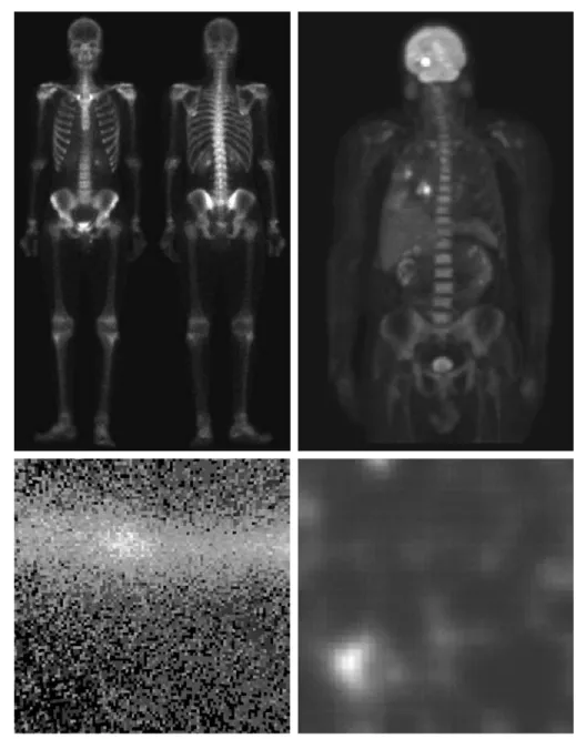
Major uses of imaging based on gamma rays include nuclear medicine and as-tronomical observations. In nuclear medicine, the approach is to inject a pa-tient with a radioactive isotope that emits gamma rays as it decays. Images are produced from the emissions collected by gamma ray detectors. Figure 1.6(a) shows an image of a complete bone scan obtained by using gamma-ray imaging. Images of this sort are used to locate sites of bone pathology, such as infections
FIGURE 1.6 Examples of gamma-ray imaging. (a) Bone scan. (b) PET image. (c) Cygnus Loop. (d) Gamma radiation (bright spot) from a reactor valve. (Images courtesy of (a) G.E. Medical Systems, (b) Dr. Michael E. Casey, CTI PET Systems, (c) NASA, (d) Professors Zhong He and David K. Wehe, University of Michigan.) a b c d
or tumors. Figure 1.6(b) shows another major modality of nuclear imaging called positron emission tomography (PET). The principle is the same as with X-ray tomography, mentioned briefly in Section 1.2. However, instead of using an external source of X-ray energy, the patient is given a radioactive isotope that emits positrons as it decays. When a positron meets an electron, both are annihilated and two gamma rays are given off. These are detected and a tomo-graphic image is created using the basic principles of tomography. The image shown in Fig. 1.6(b) is one sample of a sequence that constitutes a 3-D rendition of the patient. This image shows a tumor in the brain and one in the lung, easily visible as small white masses.
A star in the constellation of Cygnus exploded about 15,000 years ago, gener-ating a superheated stationary gas cloud (known as the Cygnus Loop) that glows in a spectacular array of colors. Figure 1.6(c) shows an image of the Cygnus Loop in the gamma-ray band. Unlike the two examples in Figs. 1.6(a) and (b), this image was obtained using the natural radiation of the object being imaged. Finally, Fig. 1.6(d) shows an image of gamma radiation from a valve in a nuclear reactor. An area of strong radiation is seen in the lower left side of the image.
1.3.2 X-Ray Imaging
X-rays are among the oldest sources of EM radiation used for imaging. The best known use of X-rays is medical diagnostics, but they also are used exten-sively in industry and other areas, like astronomy. X-rays for medical and in-dustrial imaging are generated using an X-ray tube, which is a vacuum tube with a cathode and anode. The cathode is heated, causing free electrons to be released. These electrons flow at high speed to the positively charged anode. When the electrons strike a nucleus, energy is released in the form of X-ray radiation. The energy (penetrating power) of X-rays is controlled by a voltage applied across the anode, and by a current applied to the filament in the cathode. Figure 1.7(a) shows a familiar chest X-ray generated simply by plac-ing the patient between an X-ray source and a film sensitive to X-ray energy. The intensity of the X-rays is modified by absorption as they pass through the patient, and the resulting energy falling on the film develops it, much in the same way that light develops photographic film. In digital radiography, digital images are obtained by one of two methods: (1) by digitizing X-ray films; or (2) by having the X-rays that pass through the patient fall directly onto devices (such as a phosphor screen) that convert X-rays to light. The light signal in turn is captured by a light-sensitive digitizing system. We discuss digitization in more detail in Chapters 2 and 4.
Angiography is another major application in an area called contrast-enhancement radiography. This procedure is used to obtain images (called angiograms) of blood vessels. A catheter (a small, flexible, hollow tube) is in-serted, for example, into an artery or vein in the groin. The catheter is threaded into the blood vessel and guided to the area to be studied. When the catheter reaches the site under investigation, an X-ray contrast medium is injected through the tube. This enhances contrast of the blood vessels and enables the radiologist to see any irregularities or blockages. Figure 1.7(b) shows an exam-ple of an aortic angiogram. The catheter can be seen being inserted into the
FIGURE 1.7 Examples of X-ray imaging. (a) Chest X-ray. (b) Aortic angiogram. (c) Head CT. (d) Circuit boards. (e) Cygnus Loop. (Images courtesy of (a) and (c) Dr. David R. Pickens, Dept. of Radiology & Radiological Sciences, Vanderbilt University Medical Center; (b) Dr. Thomas R. Gest, Division of Anatomical Sciences, University of Michigan Medical School; (d) Mr. Joseph E. Pascente, Lixi, Inc.; and (e) NASA.)
a b c
d e
large blood vessel on the lower left of the picture. Note the high contrast of the large vessel as the contrast medium flows up in the direction of the kidneys, which are also visible in the image. As discussed in Chapter 2, angiography is a major area of digital image processing, where image subtraction is used to en-hance further the blood vessels being studied.
Another important use of X-rays in medical imaging is computerized axial to-mography (CAT). Due to their resolution and 3-D capabilities, CAT scans revo-lutionized medicine from the moment they first became available in the early 1970s. As noted in Section 1.2, each CAT image is a “slice” taken perpendicularly through the patient. Numerous slices are generated as the patient is moved in a longitudinal direction.The ensemble of such images constitutes a 3-D rendition of the inside of the body, with the longitudinal resolution being proportional to the number of slice images taken. Figure 1.7(c) shows a typical head CAT slice image. Techniques similar to the ones just discussed, but generally involving higher-energy X-rays, are applicable in industrial processes. Figure 1.7(d) shows an X-ray image of an electronic circuit board. Such images, representative of literally hun-dreds of industrial applications of X-rays, are used to examine circuit boards for flaws in manufacturing, such as missing components or broken traces. Industrial CAT scans are useful when the parts can be penetrated by X-rays, such as in plastic assemblies, and even large bodies, like solid-propellant rocket motors. Figure 1.7(e) shows an example of X-ray imaging in astronomy.This image is the Cygnus Loop of Fig. 1.6(c), but imaged this time in the X-ray band.
1.3.3 Imaging in the Ultraviolet Band
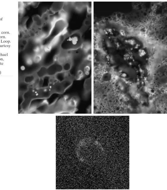
Applications of ultraviolet “light” are varied. They include lithography, industrial inspection, microscopy, lasers, biological imaging, and astronomical observations. We illustrate imaging in this band with examples from microscopy and astronomy. Ultraviolet light is used in fluorescence microscopy, one of the fastest grow-ing areas of microscopy. Fluorescence is a phenomenon discovered in the mid-dle of the nineteenth century, when it was first observed that the mineral fluorspar fluoresces when ultraviolet light is directed upon it. The ultraviolet light itself is not visible, but when a photon of ultraviolet radiation collides with an electron in an atom of a fluorescent material, it elevates the electron to a higher energy level. Subsequently, the excited electron relaxes to a lower level and emits light in the form of a lower-energy photon in the visible (red) light region. The basic task of the fluorescence microscope is to use an excitation light to irradiate a prepared specimen and then to separate the much weaker radiating fluores-cent light from the brighter excitation light. Thus, only the emission light reaches the eye or other detector. The resulting fluorescing areas shine against a dark background with sufficient contrast to permit detection. The darker the back-ground of the nonfluorescing material, the more efficient the instrument.
Fluorescence microscopy is an excellent method for studying materials that can be made to fluoresce, either in their natural form (primary fluorescence) or when treated with chemicals capable of fluorescing (secondary fluorescence). Figures 1.8(a) and (b) show results typical of the capability of fluorescence microscopy. Figure 1.8(a) shows a fluorescence microscope image of normal corn, and Fig. 1.8(b) shows corn infected by “smut,” a disease of cereals, corn,
grasses, onions, and sorghum that can be caused by any of more than 700 species of parasitic fungi. Corn smut is particularly harmful because corn is one of the principal food sources in the world. As another illustration, Fig. 1.8(c) shows the Cygnus Loop imaged in the high-energy region of the ultraviolet band.
1.3.4 Imaging in the Visible and Infrared Bands
Considering that the visual band of the electromagnetic spectrum is the most familiar in all our activities, it is not surprising that imaging in this band out-weighs by far all the others in terms of breadth of application. The infrared band often is used in conjunction with visual imaging, so we have grouped the FIGURE 1.8
Examples of ultraviolet imaging. (a) Normal corn. (b) Smut corn. (c) Cygnus Loop. (Images courtesy of (a) and (b) Dr. Michael W. Davidson, Florida State University, (c) NASA.) a c b
visible and infrared bands in this section for the purpose of illustration. We consider in the following discussion applications in light microscopy, astrono-my, remote sensing, industry, and law enforcement.
Figure 1.9 shows several examples of images obtained with a light microscope. The examples range from pharmaceuticals and microinspection to materials characterization. Even in microscopy alone, the application areas are too numer-ous to detail here. It is not difficult to conceptualize the types of processes one might apply to these images, ranging from enhancement to measurements.
FIGURE 1.9 Examples of light microscopy images. (a) Taxol (anticancer agent), magnified (b) Cholesterol— (c) Microprocessor— (d) Nickel oxide thin film— (e) Surface of audio CD— (f) Organic superconductor—
(Images courtesy of Dr. Michael W. Davidson, Florida State University.) 450*. 1750*. 600*. 60*. 40*. 250*. a b c d e f
Another major area of visual processing is remote sensing, which usually in-cludes several bands in the visual and infrared regions of the spectrum. Table 1.1 shows the so-called thematic bandsin NASA’s LANDSAT satellite. The primary function of LANDSAT is to obtain and transmit images of the Earth from space for purposes of monitoring environmental conditions on the planet. The bands are expressed in terms of wavelength, with m being equal to (we dis-cuss the wavelength regions of the electromagnetic spectrum in more detail in Chapter 2). Note the characteristics and uses of each band in Table 1.1.
In order to develop a basic appreciation for the power of this type of multispectral imaging, consider Fig. 1.10, which shows one image for each of
10-6
m 1
1 2 3
4 5 6 7
FIGURE 1.10 LANDSAT satellite images of the Washington, D.C. area. The numbers refer to the thematic bands in Table 1.1. (Images courtesy of NASA.)
Band No. Name Wavelength (m) Characteristics and Uses
1 Visible blue 0.45–0.52 Maximum water
penetration
2 Visible green 0.52–0.60 Good for measuring plant
vigor
3 Visible red 0.63–0.69 Vegetation discrimination
4 Near infrared 0.76–0.90 Biomass and shoreline
mapping
5 Middle infrared 1.55–1.75 Moisture content of soil and vegetation 6 Thermal infrared 10.4–12.5 Soil moisture; thermal
mapping
7 Middle infrared 2.08–2.35 Mineral mapping
TABLE 1.1 Thematic bands in NASA’s LANDSAT satellite.
the spectral bands in Table 1.1. The area imaged is Washington D.C., which in-cludes features such as buildings, roads, vegetation, and a major river (the Po-tomac) going though the city. Images of population centers are used routinely (over time) to assess population growth and shift patterns, pollution, and other factors harmful to the environment. The differences between visual and in-frared image features are quite noticeable in these images. Observe, for exam-ple, how well defined the river is from its surroundings in Bands 4 and 5.
Weather observation and prediction also are major applications of multi-spectral imaging from satellites. For example, Fig. 1.11 is an image of Hurricane Katrina one of the most devastating storms in recent memory in the Western Hemisphere. This image was taken by a National Oceanographic and Atmos-pheric Administration (NOAA) satellite using sensors in the visible and in-frared bands. The eye of the hurricane is clearly visible in this image.
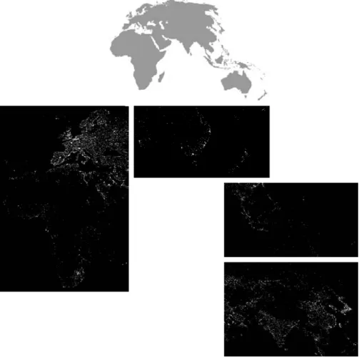
Figures 1.12 and 1.13 show an application of infrared imaging. These images are part of the Nighttime Lights of the Worlddata set, which provides a global inventory of human settlements. The images were generated by the infrared imaging system mounted on a NOAA DMSP (Defense Meteorological Satel-lite Program) satelSatel-lite. The infrared imaging system operates in the band 10.0 to m, and has the unique capability to observe faint sources of visible-near infrared emissions present on the Earth’s surface, including cities, towns, villages, gas flares, and fires. Even without formal training in image processing, it is not difficult to imagine writing a computer program that would use these im-ages to estimate the percent of total electrical energy used by various regions of the world.
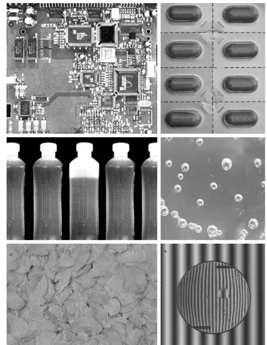
A major area of imaging in the visual spectrum is in automated visual in-spection of manufactured goods. Figure 1.14 shows some examples. Figure 1.14(a) is a controller board for a CD-ROM drive. A typical image processing task with products like this is to inspect them for missing parts (the black square on the top, right quadrant of the image is an example of a missing component).
13.4 FIGURE 1.11 Satellite image of Hurricane Katrina taken on August 29, 2005. (Courtesy of NOAA.)
Figure 1.14(b) is an imaged pill container. The objective here is to have a ma-chine look for missing pills. Figure 1.14(c) shows an application in which image processing is used to look for bottles that are not filled up to an acceptable level. Figure 1.14(d) shows a clear-plastic part with an unacceptable number of air pockets in it. Detecting anomalies like these is a major theme of industrial inspection that includes other products such as wood and cloth. Figure 1.14(e) FIGURE 1.12
Infrared satellite images of the Americas. The small gray map is provided for reference. (Courtesy of NOAA.)
shows a batch of cereal during inspection for color and the presence of anom-alies such as burned flakes. Finally, Fig. 1.14(f) shows an image of an intraocular implant (replacement lens for the human eye). A “structured light” illumina-tion technique was used to highlight for easier detecillumina-tion flat lens deformaillumina-tions toward the center of the lens. The markings at 1 o’clock and 5 o’clock are tweezer damage. Most of the other small speckle detail is debris. The objective in this type of inspection is to find damaged or incorrectly manufactured im-plants automatically, prior to packaging.
As a final illustration of image processing in the visual spectrum, consider Fig. 1.15. Figure 1.15(a) shows a thumb print. Images of fingerprints are rou-tinely processed by computer, either to enhance them or to find features that aid in the automated search of a database for potential matches. Figure 1.15(b) shows an image of paper currency. Applications of digital image processing in this area include automated counting and, in law enforcement, the reading of the serial number for the purpose of tracking and identifying bills. The two ve-hicle images shown in Figs. 1.15 (c) and (d) are examples of automated license plate reading. The light rectangles indicate the area in which the imaging system
FIGURE 1.13 Infrared satellite images of the remaining populated part of the world. The small gray map is provided for reference. (Courtesy of NOAA.)
detected the plate. The black rectangles show the results of automated reading of the plate content by the system. License plate and other applications of char-acter recognition are used extensively for traffic monitoring and surveillance.
1.3.5 Imaging in the Microwave Band
The dominant application of imaging in the microwave band is radar. The unique feature of imaging radar is its ability to collect data over virtually any region at any time, regardless of weather or ambient lighting conditions. Some FIGURE 1.14 Some examples of manufactured goods often checked using digital image processing. (a) A circuit board controller. (b) Packaged pills. (c) Bottles. (d) Air bubbles in a clear-plastic product. (e) Cereal. (f) Image of intraocular implant. (Fig. (f) courtesy of Mr. Pete Sites, Perceptics Corporation.) a c e b d f
radar waves can penetrate clouds, and under certain conditions can also see through vegetation, ice, and dry sand. In many cases, radar is the only way to explore inaccessible regions of the Earth’s surface. An imaging radar works like a flash camera in that it provides its own illumination (microwave pulses) to illuminate an area on the ground and take a snapshot image. Instead of a camera lens, a radar uses an antenna and digital computer processing to record its images. In a radar image, one can see only the microwave energy that was reflected back toward the radar antenna.
Figure 1.16 shows a spaceborne radar image covering a rugged mountain-ous area of southeast Tibet, about 90 km east of the city of Lhasa. In the lower right corner is a wide valley of the Lhasa River, which is populated by Tibetan farmers and yak herders and includes the village of Menba. Mountains in this area reach about 5800 m (19,000 ft) above sea level, while the valley floors lie about 4300 m (14,000 ft) above sea level. Note the clarity and detail of the image, unencumbered by clouds or other atmospheric conditions that normally interfere with images in the visual band.
FIGURE 1.15 Some additional examples of imaging in the visual spectrum. (a) Thumb print. (b) Paper currency. (c) and (d) Automated license plate reading. (Figure (a) courtesy of the National Institute of Standards and Technology. Figures (c) and (d) courtesy of Dr. Juan Herrera, Perceptics Corporation.) a b c d
FIGURE 1.16 Spaceborne radar image of mountains in southeast Tibet. (Courtesy of NASA.)
1.3.6 Imaging in the Radio Band
As in the case of imaging at the other end of the spectrum (gamma rays), the major applications of imaging in the radio band are in medicine and astronomy. In medicine, radio waves are used in magnetic resonance imaging (MRI). This technique places a patient in a powerful magnet and passes radio waves through his or her body in short pulses. Each pulse causes a responding pulse of radio waves to be emitted by the patient’s tissues. The location from which these sig-nals originate and their strength are determined by a computer, which produces a two-dimensional picture of a section of the patient. MRI can produce pictures in any plane. Figure 1.17 shows MRI images of a human knee and spine.
The last image to the right in Fig. 1.18 shows an image of the Crab Pulsar in the radio band. Also shown for an interesting comparison are images of the same region but taken in most of the bands discussed earlier. Note that each image gives a totally different “view” of the Pulsar.
1.3.7 Examples in which Other Imaging Modalities Are Used
Although imaging in the electromagnetic spectrum is dominant by far, there are a number of other imaging modalities that also are important. Specifically, we discuss in this section acoustic imaging, electron microscopy, and synthetic (computer-generated) imaging.
Imaging using “sound” finds application in geological exploration, industry, and medicine. Geological applications use sound in the low end of the sound spectrum (hundreds of Hz) while imaging in other areas use ultrasound (mil-lions of Hz). The most important commercial applications of image processing in geology are in mineral and oil exploration. For image acquisition over land, one of the main approaches is to use a large truck and a large flat steel plate. The plate is pressed on the ground by the truck, and the truck is vibrated through a frequency spectrum up to 100 Hz. The strength and speed of the
FIGURE 1.17 MRI images of a human (a) knee, and (b) spine. (Image (a) courtesy of Dr. Thomas R. Gest, Division of Anatomical Sciences, University of Michigan Medical School, and (b) courtesy of Dr. David R. Pickens, Department of Radiology and Radiological Sciences, Vanderbilt University Medical Center.)
Gamma X-ray Optical Infrared Radio
FIGURE 1.18 Images of the Crab Pulsar (in the center of each image) covering the electromagnetic spectrum. (Courtesy of NASA.)
returning sound waves are determined by the composition of the Earth below the surface. These are analyzed by computer, and images are generated from the resulting analysis.
For marine acquisition, the energy source consists usually of two air guns towed behind a ship. Returning sound waves are detected by hydrophones placed in cables that are either towed behind the ship, laid on the bottom of the ocean, or hung from buoys (vertical cables). The two air guns are alter-nately pressurized to and then set off. The constant motion of the ship provides a transversal direction of motion that, together with the return-ing sound waves, is used to generate a 3-D map of the composition of the Earth below the bottom of the ocean.
Figure 1.19 shows a cross-sectional image of a well-known 3-D model against which the performance of seismic imaging algorithms is tested. The arrow points to a hydrocarbon (oil and/or gas) trap. This target is brighter than the surrounding layers because the change in density in the target region is
'2000 psi
larger. Seismic interpreters look for these “bright spots” to find oil and gas. The layers above also are bright, but their brightness does not vary as strongly across the layers. Many seismic reconstruction algorithms have difficulty imag-ing this target because of the faults above it.
Although ultrasound imaging is used routinely in manufacturing, the best known applications of this technique are in medicine, especially in obstetrics, where unborn babies are imaged to determine the health of their develop-ment. A byproduct of this examination is determining the sex of the baby. Ul-trasound images are generated using the following basic procedure:
1. The ultrasound system (a computer, ultrasound probe consisting of a source and receiver, and a display) transmits high-frequency (1 to 5 MHz) sound pulses into the body.
2. The sound waves travel into the body and hit a boundary between tissues (e.g., between fluid and soft tissue, soft tissue and bone). Some of the sound waves are reflected back to the probe, while some travel on further until they reach another boundary and get reflected.
3. The reflected waves are picked up by the probe and relayed to the com-puter.
4. The machine calculates the distance from the probe to the tissue or organ boundaries using the speed of sound in tissue (1540 m/s) and the time of each echo’s return.
5. The system displays the distances and intensities of the echoes on the screen, forming a two-dimensional image.
In a typical ultrasound image, millions of pulses and echoes are sent and re-ceived each second. The probe can be moved along the surface of the body and angled to obtain various views. Figure 1.20 shows several examples.
We continue the discussion on imaging modalities with some examples of electron microscopy. Electron microscopes function as their optical counter-parts, except that they use a focused beam of electrons instead of light to image a specimen. The operation of electron microscopes involves the follow-ing basic steps: A stream of electrons is produced by an electron source and ac-celerated toward the specimen using a positive electrical potential. This stream FIGURE 1.19
Cross-sectional image of a seismic model. The arrow points to a hydrocarbon (oil and/or gas) trap. (Courtesy of Dr. Curtis Ober, Sandia National Laboratories.)
is confined and focused using metal apertures and magnetic lenses into a thin, monochromatic beam. This beam is focused onto the sample using a magnetic lens. Interactions occur inside the irradiated sample, affecting the electron beam. These interactions and effects are detected and transformed into an image, much in the same way that light is reflected from, or absorbed by, ob-jects in a scene. These basic steps are carried out in all electron microscopes. A transmission electron microscope(TEM) works much like a slide projec-tor. A projector shines (transmits) a beam of light through a slide; as the light passes through the slide, it is modulated by the contents of the slide. This trans-mitted beam is then projected onto the viewing screen, forming an enlarged image of the slide. TEMs work the same way, except that they shine a beam of electrons through a specimen (analogous to the slide). The fraction of the beam transmitted through the specimen is projected onto a phosphor screen. The interaction of the electrons with the phosphor produces light and, there-fore, a viewable image. A scanning electron microscope(SEM), on the other hand, actually scans the electron beam and records the interaction of beam and sample at each location. This produces one dot on a phosphor screen. A complete image is formed by a raster scan of the beam through the sample, much like a TV camera. The electrons interact with a phosphor screen and produce light. SEMs are suitable for “bulky” samples, while TEMs require very thin samples.
Electron microscopes are capable of very high magnification. While light microscopy is limited to magnifications on the order 1000*,electron microscopes
FIGURE 1.20 Examples of ultrasound imaging. (a) Baby. (b) Another view of baby. (c) Thyroids. (d) Muscle layers showing lesion. (Courtesy of Siemens Medical Systems, Inc., Ultrasound Group.) a b c d
can achieve magnification of or more. Figure 1.21 shows two SEM im-ages of specimen failures due to thermal overload.
We conclude the discussion of imaging modalities by looking briefly at im-ages that are not obtained from physical objects. Instead, they are generated by computer. Fractals are striking examples of computer-generated images (Lu [1997]). Basically, a fractal is nothing more than an iterative reproduction of a basic pattern according to some mathematical rules. For instance,tilingis one of the simplest ways to generate a fractal image. A square can be subdi-vided into four square subregions, each of which can be further subdisubdi-vided into four smaller square regions, and so on. Depending on the complexity of the rules for filling each subsquare, some beautiful tile images can be generated using this method. Of course, the geometry can be arbitrary. For instance, the fractal image could be grown radially out of a center point. Figure 1.22(a) shows a fractal grown in this way. Figure 1.22(b) shows another fractal (a “moonscape”) that provides an interesting analogy to the images of space used as illustrations in some of the preceding sections.
Fractal images tend toward artistic, mathematical formulations of “growth” of subimage elements according to a set of rules. They are useful sometimes as random textures. A more structured approach to image generation by computer lies in 3-D modeling. This is an area that provides an important intersection between image processing and computer graphics and is the basis for many 3-D visualization systems (e.g., flight simulators). Figures 1.22(c) and (d) show examples of computer-generated images. Since the original object is created in 3-D, images can be generated in any perspective from plane projections of the 3-D volume. Images of this type can be used for medical training and for a host of other applications, such as criminal forensics and special effects.
10,000*
FIGURE 1.21 (a) SEM image of a tungsten filament following thermal failure (note the shattered pieces on the lower left). (b) SEM image of damaged integrated circuit. The white fibers are oxides resulting from thermal destruction. (Figure (a) courtesy of Mr. Michael Shaffer, Department of Geological Sciences, University of Oregon, Eugene; (b) courtesy of Dr. J. M. Hudak, McMaster University, Hamilton, Ontario, Canada.)
2500* 250*
1.4
Fundamental Steps in Digital Image Processing
It is helpful to divide the material covered in the following chapters into the two broad categories defined in Section 1.1: methods whose input and output are images, and methods whose inputs may be images but whose outputs are attributes extracted from those images. This organization is summarized in Fig. 1.23. The diagram does not imply that every process is applied to an image. Rather, the intention is to convey an idea of all the methodologies that can be applied to images for different purposes and possibly with different objectives. The discussion in this section may be viewed as a brief overview of the material in the remainder of the book.
Image acquisitionis the first process in Fig. 1.23. The discussion in Section 1.3 gave some hints regarding the origin of digital images. This topic is considered in much more detail in Chapter 2, where we also introduce a number of basic digital image concepts that are used throughout the book. Note that acquisi-tion could be as simple as being given an image that is already in digital form. Generally, the image acquisition stage involves preprocessing, such as scaling. Image enhancementis the process of manipulating an image so that the re-sult is more suitable than the original for a specific application. The word specificis important here, because it establishes at the outset that enhancement techniques are problem oriented. Thus, for example, a method that is quite use-ful for enhancing X-ray images may not be the best approach for enhancing satellite images taken in the infrared band of the electromagnetic spectrum.
FIGURE 1.22 (a) and (b) Fractal images. (c) and (d) Images generated from 3-D computer models of the objects shown. (Figures (a) and (b) courtesy of Ms. Melissa D. Binde, Swarthmore College; (c) and (d) courtesy of NASA.) a b c d
Knowledge base CHAPTER 7 Wavelets and multiresolution processing CHAPTER 6 Color image processing
Outputs of these processes generally are images
CHAPTER 5 Image restoration CHAPTERS 3 & 4 Image filtering and enhancement Problem domain
Outputs of these processes generally are image attributes
CHAPTER 8 Compression CHAPTER 2 Image acquisition CHAPTER 9 Morphological processing CHAPTER 10 Segmentation CHAPTER 11 Representation & description CHAPTER 12 Object recognition FIGURE 1.23 Fundamental steps in digital image processing. The chapter(s) indicated in the boxes is where the material
described in the box is discussed.
There is no general “theory” of image enhancement. When an image is processed for visual interpretation, the viewer is the ultimate judge of how well a particular method works. Enhancement techniques are so varied, and use so many different image processing approaches, that it is difficult to as-semble a meaningful body of techniques suitable for enhancement in one chapter without extensive background development. For this reason, and also because beginners in the field of image processing generally find enhance-ment applications visually appealing, interesting, and relatively simple to un-derstand, we use image enhancement as examples when introducing new concepts in parts of Chapter 2 and in Chapters 3 and 4. The material in the latter two chapters span many of the methods used traditionally for image en-hancement. Therefore, using examples from image enhancement to introduce new image processing methods developed in these early chapters not only saves having an extra chapter in the book dealing with image enhancement but, more importantly, is an effective approach for introducing newcomers to the details of processing techniques early in the book. However, as you will see in progressing through the rest of the book, the material developed in these chapters is applicable to a much broader class of problems than just image enhancement.
Image restorationis an area that also deals with improving the appearance of an image. However, unlike enhancement, which is subjective, image restora-tion is objective, in the sense that restorarestora-tion techniques tend to be based on mathematical or probabilistic models of image degradation. Enhancement, on the other hand, is based on human subjective preferences regarding what con-stitutes a “good” enhancement result.
Color image processingis an area that has been gaining in importance be-cause of the significant increase in the use of digital images over the Internet. Chapter 6 covers a number of fundamental concepts in color models and basic color processing in a digital domain. Color is used also in later chapters as the basis for extracting features of interest in an image.
Waveletsare the foundation for representing images in various degrees of resolution. In particular, this material is used in this book for image data com-pression and for pyramidal representation, in which images are subdivided successively into smaller regions.
Compression, as the name implies, deals with techniques for reducing the storage required to save an image, or the bandwidth required to transmit it. Al-though storage technology has improved significantly over the past decade, the same cannot be said for transmission capacity. This is true particularly in uses of the Internet, which are characterized by significant pictorial content. Image compression is familiar (perhaps inadvertently) to most users of computers in the form of image file extensions, such as the jpg file extension used in the JPEG (Joint Photographic Experts Group) image compression standard.
Morphological processingdeals with tools for extracting image components that are useful in the representation and description of shape. The material in this chapter begins a transition from processes that output images to processes that output image attributes, as indicated in Section 1.1.
Segmentation procedures partition an image into its constituent parts or objects. In general, autonomous segmentation is one of the most difficult tasks in digital image processing. A rugged segmentation procedure brings the process a long way toward successful solution of imaging problems that require objects to be identified individually. On the other hand, weak or er-ratic segmentation algorithms almost always guarantee eventual failure. In general, the more accurate the segmentation, the more likely recognition is to succeed.
Representation and descriptionalmost always follow the output of a segmen-tation stage, which usually is raw pixel data, constituting either the boundary of a region (i.e., the set of pixels separating one image region from another) or all the points in the region itself. In either case, converting the data to a form suit-able for computer processing is necessary. The first decision that must be made is whether the data should be represented as a boundary or as a complete region. Boundary representation is appropriate when the focus is on external shape characteristics, such as corners and inflections. Regional representation is ap-propriate when the focus is on internal properties, such as texture or skeletal shape. In some applications, these representations complement each other. Choosing a representation is only part of the solution for transforming raw data into a form suitable for subsequent computer processing. A method must also be specified for describing the data so that features of interest are high-lighted.Description, also called feature selection, deals with extracting attributes that result in some quantitative information of interest or are basic for differ-entiating one class of objects from another.
Recognitionis the process that assigns a label (e.g., “vehicle”) to an object based on its descriptors. As detailed in Section 1.1, we conclude our coverage of
digital image processing with the development of methods for recognition of individual objects.
So far we have said nothing about the need for prior knowledge or about the interaction between the knowledge baseand the processing modules in Fig. 1.23. Knowledge about a problem domain is coded into an image processing system in the form of a knowledge database. This knowledge may be as simple as de-tailing regions of an image where the information of interest is known to be located, thus limiting the search that has to be conducted in seeking that infor-mation. The knowledge base also can be quite complex, such as an interrelated list of all major possible defects in a materials inspection problem or an image database containing high-resolution satellite images of a region in connection with change-detection applications. In addition to guiding the operation of each processing module, the knowledge base also controls the interaction between modules.This distinction is made in Fig. 1.23 by the use of double-headed arrows between the processing modules and the knowledge base, as opposed to single-headed arrows linking the processing modules.
Although we do not discuss image display explicitly at this point, it is impor-tant to keep in mind that viewing the results of image processing can take place at the output of any stage in Fig. 1.23. We also note that not all image process-ing applications require the complexity of interactions implied by Fig. 1.23. In fact, not even all those modules are needed in many cases. For example, image enhancement for human visual interpretation seldom requires use of any of the other stages in Fig. 1.23. In general, however, as the complexity of an image pro-cessing task increases, so does the number of processes required to solve the problem.
1.5
Components of an Image Processing System
As recently as the mid-1980s, numerous models of image processing systems being sold throughout the world were rather substantial peripheral devices that attached to equally substantial host computers. Late in the 1980s and early in the 1990s, the market shifted to image processing hardware in the form of single boards designed to be compatible with industry standard buses and to fit into engineering workstation cabinets and personal computers. In addition to lowering costs, this market shift also served as a catalyst for a sig-nificant number of new companies specializing in the development of software written specifically for image processing.
Although large-scale image processing systems still are being sold for mas-sive imaging applications, such as processing of satellite images, the trend con-tinues toward miniaturizing and blending of general-purpose small computers with specialized image processing hardware. Figure 1.24 shows the basic com-ponents comprising a typical general-purpose system used for digital image processing. The function of each component is discussed in the following para-graphs, starting with image sensing.
With reference to sensing, two elements are required to acquire digital im-ages. The first is a physical device that is sensitive to the energy radiated by the object we wish to image. The second, called a digitizer, is a device for converting
the output of the physical sensing device into digital form. For instance, in a digital video camera, the sensors produce an electrical output proportional to light intensity. The digitizer converts these outputs to digital data. These topics are covered in Chapter 2.
Specialized image processing hardwareusually consists of the digitizer just mentioned, plus hardware that performs other primitive operations, such as an arithmetic logic unit (ALU), that performs arithmetic and logical operations in parallel on entire images. One example of how an ALU is used is in averag-ing images as quickly as they are digitized, for the purpose of noise reduction. This type of hardware sometimes is called a front-end subsystem, and its most distinguishing characteristic is speed. In other words, this unit performs func-tions that require fast data throughputs (e.g., digitizing and averaging video images at 30 frames/s) that the typical main computer cannot handle.
The computerin an image processing system is a general-purpose computer and can range from a PC to a supercomputer. In dedicated applications, some-times custom computers are used to achieve a required level of performance, but our interest here is on general-purpose image processing systems. In these systems, almost any well-equipped PC-type machine is suitable for off-line image processing tasks.
Softwarefor image processing consists of specialized modules that perform specific tasks. A well-designed package also includes the capability for the user
Image displays Computer Mass storage
Hardcopy Specialized image processing hardware Image sensors Problem domain Image processing software Network FIGURE 1.24 Components of a general-purpose image processing system.
to write code that, as a minimum, utilizes the specialized modules. More so-phisticated software packages allow the integration of those modules and general-purpose software commands from at least one computer language.
Mass storage capability is a must in image processing applications. An image of size pixels, in which the intensity of each pixel is an 8-bit quantity, requires one megabyte of storage space if the image is not com-pressed. When dealing with thousands, or even millions, of images, providing adequate storage in an image processing system can be a challenge. Digital storage for image processing applications falls into three principal categories: (1) short-term storage for use during processing, (2) on-line storage for rela-tively fast recall, and (3) archival storage, characterized by infrequent access. Storage is measured in bytes (eight bits), Kbytes (one thousand bytes), Mbytes (one million bytes), Gbytes (meaning giga, or one billion, bytes), and Tbytes (meaning tera, or one trillion, bytes).
One method of providing short-term storage is computer memory. An-other is by specialized boards, called frame buffers, that store one or more images and can be accessed rapidly, usually at video rates (e.g., at 30 com-plete images per second). The latter method allows virtually instantaneous image zoom, as well as scroll (vertical shifts) and pan (horizontal shifts). Frame buffers usually are housed in the specialized image processing hard-ware unit in Fig. 1.24. On-line storage generally takes the form of magnetic disks or optical-media storage. The key factor characterizing on-line storage is frequent access to the stored data. Finally, archival storage is characterized by massive storage requirements but infrequent need for access. Magnetic tapes and optical disks housed in “jukeboxes” are the usual media for archival applications.
Image displays in use today are mainly color (preferably flat screen) TV monitors. Monitors are driven by the outputs of image and graphics display cards that are an integral part of the computer system. Seldom are there re-quirements for image display applications that cannot be met by display cards available commercially as part of the computer system. In some cases, it is nec-essary to have stereo displays, and these are implemented in the form of head-gear containing two small displays embedded in goggles worn by the user.
Hardcopydevices for recording images include laser printers, film cameras, heat-sensitive devices, inkjet units, and digital units, such as optical and CD-ROM disks. Film provides the highest possible resolution, but paper is the ob-vious medium of choice for written material. For presentations, images are displayed on film transparencies or in a digital medium if image projection equipment is used. The latter approach is gaining acceptance as the standard for image presentations.
Networkingis almost a default function in any computer system in use today. Because of the large amount of data inherent in image processing applications, the key consideration in image transmission is bandwidth. In dedicated net-works, this typically is not a problem, but communications with remote sites via the Internet are not always as efficient. Fortunately, this situation is improving quickly as a result of optical fiber and other broadband technologies.
Summary
The main purpose of the material presented in this chapter is to provide a sense of per-spective about the origins of digital image processing and, more important, about cur-rent and future areas of application of this technology. Although the coverage of these topics in this chapter was necessarily incomplete due to space limitations, it should have left you with a clear impression of the breadth and practical scope of digital image processing. As we proceed in the following chapters with the development of image processing theory and applications, numerous examples are provided to keep a clear focus on the utility and promise of these techniques. Upon concluding the study of the final chapter, a reader of this book will have arrived at a level of understanding that is the foundation for most of the work currently underway in this field.
References and Further Reading
References at the end of later chapters address specific topics discussed in those chapters, and are keyed to the Bibliography at the end of the book. However, in this chapter we follow a different format in order to summarize in one place a body of journals that publish material on image processing and related topics. We also pro-vide a list of books from which the reader can readily develop a historical and current perspective of activities in this field. Thus, the reference material cited in this chapter is intended as a general-purpose, easily accessible guide to the published literature on image processing.
Major refereed journals that publish articles on image processing and related topics include:IEEE Transactions on Image Processing; IEEE Transactions on Pattern Analysis and Machine Intelligence; Computer Vision, Graphics, and Image Processing(prior to 1991);Computer Vision and Image Understanding; IEEE Transactions on Systems, Man and Cybernetics; Artificial Intelligence; Pattern Recognition; Pattern Recognition Letters; Journal of the Optical Society of America(prior to 1984);Journal of the Optical Society of America—A: Optics, Image Science and Vision; Optical Engineering; Applied Optics— Information Processing; IEEE Transactions on Medical Imaging; Journal of Electronic Imaging; IEEE Transactions on Information Theory; IEEE Transactions on Communi-cations; IEEE Transactions on Acoustics, Speech and Signal Processing; Proceedings of the IEEE;and issues of the IEEE Transactions on Computersprior to 1980. Publications of the International Society for Optical Engineering (SPIE) also are of interest.
The following books, listed in reverse chronological order (with the number of books being biased toward more recent publications), contain material that comple-ments our treatment of digital image processing. These books represent an easily ac-cessible overview of the area for the past 30-plus years and were selected to provide a variety of treatments. They range from textbooks, which cover foundation material; to handbooks, which give an overview of techniques; and finally to edited books, which contain material representative of current research in the field.
Prince, J. L. and Links, J. M. [2006].Medical Imaging, Signals, and Systems, Prentice Hall, Upper Saddle River, NJ.
Bezdek, J. C. et al. [2005].Fuzzy Models and Algorithms for Pattern Recognition and Image Processing, Springer, New York.
Davies, E. R. [2005].Machine Vision: Theory, Algorithms, Practicalities, Morgan Kauf-mann, San Francisco, CA.
Umbaugh, S. E. [2005].Computer Imaging: Digital Image Analysis and Processing, CRC Press, Boca Raton, FL.
Gonzalez, R. C., Woods, R. E., and Eddins, S. L. [2004].Digital Image Processing Using MATLAB, Prentice Hall, Upper Saddle River, NJ.
Snyder, W. E. and Qi, Hairong [2004].Machine Vision, Cambridge University Press, New York.
Klette, R. and Rosenfeld, A. [2004].Digital Geometry—Geometric Methods for Digital Picture Analysis, Morgan Kaufmann, San Francisco, CA.
Won, C. S. and Gray, R. M. [2004].Stochastic Image Processing, Kluwer Academic/Plenum Publishers, New York.
Soille, P. [2003].Morphological Image Analysis: Principles and Applications, 2nd ed., Springer-Verlag, New York.
Dougherty, E. R. and Lotufo, R. A. [2003].Hands-on Morphological Image Processing, SPIE—The International Society for Optical Engineering, Bellingham, WA. Gonzalez, R. C. and Woods, R. E. [2002].Digital Image Processing, 2nd ed., Prentice
Hall, Upper Saddle River, NJ.
Forsyth, D. F. and Ponce, J. [2002].Computer Vision—A Modern Approach, Prentice Hall, Upper Saddle River, NJ.
Duda, R. O., Hart, P. E., and Stork, D. G. [2001].Pattern Classification, 2nd ed., John Wiley & Sons, New York.
Pratt, W. K. [2001].Digital Image Processing, 3rd ed., John Wiley & Sons, New York. Ritter, G. X. and Wilson, J. N. [2001].Handbook of Computer Vision Algorithms in
Image Algebra, CRC Press, Boca Raton, FL.
Shapiro, L. G. and Stockman, G. C. [2001].Computer Vision, Prentice Hall, Upper Saddle River, NJ.
Dougherty, E. R. (ed.) [2000]. Random Processes for Image and Signal Processing, IEEE Press, New York.
Etienne, E. K. and Nachtegael, M. (eds.). [2000].Fuzzy Techniques in Image Processing, Springer-Verlag, New York.
Goutsias, J., Vincent, L., and Bloomberg, D. S. (eds.). [2000].Mathematical Morphology and Its Applications to Image and Signal Processing, Kluwer Academic Publishers, Boston, MA.
Mallot, A. H. [2000].Computational Vision, The MIT Press, Cambridge, MA.
Marchand-Maillet, S. and Sharaiha, Y. M. [2000].Binary Digital Image Processing: A Discrete Approach, Academic Press, New York.
Mitra, S. K. and Sicuranza, G. L. (eds.) [2000].Nonlinear Image Processing, Academic Press, New York.
Edelman, S. [1999].Representation and Recognition in Vision, The MIT Press, Cam-bridge, MA.
Lillesand, T. M. and Kiefer, R. W. [1999].Remote Sensing and Image Interpretation, John Wiley & Sons, New York.
Mather, P. M. [1999].Computer Processing of Remotely Sensed Images: An Introduction, John Wiley & Sons, New York.
Petrou, M. and Bosdogianni, P. [1999].Image Processing: The Fundamentals, John Wiley & Sons, UK.