Modeling pavement performance by combining
field and experimental data
by
Jorge Alberto Prozzi
Ingeniero Civil (Universidad Nacional del Sur, Bahia Blanca, Argentina) 1989 Master of Science (University of California, Berkeley) 1999
A dissertation submitted in partial satisfaction of the requirements for the degree of
Doctor of Philosophy in
Engineering – Civil and Environmental Engineering in the
GRADUATE DIVISION of the
UNIVERSITY OF CALIFORNIA, BERKELEY
Committee in charge:
Professor Samer M. Madanat, Chair Professor John T. Harvey
Professor John A. Rice
The dissertation of Jorge Alberto Prozzi is approved:
Chair Date
Date
Date
University of California, Berkeley
Modeling pavement performance by combining
field and experimental data
© 2001
by
Abstract
Modeling pavement performance by combining field and experimental data
by
Jorge Alberto Prozzi
Doctor of Philosophy in Civil and Environmental Engineering University of California, Berkeley
Professor Samer M. Madanat, Chair
The accurate prediction of pavement performance is important for efficient management of the surface transportation infrastructure. By reducing the error of the pavement deterioration prediction, agencies can obtain significant budget savings through timely intervention and accurate planning.
The goal of this research was to develop a methodology for developing accurate pavement deterioration models to be used primarily for the management of the road infrastructure. The loss of the riding quality of the pavement was selected as the
performance indicator. Two measures of riding quality were used: serviceability (Present Serviceability Index, PSI) and roughness (International Roughness Index, IRI).
An acceptable riding quality is important for both the road user and the goods being transported. Riding quality affects the comfort of the user for whom the road is provided, and the smoothness with which goods are moved from one point to another. The vehicle
operating costs and the costs of transporting goods increase as the road riding quality deteriorates. These costs are often one order of magnitude more important than the cost of maintaining the road to an acceptable level of service.
The initial incremental models developed in this dissertation predict serviceability as a function of material properties, pavement structural characteristics, traffic axle
configuration, axle load, and environmental variables. These models were developed applying nonlinear estimation techniques using an experimental unbalanced panel data set (AASHO Road Test). The unobserved heterogeneity among the pavement sections was accounted for by using the random effects approach.
The serviceability models were updated using joint estimation with a field panel data set (MnRoad Project). The updated model estimates riding quality in terms of roughness. This was possible by applying a measurement error model to combine both data sources.
The main contribution of this research is not the development of a deterioration model itself, but rather the demonstration of the feasibility of using joint estimation and its many advantages, such as: (i) identification and quantification of new variables, (ii) efficient parameter estimates, (iii) bias identification and correction, and (iv) use of a measurement error model to combine apparently incompatible data sources.
To my wife, Jolanda,
to my parents, Cesar and Juanita,
and to my brothers and sisters, Guillermo, Marina, Jose, Carolina and especially to Fernando, who is no longer with us.
Table of Contents
Chapter 1: Introduction and Objectives...1
1.1 Background...1
1.2 Research goal and objectives...3
1.3 Research contributions ...5
1.4 Dissertation layout ...7
Chapter 2: Literature Review ...9
2.1 Significance of riding quality ...9
2.2 Basic definitions ...12
2.3 Equipment for measuring riding quality ...13
2.4 Characteristics of data sources...15
2.5 Modeling approaches ...18
2.6 Existing models ...22
2.7 Summary ...35
Chapter 3: Specification of Serviceability Models Based on the AASHO Road Test Data Set...37
3.1 The AASHO Road Test...37
3.2 Basic specification ...42
3.3 Specification for aggregate traffic ...45
3.5 Environmental considerations ...50
3.6 Specification for initial serviceability ...55
3.7 Final specification of the serviceability model...56
Chapter 4: Parameter Estimation of the Serviceability Model...59
4.1 Linear estimation ...59
4.2 Nonlinear estimation ...61
4.3 Panel data ...64
4.4 Ordinary least squares (OLS) ...66
4.5 Unobserved heterogeneity: random effects model (RE)...67
4.6 Computation of error components ...71
4.7 Comparison of results of OLS and RE estimation...73
4.8 Discussion of the serviceability model ...75
4.9 Serviceability deterioration model before and after overlay ...81
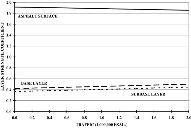
4.10 Variation of layer strength coefficients with traffic...85
Chapter 5: Specification and estimation of the roughness model based on multiple data sources...89
5.1 Joint estimation ...89
5.2 Minnesota Road Research Project (MnRoad) ...92
5.3 Measurement error model ...95
5.4 Specification of joint model ...99
5.6 Discussion of results ...106
Chapter 6: Conclusions and recommendations ...111
6.1 Concluding remarks ... 111
6.2 Concluding comments on the joint model...113
6.3 Model limitations and further research ...117
List of Figures
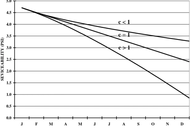
Figure 3.1: Basic proposed shape of the deterioration model based on serviceability ....43
Figure 3.2: Generic serviceability loss rate as a function of pavement strength...50
Figure 3.3: Averaged observed effect of frost depth on deterioration at AASHO ...52
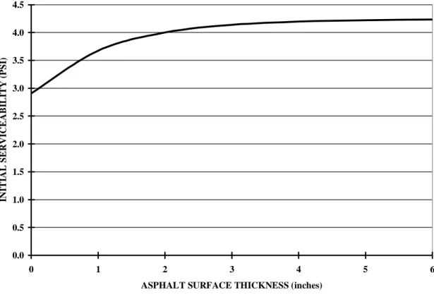
Figure 4.1: Variation of the initial serviceability with asphalt surface thickness ...76
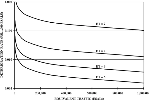
Figure 4.2: Deterioration rate as a function of strength and traffic ...77
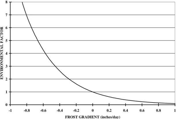
Figure 4.3: Variation of environmental factor (Fe) with frost gradient (G)...79
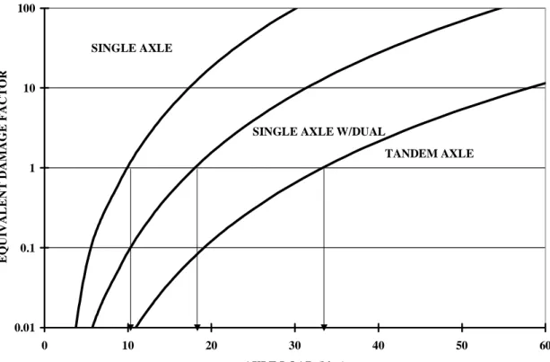
Figure 4.4: Equivalent Damage Factors (EDFs) and equivalent loads ...80
Figure 4.5: Observed and predicted serviceability for a rehabilitated section...84
Figure 4.6: Change in the value of strength coefficients with traffic ...87
Figure 5.1: Empirical relationship between roughness and serviceability ...97
Figure 5.2: Observed versus predicted performance by the linear and the nonlinear models (6,000 lbs single rear axle)...104
Figure 5.3: Observed versus predicted performance by the linear and the nonlinear models (24,000 lbs tandem rear axle)...105
Figure 5.4: Variation of the rate of roughness increase as a function of traffic, pavement strength and environmental conditions ...110
List of Tables
Table 2.1: Methods and equipment for measuring riding quality ...14
Table 3.1: Axle configuration and axle loads during the AASHO Road Test...39
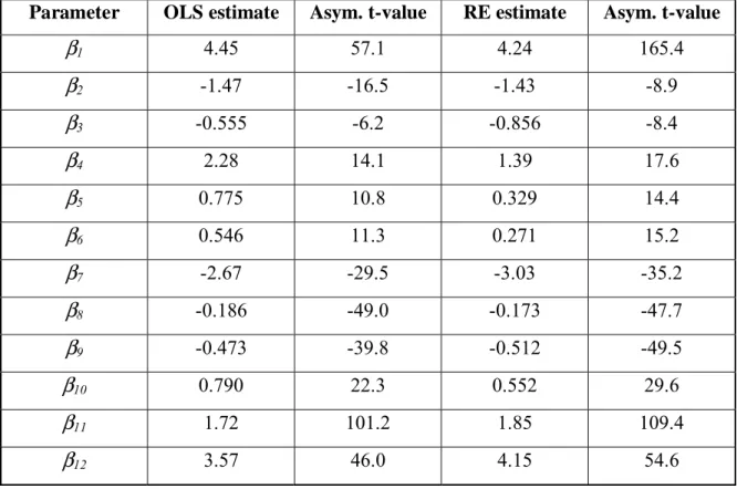
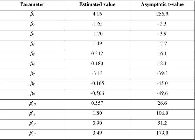
Table 4.1: Parameters and asymptotic t-values for the OLS and RE estimation ...74
Table 4.2: Estimated parameters for the serviceability model with an overlay ...83
Table 4.3: Estimated parameters for the modified model...88
Table 5.1: Axle load distribution for the experimental traffic at MnRoad ...93
Table 5.2: Parameter estimates of the joint model and corresponding t-values...103
Table 5.3: Comparison of the corresponding parameters (for the determination of equivalent traffic) of the serviceability and roughness models...106
Table 5.4: Comparison of corresponding layer strength parameters of materials used at the AASHO Road Test and at MnRoad Project ...109
Acknowledgment
I wish to express my sincere gratitude to my advisor, Professor Samer M. Madanat, for his continuous support and encouragement during my studies. This dissertation would have never been possible without his guidance and valuable advice.
I also want to express my most sincere appreciation to Professor John T. Harvey for his advice, support and friendship. Many thanks also to Professor John A. Rice for his valuable suggestions and for being always available on short notice.
My good friends Ricardo Archilla and Da-Jie Lin deserve special mention for their support and for being always available for having a “philosophical coffee break” when it was most needed.
Transportek of CSIR is deeply acknowledged for giving me the opportunity to come to Berkeley. I want to recognize the University of California Transportation Center (UCTC) for providing financial support during my final year, and the personnel of the MnRoad Project for providing the necessary data for carrying out my research and for being always ready to answer my questions.
Finally, I am grateful to my whole family, which, although at a distance, was always there for me. In particular I acknowledge my wife Jolanda who held my hand through the smooth and the rough patches of this road.
Chapter 1: Introduction and Objectives
1.1 Background
A road pavement continuously deteriorates under the combined actions of traffic loading and the environment. The ability of the road to satisfy the demands of traffic and the environment over its design life is known as performance. The most common indicators
of pavement performance are: fatigue cracking, surface rutting, riding quality, and skid resistance. The change in the value of these performance indicators over time is referred to as deterioration.
This research focuses on a methodology to develop models to predict the deterioration of the riding quality of road pavements as a function of traffic characteristics, pavement properties and environmental conditions. Hence, pavement performance is herein defined as the history of the deterioration of the riding quality.
Riding quality, per se, is a fairly subjective measure of performance. It not only depends on the physical characteristics of the pavement (surface unevenness) and the mechanical properties of the vehicle (mass and suspension), but also on the users’ perception of acceptable pavement quality. For instance, at any point in time, the riding quality of a given pavement section can be perceived differently by different road users. Moreover, riding quality expectations of a given user can be different at different points in time.
The first comprehensive effort to establish an objective indicator of pavement
performance was made in the late 1950s. Until that time, inadequate attention had been paid to the evaluation of pavement performance: a pavement was considered to be either satisfactory or unsatisfactory (Haas et al, 1994).
The Present Serviceability Index (PSI) was developed in the early 1960s and constituted the first comprehensive effort to establish performance standards based upon
considerations of riding quality (Carey and Irick, 1960; Highway Research Board, 1962). A panel of highway users from different backgrounds evaluated seventy-four flexible pavement sections and rated them on a five-point discrete scale (0 for poor, 5 for
excellent). This rating was averaged for each section converting the discrete rating into a continuous rating referred to as the Present Serviceability Rating (PSR).
The PSR was found to correlate highly with longitudinal profile variation in the
wheelpath (slope variance), and to a lesser extent with rut depth, cracking and patching. Ninety five percent of the change of the PSR could be explained by the variation of the slope variance (Haas et al, 1994). Therefore, an empirical equation was developed to determine serviceability as a function of surface slope variance, cracking, rutting and patching measured in the pavement section. The serviceability value estimated with this equation was called the Present Serviceability Index (PSI). Thus, serviceability became the first objective measure of performance based upon considerations of riding quality.
riding quality. Some of the most well-known concepts that have been developed are: the Riding Comfort Index (RCI) (CGRA, 1965), the International Roughness Index (IRI) (Gillespie et al, 1980; Sayers et al, 1986), and the Pavement Condition Index (PCI) (Shahin and Kohn, 1979). To date, the International Roughness Index has enjoyed the broadest application and has been adopted as a standard for the Federal Highway Performance Monitoring System (FHWA, 1987).
The IRI is a summary statistic of the surface profile of the road and is computed from the surface elevation. It is defined as the average rectified slope, which is the ratio of the accumulated suspension motion to the traveled distance obtained from a mechanical model of a standard quarter car traveling over the road profile at 80 km/h (Huang, 1993).
1.2 Research goal and objectives
The goal of this research is to develop a methodology for developing sound pavement riding quality deterioration models to be used primarily for the management of the road infrastructure. Ideally, these performance models could also be used for the design and analysis of flexible pavements. The accurate prediction of pavement performance is important for efficient management of the transportation infrastructure. By reducing the prediction error of pavement deterioration, agencies can obtain significant budget savings through timely intervention and accurate planning (Madanat, 1993). This is especially important since the road infrastructure network is usually the single most expensive asset owned by a local government.
At the network level, pavement performance prediction is essential for adequate activity planning, project prioritization and budget and resource allocation. At the project level, it is important for establishing the specific corrective actions needed, such as maintenance and rehabilitation.
To achieve the above-mentioned goal the following objectives should be accomplished for this research:
(i) The first objective is to development of accurate deterioration models for
predicting the riding quality of flexible pavements. These models should be based on the most reliable and comprehensive experimental data sources available. The models should incorporate the effects of the structural characteristics of the pavement, as well as the characteristics of the traffic and environmental conditions. The specification of the model should be based on sound engineering principles, and the estimation of the models should be carried out following rigorous statistical techniques.
(ii) The second objective is to transfer the deterioration models developed with
experimental data to actual traffic and environmental conditions. Transferability (or model updating) will be accomplished by joint estimation of the models using
experimental and field data. By jointly estimating the parameters of the models, the effect of new variables can be assessed and the efficiency of the parameters is improved.
Furthermore, possible biases in the experimental model can be determined and corrected.
(iii) The third objective is to validate the jointly estimated models by applying the
models to alternative data sources. Validation is accomplished by assessing the accuracy of the predictions of the updated models. Alternatively, a sample of data from the original source that was not used for the estimation of the models can be used for validation.
Pavement deterioration models are not only important for highway agencies to manage their road network, but also in road pricing and regulation studies. Both the deterioration of the pavement over time and the relative contribution of the various factors to
deterioration are important inputs into such studies. Useful models should be able to quantify the contribution to pavement deterioration of the most relevant variables. Some of the most important variables that should be accounted for are: the pavement structure (materials and strength), traffic (axle configuration and axle loads), environment
conditions (temperature and moisture) and any other factors that are relevant for cost allocation.
1.3 Research contributions
The main contribution of this research is not the development of a deterioration model, but rather the demonstration of the feasibility of using joint estimation and its many advantages, such as: (i) identification and quantification of new variables, (ii) efficient parameter estimates, (iii) bias identification and correction, and (iv) use of a measurement error model to combine apparently incompatible data sources.
The most important characteristics of the updated model to predict pavement deterioration in terms of roughness can be summarized as follows:
(i) The updated model predicts roughness incrementally and thus is ideally suited for use within a pavement management context.
(ii) The estimated exponent of the power law indicates that currently used values overestimate the equivalent traffic of the higher load classes, but underestimate the equivalent traffic of the lower load classes.
(iii) The specification allows the determination of equivalent axle loads for different configurations. These estimates revealed that the practice of using the same equivalent load for different axle configurations leads to gross estimation errors of equivalent traffic.
(iv) The specification of pavement strength in terms of the equivalent thickness allows for the determination of the relative contribution of the various materials to the overall pavement strength, even when these material have been used in different experiments.
(v) Another unique feature of the roughness prediction model is the estimation of the effect of the initial thickness of the asphalt surface on the value of the initial roughness.
(vi) The model indicates that, ceteris paribus, the rate of roughness progression decreases with traffic.
1.4 Dissertation layout
A brief introduction to pavement deterioration was given in the present Chapter together with the goals and objectives of this dissertation.
Chapter 2 contains the literature review. The significance of riding quality as a
performance indicator is discussed and some basic definitions are given. Thereafter, some important characteristics of the data sources used for the development of deterioration models are presented and discussed. This discussion is followed by a brief summary of current modeling approaches. The empirical and mechanistic approaches are discussed and their main advantages and disadvantages are highlighted. Chapter 2 concludes with a discussion of current deterioration models.
The main characteristics of the experimental data source, - the AASHO Road Test - are discussed in Chapter 3. Once the data source is described, the basic specification of the proposed deterioration models is given. This is followed by a detailed description of the various components of the model. The Chapter concludes with the formulation of the final specification form for the deterioration model in terms of serviceability (hereafter referred to as the serviceability model).
Chapter 4 deals with the estimation of the serviceability model. The Chapter begins with a discussion of basic concepts of linear and nonlinear estimation. This is followed by a discussion on the use of ordinary least squares (OLS) and random effects (RE) estimation
to deal with panel data sets. This chapter concludes with the discussion of three
serviceability models. The first model corresponds to the basic specification developed in Chapter 3. The second model is an extension of the basic serviceability model to take into account the performance of the section before and after rehabilitation. The third model extends the basic serviceability model to represent the change of the equivalent thickness of the various pavement layers with time and traffic.
The basic principles of joint estimation are presented in Chapter 5. Some of the main advantages of the technique are discussed. Thereafter, the second data source, -Minnesota Road Research Project (MnRoad)-, is discussed and its main characteristics are
presented. This is followed by a discussion on the use of a measurement error model to take into account that the observations of riding quality in the two data sources are recorded in terms of serviceability (AASHO) and roughness (MnRoad). Finally the joint model (in terms of roughness) is given, the parameters of the new model are estimated and the results are discussed.
Chapter 6 presents the conclusions of the dissertation and some recommendations. Finally, some ideas are presented with respect to the future directions of this line of research.
Chapter 2: Literature Review
This Chapter begins with a discussion of the significance of riding quality as a
performance indicator, before presenting basic definitions of riding quality and roughness in Section 2.2. A summary of riding quality measurement devices is presented in Section 2.3. This is followed by a discussion of the data characteristics that need to be considered for developing deterioration models. The empirical and the mechanistic approaches to model development are briefly discussed, and their respective advantages and
disadvantages are highlighted. Finally, the Chapter concludes with a summary of existing deterioration models and their main characteristics.
2.1 Significance of riding quality
An acceptable riding quality is important for both the road user and the goods being transported. Riding quality affects the comfort of the user for whom the road is provided, and the smoothness with which goods are moved from one point to another. If the riding quality is inadequate, goods could deteriorate in transit resulting in partial or total loss of their economic value. It is thus of economic importance that a paved road will provide adequate riding quality conditions. For this reason pavements are designed to ensure a minimum level of service over their design life. This minimum level of service can be maintained by following different maintenance and rehabilitation (M&R) strategies. The selection of a M&R strategy is based on life-cycle cost analysis of various alternatives.
From the Pavement Engineering point of view, riding quality is a function of the interaction between the longitudinal profile of the pavement and the dynamic
characteristics of the vehicles that use that pavement. Hence, vehicles affect pavement deterioration and deterioration affects vehicles, road users and goods in transit.
Riding quality also has other economic implications that are as important as the users’ riding quality considerations. Vehicle operating costs and the costs of transporting goods increase as the road riding quality deteriorates. These costs are often one order of
magnitude more important than the cost of maintaining the road to an acceptable level of service (Paterson, 1987; GEIPOT, 1982). However, while the costs of maintaining the road are usually incurred by the highway agency, the road users collect the benefits of high riding quality. While maintenance costs are usually included in a life-cycle cost analysis to determine the most economic level of service, the incurrence of vehicle
operating costs are often ignored. Previous studies have determined that vehicle operating costs (VOC) typically increase by 2 to 4 percent for each one m/km of IRI in roughness over the range of good to poor conditions (Paterson, 1987). The range for typical paved road pavements is between 2 and 10 m/km IRI.
Despite its economic importance, riding quality is not the most commonly modeled performance indicator for flexible pavements. The most common pavement deterioration models use surface rutting and fatigue cracking as performance indicators, and, to a lesser extent skid resistance.
Rutting is very important because of its safety implications. Rutting in the wheel paths allows water to pond on the surface of the pavement. A vehicle entering this area at normal highway speed may loose contact between the tire and the pavement surface, experiencing hydroplaning. This, in turn, may result in the loss of steering control of the vehicle and result in an accident. Rutting is caused by shear and densification of the pavement layer materials and subgrade.
Cracking, on the other hand, is important from a structural point of view. When cracking of the impervious surface occurs, water may enter the lower untreated layers of the pavement, weakening them. This results in loss of support of the surface layer, which accelerates the deterioration process. Cracking will progress rapidly, causing rutting and potholes to develop. The occurrence of cracking (crack initiation) is a structural problem that, in general, does not affect riding quality. However, it may trigger the acceleration of the deterioration process, as indicated above.
The skid resistance performance of the road is important because of the safety implications. To ensure safe driving conditions, the skid resistance of the pavement surface should be maintained above a minimum threshold.
Riding quality, on the other hand, allows for the economic quantification of the pavement deterioration process. Previous studies (Paterson, 1987; GEIPOT, 1982) have shown that riding quality is the most relevant road performance indicator to be considered when road performance standards are evaluated from an economic point of view. To establish a
relevant measure for riding quality, three main elements should be taken into account: (i) the surface profile of the pavement (unevenness), (ii) the dynamic characteristics of the vehicles carrying passengers or goods, and (iii) the road user.
2.2 Basic definitions
In the literature, the terms riding quality and roughness are sometimes used as opposites.
Strictly speaking from the Pavement Engineering point of view, the term roughness is linked to the quality of the road surface profile. It describes the unevenness of the road surface without considering vehicle interaction or users’ perceptions.
According to the American Society for Testing and Materials (ASTM, specification E867-82A), roughness can be defined as: “the deviations of the surface from a true planar surface with characteristic dimensions that affect vehicle dynamics, ride quality,
dynamic loads and drainage”. After the development of the International Roughness
Index (IRI) (Gillespie et al, 1980; Sayers et al, 1986) the term roughness has also been used to refer to the measure of the riding quality in terms of IRI. Subsequently, almost any measure of riding quality or IRI roughness is generally referred to as roughness. In this dissertation, riding quality will, however refer to any measure of the road conditions as perceived by the user, while roughness will be reserved for the cases when that measure is expressed in terms of IRI. The term serviceability will refer to the measure of riding quality in terms of PSI. Finally, the term unevenness will refer to the quality of the surface profile.
2.3 Equipment for measuring riding quality
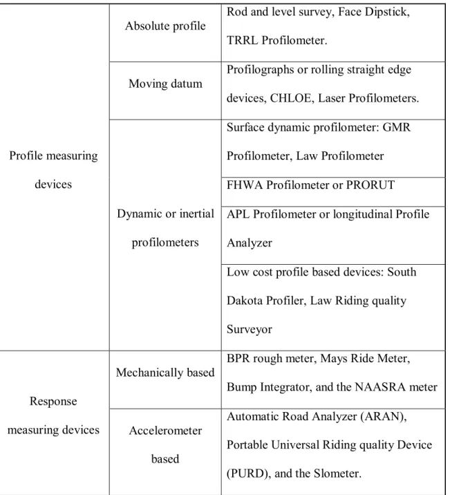
Riding quality measuring devices can be classified as profile-measuring or response-measuring devices. Table 2.1 provides a summary of the most commonly available
devices for measuring riding quality.
Profile measuring devices can be classified into three groups: (i) instruments that measure the elevation profile relative to a true horizontal datum, (ii) instruments that measure the road profile relative to a moving datum, and (iii) dynamic profile instruments or
profilometers. These devices measure the unevenness of the surface.
Response-measuring devices measure the response of the vehicle to the unevenness of the pavement. These devices can be classified into two groups: (i) devices that measure relative displacement between axle and body of the vehicle, and (ii) devices that measure accelerations of vehicle axle or body by accelerometers and integrate the signal.
Although response-type devices do not measure the surface profile but the response of the vehicle to the surface unevenness, they have been widely used by highway agencies due to their relatively low cost, simple design and high operating speed. This is possible because there are a number of empirical relationships that correlate unevenness statistics with response-type statistics.
Table 2.1: Methods and equipment for measuring riding quality.
Absolute profile
Rod and level survey, Face Dipstick, TRRL Profilometer.
Moving datum Profilographs or rolling straight edge devices, CHLOE, Laser Profilometers. Surface dynamic profilometer: GMR Profilometer, Law Profilometer FHWA Profilometer or PRORUT APL Profilometer or longitudinal Profile Analyzer
Profile measuring devices
Dynamic or inertial profilometers
Low cost profile based devices: South Dakota Profiler, Law Riding quality Surveyor
Mechanically based BPR rough meter, Mays Ride Meter, Bump Integrator, and the NAASRA meter Response
measuring devices Accelerometer based
Automatic Road Analyzer (ARAN), Portable Universal Riding quality Device (PURD), and the Slometer.
Independently of the type of device used, profile-related statistics can be classified into three categories (Sayers et al, 1986). In the first category, the full pavement surface profile is mathematically processed to predict vehicle response.
In the second category, the summary statistic is an estimate of the response of a particular piece of equipment by correlation to a waveform statistic taken from one or more selected wavelengths within the full spectrum. The third category offers more flexibility because the effects across the full spectrum can be evaluated by defining riding quality with respect to different wavelengths. The advantage of using individual wavelengths is that specific effects can be isolated and their effect on pavement performance can be assessed individually. Humans and goods respond more negatively to certain wavelengths and are more immune to others. According to a study by the World Bank (Paterson, 1987): (i) short wavelength unevenness represents defects in the upper pavement layers, (ii) medium wavelength unevenness represents defects deriving from the pavement lower layers, and (iii) long wavelength unevenness represents subsidence or heave deriving from the subgrade.
2.4 Characteristics of the data sources
The importance of an adequate data source deserves to be given some consideration. A number of possible data sources have been used over the years to develop pavement deterioration models. Some of these sources are: (i) randomly selected in-service pavement sections, (ii) in-service pavement sections selected following an experimental design, (iii) purposely built pavement test sections subjected to the action of actual highway traffic and the environment, and (iv) purposely built pavement test sections subjected to the accelerated action of traffic (for example the use of the Heavy Vehicle Simulator (HVS)) and environmental conditions (for example rapid aging by the
application of UV radiation).
Due to the nature of the pavement deterioration process, data from actual in-service pavement sections subjected to the combined actions of highway traffic and
environmental conditions are desirable. All other data sources produce models that are likely to suffer from some kind of biases or restrictions unless special considerations are taken into account during the parameter estimation. Some of these considerations are briefly described in the following paragraphs.
The most common problems encountered in models developed from randomly selected in-service pavement sections are caused by: (i) the presence of multi-collinearity between relevant explanatory variables, (ii) the unobserved events typical of such data sets, and (iii) the problem of endogeneity bias caused by the use of endogenous variables as independent explanatory variables. These are discussed separately below.
The problem of multi-collinearity is typical of time-series pavement performance data sets. Variables such as pavement age and accumulated traffic are usually almost perfectly collinear. Hence, the estimated models usually fail to identify the effects of both variables simultaneously. There are no statistical methods to address the problem of
multi-collinearity because it is a problem inherent to the data set. A typical solution consists of obtaining more data from the original source or to combine various data sources
Data gathering surveys during experimental tests are usually of limited duration. Thus, if only the events observed during the survey are considered in the statistical analysis (ignoring the information of the after and before events), the resulting models would suffer from truncation bias. If the censoring of the events are not properly accounted for, the model may suffer from censoring bias (Paterson, 1987; Prozzi and Madanat, 2000).
Another common problem is endogeneity bias. Pavements that are expected to carry higher levels of traffic during their design life are designed to higher standards. The bearing capacity of these pavements is higher than those designed to withstand lower traffic levels. Thus, any explanatory variable that is an indicator of a higher bearing capacity, such as the structural number, will be an endogenous variable that is determined within the model and cannot be assumed to be exogenous. If such a variable were
incorporated into the model, the estimated parameters would suffer from endogeneity bias (Madanat et al, 1995). Another case of endogeneity bias occurs when maintenance (which is triggered by the condition of the pavement) is used as an explanatory variable (Ramaswamy and Ben-Akiva, 1990).
The latter two problems can be addressed using statistical techniques that take into account the presence of truncation or endogeneity or, alternatively, by developing models that are based on data from in-service pavement sections that have been selected based on an experimental design.
subjected to the action of actual traffic and the environment are the best possible sources of data. However, time and budget limitations constrain this type of experiment to a very limited number (e.g., LTPP and Mn/Road High Volume facility). Building pavement test sections and subjecting them to the accelerated action of traffic and the environment solves some of the budget and time constrains (e.g. HVS, Westrack, NCAT, MnRoad Low Volume facility). Accelerated Pavement Testing (APT) facilities also may have mechanical limitations such as the maximum speed of the testing carriage. Thus, this produces models that may be conditional on the testing conditions.
One way of overcoming some of these limitations is through the use of data from multiple sources. Archilla and Madanat (2001) have successfully developed models to predict pavement rutting by combining two different data sources. Both data sources used in his dissertation correspond to experimental test sections. Thus, the models are
conditional on the experimental traffic. The next logical step in this line of research is to investigate the transferability of these models to actual mixed highway traffic
2.5 Modeling approaches
Pavement performance models can be categorized into two main groups: empirical models and mechanistic models, depending on the approach followed to develop the performance function. A third group comprises the so-called mechanistic-empirical models that use both mechanistic concepts and empirical methods. Some of the main characteristics of each type are described in the following paragraphs.
Empirical models. In empirical models, the dependent variable is any pavement
performance indicator of interest. Both aggregate indicators of performance (such as the Present Serviceability Index (PSI), the Riding Comfort Index (RCI), or the Pavement Condition Index (PCI)) and individual performance indicators (such as skid resistance, rutting, or cracking) have been used as dependent variables. These dependent variables are related to one or more explanatory variables representing pavement structural strength, traffic loading, and environmental conditions.
In some of these models, explanatory variables are used and discarded solely based on considerations of availability and the statistics of their parameters. Often, relevant variables are discarded due to low statistical significance (usually based on the t-statistic of the corresponding parameter). On the other hand, irrelevant variables are often
incorporated into the model based on the same considerations. Any model developed following such an approach will undoubtedly suffer from specification biases.
Furthermore, most of the specifications available in the literature are just linear
combinations of the available regressors. The criterion typically used to select the best specification form among several alternatives is to obtain the best possible fit to the data (usually measured by the coefficient of determination, R2).
In the better empirical models, the specification forms are based on physical laws, or at least, they intend to simulate the actual physical process of deterioration. The
phenomenon), is not constrained to linear equations. Furthermore, relevant regressors, whose parameters are not statistically significant for the given sample, remain in the specification independently of their t-statistics.
Mechanistic models. Mechanistic models are based on a physical representation of the
pavement deterioration process. However, due to the complexity of the road deterioration process, this approach is, at present, unfeasible. These deterioration models rely on the use of material behavior and pavement response models, which are believed to represent the actual behavior of the pavement structure under the combined actions of traffic and the environment. These behavior and response models are used to estimate strains, stresses and deflections at various locations in the pavement structure. These critical responses are, in turn, used to predict performance in terms of surface deformation (rutting) and crack propagation (fatigue cracking).
Although there have been various attempts, a comprehensive and reliable model that is purely mechanistic is still to be developed. Material behavior and pavement response models presently used are very simplistic and only represent material and structural responses under restricted conditions.
Mechanistic-empirical models. These models use material characterization (usually
laboratory testing) and pavement response models (usually linear elastic or finite element type models) to determine pavement response. This constitutes the mechanistic
correlated with pavement performance and finally calibrated to an actual pavement structure. Pavement test sections are used for this purpose as well as in-service pavement sections. This part constitutes the empirical component.
The calibration of these types of models to actual pavement performance is usually done by applying a bias correction factor, usually referred to as the shift factor (Queiroz, 1983;
Theyse et al, 1996; Prozzi and de Beer, 1997; Harvey et al, 1997; Timm et al, 2000). To date the determination of this factor is performed by ad-hoc procedures that are not supported by rigorous statistical analyses, or based on correlations with limited data.
Empirical and mechanistic-empirical models are currently the most widely used deterioration models despite their limitations. Empirical models based on regression analysis have been used for many years and constitute some of the most widely used deterioration models. However, over the past 20 years there has been a tendency for road agencies to direct their efforts toward mechanistic-empirical models because of the appeal from an engineering point of view.
The main advantage, which mechanistic-based models claim, is their ability to extrapolate predictions out of the data range and conditions under which they were calibrated, thus, producing deterministic performance predictions. This advantage constitutes, in turn, their main disadvantage since it is impossible to assess the reliability of the predictions when these models are used out of the original data range for which they have been calibrated.
2.6 Existing models
Linear models based on experimental data. The first pavement performance model was
developed based on the data provided by the AASHO Road Test, which took place in Illinois (HRB, 1962). The AASHO equation estimates pavement deterioration based on the definition of a dimensionless parameter g referred to as damage. The damage
parameter was defined as the loss in the value of the Present Serviceability Index (PSI) at any given time:
ω ρ = − − = t f t t N p p p p g 0 0 (2.1) where
gt : dimensionless damage parameter,
pt : serviceability at time t (in PSI units),
p0 : initial serviceability at time t = 0,
pf : terminal serviceability,
Nt : cumulative number of equivalent 80 kN single axle loads applied until
time t, and
ρ, ω : regression parameters.
By substituting pt = pf, it can be seen that ρ = Nt at failure. This deterioration model was
estimated based on data obtained from AASHO Road Test. The data from the AASHO Road Test provided little information on long-term environmental effects and no direct
information on the pavement response and performance under actual highway traffic.
The parameters ρ and ω were obtained for each pavement test section by applying Equation (2.1) in a step-wise linear regression approach. Some of the details of the approach followed are not very clear in the literature. Once the values of ρ and ω were estimated, the estimated values were expressed as a function of design and load variables, and two new linear regressions were carried out. The assumed relationship between ω
and these variables was (HRB, 1962):
3 1 2 2 4 3 3 2 2 1 1 2 1 0 0 ) ( ) ( β β β β ω ω L a D a D a D a L L + + + + + = (2.2) where L1 : axle load,
L2 : 1 for single axle vehicles, 2 for tandem axle vehicles, ω0 : a minimum value assigned to ω,
β1-β3 : regression parameters,
a1-a4 : regression parameters that were obtained by performing analyses of
variance, and
D1-D3 : thicknesses of the surface, base and subbase layer, respectively.
The specification form for the relationship between ρ and the design and load variables was the following (HRB, 1962):
2 3 1 ) ( 1 2 2 0 β β β β ρ L L L D + = (2.3) where
D : a1 D1 + a2 D2 + a3 D3 + a4 , represents the structural number (SN), and β1-β3 : regression parameters (not necessarily the same as in Equation 2.2).
In addition to being rather ad hoc, the statistical approach used to estimate the model parameters has several flaws. The most serious was the improper treatment of censored observations: pavement sections that had not failed by the end of the experiment were ignored in the estimation of the parameters of Equations (2.1) to (2.3). Moreover, Equations (2.2) and (2.3) are mis-specified because the term (L1 + L2) is the sum of a
load variable and a dummy variable, thus adding variables with different units.
Despite the identified shortcomings of the model specification and the estimation
approach, Equation (2.1) (or a modification of it) has been used as the basis for pavement design for approximately 50 years (AASHTO, 1981, 1993). This is probably because the AASHO Road Test is the most comprehensive and reliable data source available to date. Besides, the pavement test sections were conceived following a proper experimental design, thus overcoming many of the data limitations usually encountered with data from in-service pavement sections.
Linear models based on field data. A study conducted by the Transportation Road
provided the additional data needed to update the AASHO models to establish the relationship between pavement riding quality, pavement strength and actual highway traffic (Hodges et al, 1975; Parsley and Robinson, 1980). The use of in-service
pavements made it possible to improve over the original AASHO models. Some of these improvements are the incorporation of (i) mixed traffic loading, (ii) different pavement structures over different subgrades, and (iii) a variety of pavement ages. Furthermore, instead of using serviceability as a measure of riding quality, actual measurements of roughness in terms of IRI were used. The following model was developed:
t
t R f SN N
R = 0 + ( ) (2.4)
where
Rt : roughness at time t,
R0 : initial roughness at time t = 0,
f(SN) : a function of the structural number SN,
SN : structural number developed during the AASHO Road Test (denoted by D in Equation 2.3 above), and
Nt : cumulative number of equivalent 80 kN (18,000 lbs) single axle loads
applied until time t.
Two main shortcomings have been identified with this model. First, the model was based on pavement structures that consisted of cement-treated bases in 80 percent of the
are over represented in the sample and the resulting model is biased. Besides, pavement structures tend to be lighter that those typically used in the United States. Secondly, it assumes the same initial roughness value for all pavement types. The initial roughness after construction is influenced by the type of surface. Thus, the specification should take this into consideration. Another important aspect that affects the initial roughness value is the thickness of the surface layer. As the thickness of the asphalt surface layer increases, the initial roughness after construction decreases.
There are many other examples of linear deterioration models based on field data from in-service pavements. However, many of these studies have failed to quantify the effects of pavement strength, traffic loading and pavement age (time) in the same model. This does not come as a surprise since pavements that are expected to withstand higher levels of traffic are designed to higher strength. Furthermore, cumulative traffic loading and pavement age increase almost simultaneously. This results in high correlations between these variables and therefore it is difficult to assess the individual effects simultaneously. Two different issues arise: (i) multi-collinearity resulting from correlation between two or more explanatory variables (e.g. cumulative traffic and pavement age), and (ii)
endogeneity originating from the correlation between the dependent variables and what is assumed to be an independent variable (e.g. pavement strength and pavement life).
A study of ten-year time series data by Way and Eisenberg (1980) failed to identify the effect of traffic loading or pavement strength and developed a model that related roughness to time and pavement age only. The study was based on data from 51
pavement sections in the State of Arizona. The following incremental model was developed: 2 1 β β ∆ − = ∆Rt Rt t (2.5) where
∆Rt : change in roughness level at time t, ∆t : time increment, and
β1, β2 : regression parameters that depend on environmental variables.
Even though the model fits the data very well, it suffers from important specification biases. Important explanatory variables are omitted from the specification because the sample failed to characterize their significance. Furthermore, the parameters β1 and β2
were estimated by grouping the data into categories according to environmental
conditions such as rainfall, elevation, freeze-thaw cycles and temperature. This approach, although valid, does not make optimal use of the data and produces parameters that are not efficiently estimated. The research fails to recognize that important variables that affect the deterioration process are not observed. A preferred estimation approach in this case would consist of pooling all the data together and carrying out an estimation
approach that takes into account the unobserved heterogeneity between the various pavement sections. Two such approaches are the fixed effects approach and the random effects approach (Greene, 2000).
The models described in this section are generally useful within the environment under which they have been developed but they are inadequate for generalized technical or economic evaluation of the interaction among the various factors that affect riding quality, i.e., structural properties, traffic loading, age and environmental factors.
Agencies often use regression analysis to develop performance prediction models based on data available in their Pavement Management System (PMS) database. One example of such a model was developed in Alberta (Karan, 1983) with data corresponding to 25 years of observation of riding quality, surface distress, and deflections. The model estimated during that study is:
t RCI t t t RCI RCIt =β0 +β1ln( 0)+β2ln( 2 +1)+β3 +β4 ln( 0)+β5 ∆ (2.6) where
RCIt : Riding Comfort Index (scale 0 to 10) at any age t,
RCI0 : initial RCI at t = 0,
t : age in years,
∆t : years between observations, and β1-β5 : regression parameters.
While a number of other variables were also considered, such as traffic, climate zone, and subgrade soil, only pavement age and RCI were found to be statistically significant. A possible reason is that the pavements were primarily designed in the first place for
environmental deterioration, with structural sections significantly thicker than required by traffic alone. This model is an example of statistical fitting: the explanatory variables are selected from what is available according to their statistical significance and without taking into consideration the physical causes of the deterioration process. Regressors are added and removed solely based on the value of their t-statistics, resulting in a biased model.
Similarly, the Department of Transportation of the State of Washington has developed a set of regression equations based on their long-term pavement performance database (Kay et al, 1993). The models have the following general form:
2 1
100 β tβ
PCR= − (2.7)
where
PCR : Pavement Condition Rating (scale 0 to 100), and β1, β2 : regression parameter
Recommended values for the above parameters have been estimated for Western
Washington and are dependent on the type of construction and the surface type. This is a very simplistic specification. Therefore, it has very limited applicability outside the data set from which it was developed. In this case, only one variable was found to be
statistical significant so the models suffer from serious specification biases. The parameters are estimated by grouping the data thus resulting in loss of efficiency.
Linear models based on field data and mechanistic principles. The models developed
by Queiroz (1983) represent an example of mechanistic-empirical deterioration models. In his work, 63 flexible pavement sections were modeled by means of the multi-layer liner-elastic theory. The calculated responses used in the development of the models were surface deflection, horizontal tensile stress, strain and strain energy at the bottom of the surface asphalt layer, and vertical compressive strain at the top of the subgrade material. Various models were developed to relate the simulated responses to the observed pavement conditions in terms of roughness. Regression analysis was then used to
determine the predictive equations. The specified equation for the prediction of roughness is the following: t t t ST D SEN N QI ) log log( = β0 +β1 +β2 +β3 1+β4 (2.8) where
QIt : roughness at time t as measured by the quarter car index in counts/km,
t : pavement age in years,
ST : dummy variable (0 for original surface and 1 for overlaid surfaces),
D1 : thickness of the asphalt layer,
SEN : strain energy at the bottom of the asphalt,
Nt : cumulative equivalent single axle loads up to time t, and β0-β4 : regression parameters.
This study represents one of the first attempts to incorporate mechanistic principles into the pavement performance analysis. The strain energy at the bottom of the asphalt is calculated by applying a model based on multi-layer liner-elastic theory. However, the study fails to recognize the uncertainty that is introduced into the procedure by using a multi-layer linear-elastic model to calculate pavement response. This uncertainty is not incorporated into the final model so the model produces deterministic estimations.
Nonlinear models based on field data. A comprehensive study by the World Bank
(Paterson, 1987) addressed many shortcomings of previous models by developing a number of empirical models that differ in their level of complexity, accuracy and
applicability. The main advantage of these models is the effort that was made to develop a specification that is based on the real physical phenomenon of roughness progression. Moreover, the models were not constrained to be linear and sound statistical techniques were used to estimate the parameters.
The models were based on field data from the Brazil-UNDP Road Cost Study (GEIPOT, 1982; Paterson, 1987), which incorporates a very comprehensive set of cross-sectional data on riding quality, cracking, raveling, rutting, maintenance, traffic and rainfall. Pavement types and strengths, and traffic volumes were selected according to a
factorially-designed experiment. By designing the experiment, the sample was selected to minimize the collinearity between time and traffic. The sample comprised heavier
pavements subjected to low and high traffic volumes, as well as light pavement structures subjected to high and low traffic volumes.
One of the estimated deterioration models predicts roughness increments by accounting for the interaction of various forms of distress, maintenance activities, pavement strength, traffic loading, age and environmental factors. The basic principle behind this model was that the various parameters and mechanisms that were responsible for roughness
progression could be grouped into three categories or components. This categorization was done in terms of the depth of the roughness source within the pavement structure that, in turn, relates to a specific wavelength band.
The first component relates to the surface unevenness resulting from the plastic
deformation of the pavement layers under the shear stresses applied by the traffic loading. This is generally associated with distresses occurring in the lower pavement layers. This component accounts for the effects of pavement strength, traffic loading, rutting, and also those environmental effects that relate to the shear strength of the pavement materials.
The second component includes the superficial defects such as cracking, patching, potholes, raveling, etc. This group comprises all localized surface defects that can be associated with shallow distresses originating in the upper pavement layers.
Finally, the third component comprises those environmental conditions that affect the rate of roughness progression, but that do not involve structural damage. These include
The model was estimated using nonlinear least square regression. The factors that were found to have statistically significant effects on roughness progression included: (i) rut depth variation, pavement strength, cracking, and traffic loading in the structural deformation component; (ii) cracking, patching and potholing in the surface defects component; and (iii) roughness and time in the environmental component of the model. The specified model was the following:
t R Z P C D N S e R t t t = ∆ + ∆ + ∆ + ∆ + + ∆ ∆ β1 β2 β3 β4 β5 β6 β7 (2.9) where
∆Rt : increase in roughness during time period t,
S : a function of SN, H, and C,
SN : modified structural number,
H : thickness of cracked layer,
C : percentage area cracking,
∆N : number of equivalent 80 kN single axles in period t, ∆D : increase in rut depth standard deviation,
∆C : increase in area cracking in period ∆t, ∆P : increase in area of surface patching,
Z : dummy intercept estimate for sections with potholes,
Rt : roughness at time t,
∆t : time increment used in the analysis, and β1-β7 : regression parameters.
The data and the models show that significant deterioration can occur even in the absence of structural weakness. Roughness progression follows a convex trend, with the rate of progression depending initially on the traffic loading relative to the pavement strength and on the environmental conditions.
Paterson (1987) indicated that the model fitted the data well over the wide range of observed roughness increments (up to 7 m/km IRI). This good fit was achieved by introducing many relevant variables. However, the author failed to recognize that a number of variables that were introduced into the model might not be exogenous. This is the case for the structural number that, in general, is a function of the expected traffic. Something similar occurs with the development of cracking and patching. The amount of patching is a function of the amount of cracking. Moreover, cracking progression
increases more rapidly as the dynamic load increases due to increased unevenness of the pavement surface. The same applies to the development of rutting and so on.
Despite its limitation, this model is probably one of the best pavement deterioration models available to date. A specification form was developed bearing in mind the deterioration process and not the available data. Only after the model was specified, the parameters were estimated using sound estimation techniques.
2.7 Summary
The literature review revealed that, despite the numerous deterioration models available, most of them are of limited applicability, suffer from important biases, or have been estimated using inadequate methods.
In many instances, even within a given state, pavement performance data is broken down into separate groups and different models are developed for different regions. This approach, although valid, does not make optimal use of the available data. Statistical techniques, such as fixed and random effects are available to address this unobserved heterogeneity.
Also, the vast majority of the models discussed in the literature are inherently linear (linear in the parameters). This constraint is usually placed in the specification form without any apparent reason. The only possible explanation is that the estimation of the parameters of a linear specification can be carried out using a closed form solution. However, currently any desktop computer makes the estimation of nonlinear models a trivial problem.
Another source of specification bias is due to the use of traditional forms, which are often not applicable. For instance, a common assumption in road damage prediction models is the validity of the fourth power law to determine equivalent traffic. Using this approach, traffic loads of different magnitudes and configurations are converted into an equivalent
number of 18 kips (80 kN) single axle loads (ESALs). This conversion, although
universally accepted and used, has also been extensively criticized over the past 30 years. A number of studies have shown the dependence of this formulation (specifically the value of the exponent of the power law) on the type of distress being considered and the type of pavement structure (CSRA, 1986; Christison, 1986; Prozzi and De Beer, 1997; Archilla and Madanat, 2000). It is known that parameters determined under a given set of conditions are not necessarily valid when those conditions change. A sounder approach would be to determine the exponent during the estimation process whenever the
prevailing conditions are different from those predominant during the original AASHO Road Test. Some of the most important conditions to bear in mind are, inter alias, traffic loading configuration, material types, environmental conditions, and failure criteria.
Many of the available specifications have been developed without any serious attempt to represent the physical deterioration process. Although the pavement deterioration process is very complex, the specification should at least attempt to simulate the physical process.
This dissertation presents a methodology aimed at addressing some of the above-mentioned problems and limitations.
Chapter 3: Specification of the Serviceability Models Based on the
AASHO Road Test Data Set
This Chapter describes the main characteristics of the basic pavement deterioration model that was developed using data originating from only one data source. The deterioration model is specified in terms of serviceability loss to correspond with the AASHO Road Test data set. The main characteristics of the AASHO Road Test are discussed in Section 3.1. In Section 3.2, the basic model specification is presented. Sections 3.3 to 3.6 describe specific details of the specification form, and in Section 3.7, the final specification of the serviceability model is given.
3.1 The AASHO Road Test
The AASHO Road Test was sponsored by the American Association of State Highways Officials (AASHO) and was conducted from 1958 through 1960 near Ottawa, Illinois (HRB, 1962a and 1962b). The data from this experiment constitutes the most
comprehensive and reliable data set available to date. Unfortunately, some of the original raw data have been destroyed, and only summary data tables containing average values are available.
The site was chosen because the soil in the area is representative of soils corresponding to large areas of the Midwestern United States and it was fairly uniform. The climate was also considered to be representative of many states in the northern part of the country.
The average annual precipitation in the region of the test was 34 inches (864 mm). This precipitation occurred throughout the year without a significant difference between the dry and wet season. The average temperature during the summer months was 76 °F (24 °C) while the average temperature for the winter months was 27 °F (-3 °C). The soil remained mostly frozen during the winter months with the depth of frost penetration depending on the length and severity of the cold season. The rate of frost penetration with time (hereafter referred to as the frost penetration gradient) had an important impact on the performance of the various pavement sections.
Only one subgrade material and one climatic region were evaluated during the AASHO experiment. The upper part of the embankment was constructed with a selected silty-clay material with a CBR value between 2 and 4. These values are representative of large areas in the continental United States. However, although both (climate and subgrade) conditions are typical of large areas in the United States, the use of the results outside these conditions should be subjected to detailed assessment to ascertain their
applicability. Estimation of the effects of different subgrade material and environmental conditions cannot be attained with this data set. For this purpose, new data have to be obtained.
The test tracks consisted of two small loops (numbered 1 and 2) and four large loops (numbered 3 through 6). Each loop constituted a segment of a four-lane divided highway, whose north tangents were surfaced with asphalt concrete (AC) and the south tangents with Portland cement concrete (PCC). Therefore, each loop consisted of four traffic
lanes, two with AC surfaces and two with PCC surfaces. Only the flexible pavement sections were analyzed during the research presented in this dissertation.
Only loops 2 through 6 were subjected to experimental truck traffic whose load was strictly controlled. All the vehicles assigned to any one traffic lane had the same axle arrangement and axle load configuration. Table 3.1 shows a summary of the traffic-loading configurations applied to each loop and lane.
Table 3.1: Axle configuration and axle loads during the AASHO Road Test.
Weight in kN
Loop Lane Axle
configuration* Front axle Load axle Gross weight
2 1 2 1-1 1-1 9 9 9 27 18 36 3 1 2 1-1-1 1-2-2 18 27 54 107 125 240 4 1 2 1-1-1 1-2-2 27 40 80 142 187 325 5 1 2 1-1-1 1-2-2 27 40 100 178 227 396 6 1 2 1-1-1 1-2-2 40 53 133 214 307 480 * Note: 1-1-1 indicates single front axle and two single rear axles, while 1-2-2 indicates single front axle and two tandem rear axles.
Whenever possible, the traffic moved at 35 mph (56 km/h) on the test tangents. A total of approximately 1,114,000 axle load repetitions were applied from November 1958 until
December 1960. During the experiment, the time was counted by index periods. At the end of each index period readings were taken and recorded. Each index period
corresponds to a two-week period; index period 1 started on November 3, 1958.
A total of 142 flexible pavement sections were built into the various loops. Each section covered the two lanes, and each lane was subjected to a different traffic configuration, so the total number of test sections was 284. Out of this total, there were 252 original test sections and 32 duplicate sections. Only the data corresponding to the original 252 test sections were used for the estimation of the parameters of the model. The remaining data from the 32 replicated sections were kept apart to test the validity of the estimated models. The length of the test sections corresponding to the main experimental design (Design 1) was approximately 100 feet (30 meters). In addition to the main experimental design, a number of other tests were performed, increasing the total number of flexible pavement sections to 468.
Most of the sections on the flexible pavement tangents were part of a complete
experimental design (Design 1). The design factors considered were surface thickness, base thickness, and subbase thickness. The dimensions of the main factorial designs were 3 x 3 x 3. In other words, three levels of surface thickness were combined with three different base thicknesses and three levels of subbase thicknesses. The surface thickness of the pavement sections, comprising the main experimental design, varied from 1 to 6 inches (25 to 150 mm), in intervals of one inch (25 mm). The base layer varied in
(75 mm). The thickness of the subbase layer varied from 0 (no subbase layer) to 16 inches (0 to 400 mm), in increments of four inches (100 mm).
The materials used for the construction of the AC surface, base, and subbase layers were the same for all sections. Hence, the effect of the material properties on pavement performance cannot be directly assessed from the data of the main experimental design. Other experiments aimed at assessing different surface and base materials were also conducted during the AASHO Road Test, but were not part of the main experimental design. Therefore, these data were not considered in the development of the models presented in this research.
The asphalt concrete surface layer consisted of a dense-graded mix with 5.4 percent 85-100 PEN binder content. The coarse aggregate consisted of crushed dolomitic limestone whose maximum size was ¾’ (19 mm), and the fine aggregate consisted of natural sand. The maximum size of the crushed stone of the binder coarse was one inch (25 mm), and the AC content was 4.5 percent. The base material was crushed dolomitic limestone with 100 percent passing 1 ½’ (38 mm).
The riding quality of the various sections was monitored in terms of their serviceability by means of the Present Serviceability Index (PSI). The PSI varies on a continuous scale from 5.0 PSI for sections in excellent condition to 0.0 PSI for sections in very poor condition. However, for all practical purposes the value for the serviceability rarely exceeds 4.5 PSI and hardly ever falls below 1.5 PSI. It is important to note that the value