University of South Florida
Scholar Commons
Graduate Theses and Dissertations
Graduate School
11-3-2004
Applying the Wrapper Approach for Auto
Discovery of Under-Sampling and Over-Sampling
Percentages on Skewed Datasets
Ajay D. Joshi
University of South Florida
Follow this and additional works at:
https://scholarcommons.usf.edu/etd
Part of the
American Studies Commons
This Thesis is brought to you for free and open access by the Graduate School at Scholar Commons. It has been accepted for inclusion in Graduate Theses and Dissertations by an authorized administrator of Scholar Commons. For more information, please [email protected].
Scholar Commons Citation
Joshi, Ajay D., "Applying the Wrapper Approach for Auto Discovery of Under-Sampling and Over-Sampling Percentages on Skewed Datasets" (2004).Graduate Theses and Dissertations.
Applying the Wrapper Approach for Auto Discovery of Under-Sampling and Over-Sampling Percentages on Skewed Datasets
by
Ajay D. Joshi
A thesis submitted in partial fulfillment of the requirements for the degree of Master of Science in Computer Science Department of Computer Science and Engineering
College of Engineering University of South Florida
Major Professor: Lawrence O. Hall, Ph.D. Rafael Perez, Ph.D.
Sudeep Sarkar, Ph.D.
Date of Approval: November 3, 2004
Keywords: Machine Learning, Data Mining, SMOTE, RIPPER, imbalance, C4.5, F-value © Copyright 2004, Ajay D. Joshi
ACKNOWLEDGEMENTS
I gratefully acknowledge Dr. Lawrence Hall for giving me the opportunity to work with him and guiding me through all the steps of this research work. I thank Dr. Nitesh Chawla for providing his valuable comments and suggestions. I am also grateful to Dr. Rafael Perez for providing me guidance and support during the course of my graduate studies at USF and for being on my committee. I thank Dr. Sudeep Sarkar for being on my committee and taking time and efforts to review my work. I am also indebted to my parents for their support and encouragement, and to my sister who gave me inspiration in every step.
TABLE OF CONTENTS
LIST OF TABLES ... iii
LIST OF FIGURES...v
ABSTRACT... viii
CHAPTER 1 INTRODUCTION...1
CHAPTER 2 RELATED WORK ...3
2.1. The Class Imbalance Problem and Solutions ...3
2.1.1. Over-Sampling with Re-Sampling of Minority Classes ...3
2.1.2. Under-Sampling of Majority Classes...4
2.1.3. Assignment of Different Costs for Different Misclassification Error...4
2.1.4. Learning by Recognition...5
2.1.5. Discussion...5
2.2. Synthetic Minority Over-sampling TEchnique (SMOTE) ...7
2.3. The Wrapper Approach...10
2.4. Measurements and Metrics ...11
2.5. Discussion ...13
CHAPTER 3 WRAPPER UNDER-SAMPLE SMOTE ALGORITHM ...14
3.1. Wrapper Based Algorithm to Select Under-sampling Percentages...15
3.2. Wrapper Based Algorithm to Select SMOTE Percentages ...18
3.3. Cross-Validation of System ...20
CHAPTER 4 EXPERIMENTS ...22
4.1. Datasets ...22
4.2. Machine Learning Algorithms ...23
4.2.1. C4.5...23
4.2.2. RIPPER...24
4.3. Consistency of Training, Testing and Validations Sets...24
4.4. Tests for Statistical Significance...25
4.5.1. Phoneme Dataset...27
4.5.2. Satimage Dataset...31
4.5.3. Mammography Dataset...34
4.5.4. Forest Cover Dataset...37
4.5.5. Pima Indian Diabetes Dataset ...40
4.5.6. Oil Dataset ...43
4.5.7. KDD-cup 99: Network Intrusion Detection Dataset...46
4.6. Summary ...53
4.7. Result Comparison...56
4.8. Results Using a Brute Force Search Method...58
CHAPTER 5 CONCLUSION & FUTURE WORK ...61
LIST OF TABLES
Table 2-1. Confusion Matrix Defining Four Possible Classification Scenarios...12
Table 3-1. Hypothetical Scenario 1 – Performance Metrics...16
Table 3-2. Hypothetical Scenario 2 – Performance Metrics...16
Table 4-1. Summary of Datasets ...22
Table 4-2. Results for Phoneme Dataset ...28
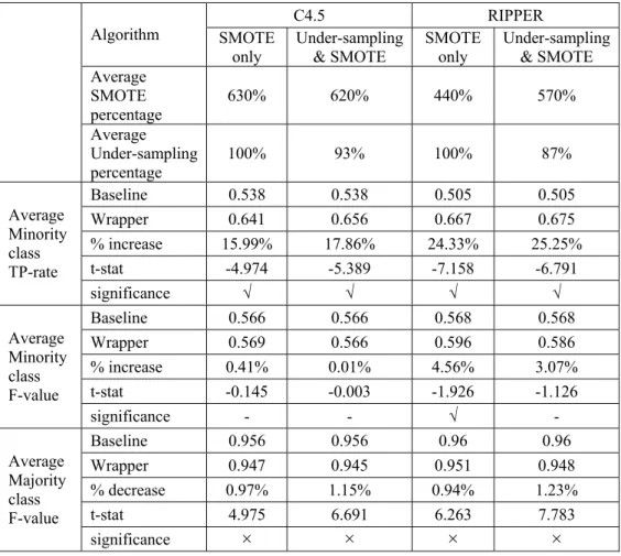
Table 4-3. Results for Satimage Dataset ...31
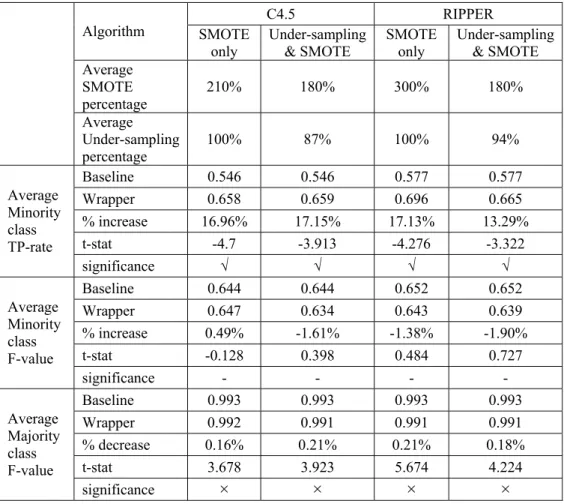
Table 4-4. Results for Mammography Dataset...34
Table 4-5. Results for Forest Cover Dataset...37
Table 4-6. Results for Pima Indian Diabetes Dataset ...40
Table 4-7. Results for Oil Dataset ...43
Table 4-8. Class Categories and Number of Examples in Original Training and Test Sets ...47
Table 4-9. Modified KDD-cup 99 Intrusion Detection Test Dataset Summary ...48
Table 4-10. Results for Modified KDD-cup 99 Intrusion Detection Dataset Using C4.5 ...48
Table 4-11. Results for Modified KDD-cup 99 Intrusion Detection Dataset Using RIPPER ...48
Table 4-12. Details of Two Versions of Original Training Data...50
Table 4-13. Cost Matrix Used for Scoring Entries in KDD Cup 99 Competition...51
Table 4-14. SMOTE Percentages Selected by Under-sample SMOTE Algorithm ...51
Table 4-15. Comparison of Results Obtained on Original KDD Cup 99 Test Data...51
Table 4-16. Significance of Improvement in TP-rate Over Minority Class ...53
Table 4-17. Statistical Significance Between ‘Smote Only’ & ‘Under-sampling & SMOTE’ ...53
Table 4-18. Winners: C4.5 Against RIPPER ...55
Table 4-19. Comparison of Hand-picked Parameters with Under-sample SMOTE Algorithm Parameters (C4.5 as base classifier) ...57
Table 4-20. Comparison of Results between Hand-picked Parameters with Under-sample SMOTE
Algorithm Picked Parameters (C4.5 as base classifier)...57 Table 4-21. Results Using Brute Force Method ...59
LIST OF FIGURES
Figure 2-1. Decision Region for Majority Class Containing Three Minority Class Examples:
Mammography Dataset ...6
Figure 2-2. Very Specific Decision Regions for Three Minority Class Examples in Solid Line Rectangular Boxes: Mammography Dataset ...6
Figure 2-3. SMOTE Algorithm ...8
Figure 2-4. The Wrapper Approach to Feature Subset Selection ...10
Figure 3-1. Wrapper Under-sample SMOTE Algorithm...15
Figure 3-2. Wrapper Under-sample Algorithm ...17
Figure 3-3. Wrapper SMOTE Algorithm ...19
Figure 4-1. True Positive Rate for Phoneme Data Using C4.5 – SMOTE with Under-sampling ...29
Figure 4-2. True Positive Rate for Phoneme Data Using C4.5 – SMOTE Only ...29
Figure 4-3. F-value for Phoneme Data Using C4.5 – SMOTE with Under-sampling...29
Figure 4-4. F-value for Phoneme Data Using C4.5 – SMOTE Only...29
Figure 4-5. True Positive Rate for Phoneme Data Using RIPPER – SMOTE with Under-sampling ...30
Figure 4-6. True Positive Rate for Phoneme Data Using RIPPER – SMOTE Only ...30
Figure 4-7. F-value for Phoneme Data Using RIPPER – SMOTE with Under-sampling...30
Figure 4-8. F-value for Phoneme Data Using RIPPER – SMOTE Only...30
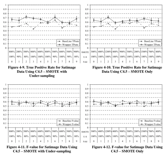
Figure 4-9. True Positive Rate for Satimage Data Using C4.5 – SMOTE with Under-sampling ...32
Figure 4-10. True Positive Rate for Satimage Data Using C4.5 – SMOTE Only ...32
Figure 4-11. F-value for Satimage Data Using C4.5 – SMOTE with Under-sampling...32
Figure 4-12. F-value for Satimage Data Using C4.5 – SMOTE Only...32
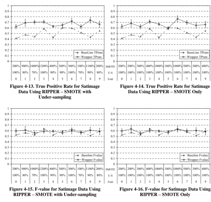
Figure 4-13. True Positive Rate for Satimage Data Using RIPPER – SMOTE with Under-sampling ...33
Figure 4-15. F-value for Satimage Data Using RIPPER – SMOTE with Under-sampling...33
Figure 4-16. F-value for Satimage Data Using RIPPER – SMOTE Only...33
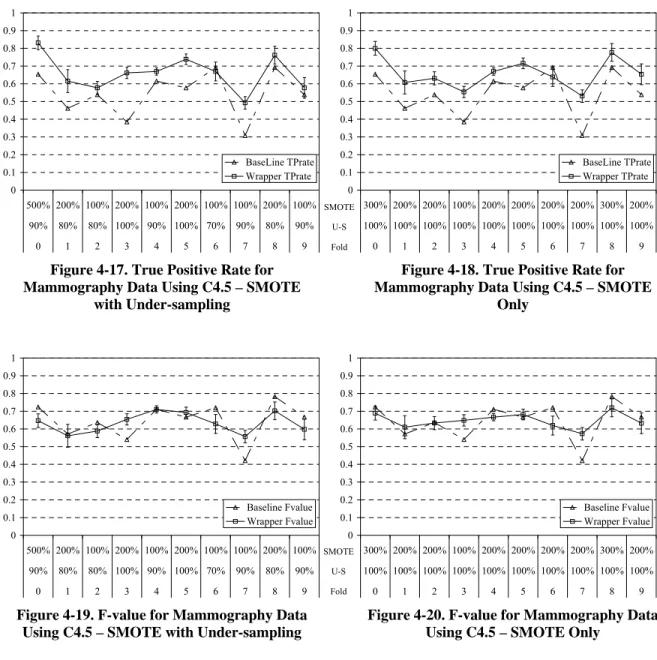
Figure 4-17. True Positive Rate for Mammography Data Using C4.5 – SMOTE with Under-sampling...35
Figure 4-18. True Positive Rate for Mammography Data Using C4.5 – SMOTE Only...35
Figure 4-19. F-value for Mammography Data Using C4.5 – SMOTE with Under-sampling ...35
Figure 4-20. F-value for Mammography Data Using C4.5 – SMOTE Only...35
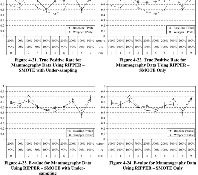
Figure 4-21. True Positive Rate for Mammography Data Using RIPPER – SMOTE with Under-sampling...36
Figure 4-22. True Positive Rate for Mammography Data Using RIPPER – SMOTE Only...36
Figure 4-23. F-value for Mammography Data Using RIPPER – SMOTE with Under-sampling ...36
Figure 4-24. F-value for Mammography Data Using RIPPER – SMOTE Only ...36
Figure 4-25. True Positive Rate for Forest cover Data Using C4.5 – SMOTE with Under-sampling ...38
Figure 4-26. True Positive Rate for Forest cover Data Using C4.5 – SMOTE Only ...38
Figure 4-27. F-value for Forest cover Data Using C4.5 – SMOTE with Under-sampling...38
Figure 4-28. F-value for Forest cover Data Using C4.5 – SMOTE Only...38
Figure 4-29. True Positive Rate for Forest cover Data Using RIPPER – SMOTE with Under-sampling...39
Figure 4-30. True Positive Rate for Forest cover Data Using RIPPER – SMOTE Only ...39
Figure 4-31. F-value for Forest cover Data Using RIPPER – SMOTE with Under-sampling...39
Figure 4-32. F-value for Forest cover Data Using RIPPER – SMOTE Only...39
Figure 4-33. True Positive Rate for Pima Data Using C4.5 – SMOTE with Under-sampling ...41
Figure 4-34. True Positive Rate for Pima Data Using C4.5 – SMOTE Only...41
Figure 4-35. F-value for Pima Data Using C4.5 – SMOTE with Under-sampling ...41
Figure 4-36. F-value for Pima Data Using C4.5 – SMOTE Only ...41
Figure 4-37. True Positive Rate for Pima Data Using RIPPER – SMOTE with Under-sampling ...42
Figure 4-38. True Positive Rate for Pima Data Using RIPPER – SMOTE Only ...42
Figure 4-39. F-value for Pima Data Using RIPPER – SMOTE with Under-sampling ...42
Figure 4-40. F-value for Pima Data Using RIPPER – SMOTE Only ...42
Figure 4-42. True Positive Rate for Oil Data Using C4.5 – SMOTE Only...44
Figure 4-43. F-value for Oil Data Using C4.5 – SMOTE with Under-sampling ...44
Figure 4-44. F-value for Oil Data Using C4.5 – SMOTE Only ...44
Figure 4-45. True Positive Rate for Oil Data Using RIPPER – SMOTE with Under-sampling ...45
Figure 4-46. True Positive Rate for Oil Data Using RIPPER – SMOTE Only ...45
Figure 4-47. F-value for Oil Data Using RIPPER – SMOTE with Under-sampling...45
Figure 4-48. F-value for Oil Data Using RIPPER – SMOTE Only ...45
Figure 4-49. Comparison of Brute Force and Heuristic Search for Wrapper True Positive Rate on Phoneme Data...59
Figure 4-50. Comparison of Brute Force and Heuristic Search for Wrapper F-value on Phoneme Data...59
Figure 4-51. Comparison of Brute Force and Heuristic Search for Wrapper True Positive Rate on Mammography Data ...60
Figure 4-52. Comparison of Brute Force and Heuristic Search for Wrapper F-value on Mammography Data...60
APPLYING THE WRAPPER APPROACH FOR AUTO DISCOVERY OF UNDER-SAMPLING & OVER-SAMPLING PERCENTAGES ON SKEWED DATASETS
Ajay D. Joshi
ABSTRACT
Machine learning applications are plagued by the imbalance observed among the class sizes in many real world datasets. A dataset is said to be skewed or imbalanced when its classes are very unequally represented. A naïve classifier learned from these skewed datasets is always biased towards the majority classes which constitute a major percentage of the samples in the dataset. As a result the accuracy on the minority classes is hampered. In many real world applications like network intrusion detection, cancer detection from mammography images, etc. the events of interest are very rare and the cost of not detecting these events is very high. Hence it very important to improve accuracies on the minority classes. It has been proposed previously that under-sampling of the majority classes can reduce the bias of the learned classifier and over-sampling of the minority classes - especially SMOTE (Synthetic Minority Over-sampling TEchnique) can boost the classifier accuracy on minority classes. But the question of how much under-sampling and over-under-sampling to be done for a particular induction learning algorithm and dataset remains. We present a wrapper approach for searching for the under-sampling and over-sampling (i.e. SMOTE) percentages for a particular learning algorithm for a given skewed dataset. We compare the results obtained by the classifiers built on wrapper selected under-sampled and SMOTEd datasets with the ones obtained by classifiers built on the original datasets to show a statistically significant improvement in accuracies over minority classes. This proves the efficacy of the wrapper approach in searching for the under-sampling and over-sampling percentages. Further, it provides an automated method to select the number of synthetic examples to be created.
CHAPTER 1 INTRODUCTION
The past decade has seen a remarkable increase in the amount of information being stored and distributed in electronic format over the internet [1]. With the increase in use of automated electronic data gathering and remote sensing devices, with the falling prices of data storage and computing power, data collection has become very cheap and has contributed to the explosion of accessible data. This has provided the Data Mining community with an exceptional opportunity for extracting nontrivial implicit information from massive datasets. In spite of this huge amount of real world data, only some of the data instances are of interest and usually they are in the minority. These data instances constitute the minority classes, while the remaining instances make up the majority classes. These kinds of datasets sets are called skewed or imbalanced datasets. Many machine learning datasets such as network intrusion detection, fraud transaction detection, medical diagnostics, etc. are hard to learn from without a significant bias towards the majority classes. In addition, many times the cost of misclassifying the interesting data instances in the minority classes as belonging to other majority classes is much higher than the cost of the reverse error.
For example, in network intrusion detection applications, where the illegal activity on the network is usually a very small percent of the normal activity, the aim of the application is to catch all network intrusions including the unseen network attacks by continuously monitoring for any unusual user activity and to keep a low false alarm rate. The issue of detecting future novel attacks has led to an escalating interest in data mining techniques for intrusion detection [2] [3] [4] [5] [6]. In the case of medical diagnosis, the cost of a false positive diagnosis generally results only in putting the patient through unnecessary medical tests whereas the result of a false negative diagnosis can be fatal. To make matters worse, normally the datasets on which medical diagnostic applications are built are also imbalanced as in the case of detecting the pixels in mammography images as cancerous or normal [7] [8] [9], where the
abnormal cancerous pixels are only a very small fraction of the total pixels. Previous studies related to fraud detection [10] have revealed an imbalance in the data of the order of 100 to 1. In some high energy physics applications [10] there is a 10,000 to 1 imbalance between the majority and minority classes. Some research in the domains of fraudulent telephone calls [11], telecommunication management [12], text classification [13] and detection of oil spills in satellite images [14] has been done to deal with the problem of imbalanced datasets. All these applications require a reasonably high detection rate for the minority classes and a minimal error rate for the majority classes.
The recent interest in the class imbalance problem has led to two special workshops held at AAAI in 2000 [15] and ICML in 2003 [16], and a special issue newsletter from SIGKDD Explorations [17] on learning from imbalanced datasets. Researchers in the machine learning community have dealt with the problem of class imbalance with various approaches like over-sampling the minority classes, under-sampling the majority classes, assigning different costs for different misclassification errors, learning by recognition as opposed to discrimination, etc. Lots of research has been done in comparing the various sampling methods and even a question of whether sampling is becoming the de facto standard for countering the imbalance in datasets has been raised in the special issue SIGKDD Explorations [17] editorial. With all this there is still no research on finding the approach to sampling required to get good classifier accuracies on minority classes. This provides us the motivation for our research.
The remainder of the thesis is organized into chapters as follows: Chapter 2 discusses some of the important previous work on the approaches used in alleviating the class imbalance problem and their limitations, the wrapper approach and its uses in different scenarios, how we intend to use wrappers and finally the performance metrics used in our study. Chapter 3 presents our wrapper Under-sample SMOTE algorithm used for finding the under-sampling and SMOTEing percentages for the skewed datasets. Chapter 4 provides a description of the datasets used in our study and presents experimental results which confirm the applicability of our approach. Chapter 5 discusses conclusions and proposes directions for future work.
CHAPTER 2 RELATED WORK
2.1.The Class Imbalance Problem and Solutions
As discussed in the Introduction chapter, the problem with the imbalanced class distribution observed in many real world data applications is significant and a lot of research has been done on this problem. The researchers have dealt with the problem of class imbalance using two main approaches. The first one is to assign distinct costs to training examples [15] [19] and the other is to re-sample the original dataset by either over-sampling or SMOTEing the minority classes and / or under-sampling the majority classes [7] [13] [20] [21] [22]. The details of these approaches and a few other important strategies are discussed in the following subsections.
2.1.1.Over-Sampling with Re-Sampling of Minority Classes
Over-sampling of minority classes can be done by re-sampling the examples from minority classes thus increasing the bias of the learned classifier towards them and increasing the accuracy on minority classes. Japkowicz [22] has experimented with over-sampling the minority classes in several artificial one dimensional datasets with varying concept complexities using multi-layered perceptrons and has found the approach effective in datasets with complex concepts. She has used two re-sampling methods, random re-sampling in which the minority class is re-sampled randomly until it consists of as many examples as the majority class and focused re-sampling in which only examples which occur on the boundary of minority and majority classes are re-sampled. Focused re-sampling was found to give no clear advantage over the random re-sampling. Similarly, Ling and Li [21] have used the over-sampling approach in the direct marketing domain. They have used ada-boosted Naïve Bayes and ada-boosted C4.5 with lift analysis as a measure of a classifier’s performance on three real world datasets: a loan product promotion dataset and two datasets one from a major life insurance company and another from a company which ran “bonus
programs”. They found that over-sampling of the minority class did not significantly improve the classifiers performance. There was some improvement for ada-boosted C4.5, but none for the ada-boosted Naïve Bayes classifier. This difference in performance for different learning algorithms shows that the amount of over-sampling done could also be a function of the type of inductive learning algorithm used to build the classifier in addition to the order of imbalance and the complexity of the dataset.
2.1.2.Under-Sampling of Majority Classes
Under-sampling the majority class can reduce the bias of the learned classifier towards it and thus improve the accuracy on the minority classes. Kubat and Matwin [20] have provided an intelligent solution for doing selective under-sampling of the majority class in a two class problem. The majority class examples are divided into four categories: safe, redundant, borderline and class-label noise examples. The redundant examples are eliminated using the 1-NN rule while the borderline and class-label noise examples are removed using the concept of Tomek links [23]. Thus this one-sided selection method removes examples from the majority class while leaving the minority class untouched. The evaluation of the trained classifiers was done using a geometric mean of accuracy on minority and majority classes. From the results, it was found that the under-sampling approach was effective, as there was a significant improvement in performance measures over most of the testbed datasets.
2.1.3.Assignment of Different Costs for Different Misclassification Error
The relative importance of different kinds of errors can be represented by a cost matrix. Suppose there are C classes, we have a C x C cost matrix, where the value in row i and column j gives the cost or loss of predicting a case to belong to class i, when it actually belongs in class j. Normally the cost is zero when i equals j and one when i is not equal to j, which gives us the normal classification error-rate. If the cost is one if i equals j and zero otherwise, then the cost measure is the common classification accuracy measure. Several studies in the literature have proposed approaches for finding optimal cost matrices which assign higher costs for misclassification of cases from minority classes and lower cost otherwise. One such study was done by Domingos, who proposed a method for making an arbitrary classifier cost-sensitive by wrapping a minimizing procedure, called MetaCost [15], around it. A close connection between cost-sensitive approaches and sampling techniques has be found by [24][25].
2.1.4.Learning by Recognition
In this approach the classification of the examples is done using a recognition-based inductive scheme instead of the discrimination-based scheme where one of the two classes is mostly ignored i.e. examples from that class are not used in the training process. Japkowicz et al. [23] have proposed a Novelty Detection technique for concept learning which proceeds by recognizing the examples from one class rather than differentiating between the examples from two classes. The approach involves training an auto-encoder – a multi-layered perceptron to reconstruct the examples from one class at the output layer and then using the auto-encoder to recognize novel examples. The auto-encoder recreates the input with small error if it belongs to the class the auto-encoder is built upon or large error if it came from the other class. Japkowicz [22] built two auto-encoders, one on the majority class and the other on the minority class but failed to reach the performance obtained by either the random over-sampling or random under-sampling approaches. Tax [26] has done similar research using SVM which was found to be competitive [27] with other recognition based learners.
2.1.5.Discussion
Some studies [21] [22] have been done which combined under-sampling of majority classes with over-sampling by replication of minority classes. While Japkowicz [22] had found this approach very effective, Ling and Li [21] were not able to get significant improvement in their performance measures. Japkowicz [22] had experimented with only one-dimensional artificial data of varying complexity whereas Ling and Li [21] had used real data from a Direct Marketing problem. This might have been the reason for the discrepancy between their results. On the whole from the body of literature, it was found that under-sampling of majority classes was better than over-sampling with replication of minority classes and that combination of the two did not significantly improve the performance over under-sampling alone.
But later, Chawla et al. [7] introduced a new over-sampling approach for a two class problem that over-sampled the minority class by creating synthetic examples rather than replicating examples. They pointed out the limitation of the over-sampling with replication in terms of the decision regions in feature space for decision trees. They concurred that as the minority class was over-sampled by increasing amounts, for decision trees, the result was to identify similar but more specific regions in the feature space
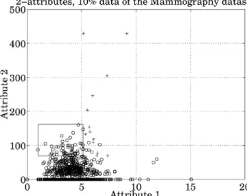
as the decision regions for the minority class. This can be observed in the decision region plots for decision trees on the mammography dataset using 2 attributes as shown in Figure 2-1 [7] and Figure 2-2 [7].
Figure 2-1. Decision Region for Majority Class Containing Three Minority Class Examples: Mammography Dataset
Figure 2-2. Very Specific Decision Regions for Three Minority Class Examples in Solid Line Rectangular Boxes: Mammography Dataset
From Figure 2-1 [7], in which the majority class samples are indicated by the ‘o’ marker and minority class samples by ‘+’ marker, the region encapsulated by the solid line rectangle is the majority class decision region. It can be seen that this region includes three minority class samples i.e. the decision tree is misclassifying those minority class samples. But when the minority class is over-sampled using replication of the minority samples, it causes more splits in the decision tree leading to more terminal nodes/leaves as
the decision tree learning algorithm tries to fit more and more similar minority class data. This results in over-fitting the data and makes the decision regions for the minority class very specific. This is evident in Figure 2-2 [7], where it can be seen that the three previously misclassified minority class samples are classified correctly, but at the expense of very specific decision regions around them. Though one gets better accuracy for minority classes on training data, this does not hold true on the unseen test data. What we want is that the decision region for the minority class spreads into the majority class region as much as possible without much reduction, if any, in majority class accuracy; and thus be able to generalize well over unseen minority class data. The new approach called Synthetic Minority Over-sampling TEchnique (SMOTE) [7] overcomes the problem of specific decision regions by creating synthetic examples in the vicinity of the present minority class examples. A detailed description of this approach for over-sampling the minority classes, which is the approach used in our study, follows in the next section.
2.2.Synthetic Minority Over-sampling TEchnique (SMOTE)
The introduction of this approach of over-sampling for the minority class was inspired by a similar technique which was successful in handwritten character recognition [29]. The over-sampling was done by selecting “each minority class example and creating a synthetic example along the line segment joining the selected example and any/all of the k minority class nearest neighbors” [7, p.328]. In the calculations of the nearest neighbors for the minority class examples “a Euclidean distance for continuous features and the value Distance Metric (with the Euclidean assumption) for nominal features” [9, p.2] was used. For examples with continuous features, the synthetic examples are generated by taking the difference between the feature vectors of selected examples under consideration and their nearest neighbors. The difference between the feature vectors is multiplied by a random number between 0 and 1 and then added to the feature vector of the example under consideration to get a new synthetic example. For nominal valued features, a majority vote for the feature value is taken between the example under consideration and its k nearest neighbors [7]. This approach effectively selects a random point along the line segment between the two feature vectors. This strategy forces the decision regions of the minority class learned by the classifier to spread and effectively provides better generalization performance on unseen data. This can be seen in Figure 2-2 [7], where the region encapsulated by the dashed line rectangle is the decision region for the
minority class. This approach also reduces the size of the decision tree as the classifier does not learn specifics of the data by reducing over-fitting.
Chawla et al. [7] experimented with a combination of under-sampling of the majority class and SMOTE for the minority class, and found that the combination of both approaches performed better than under-sampling alone. However, the question of how much under-sampling and over-sampling to be done for a given dataset was not answered and our study tries to answer this very question.
The pseudo code1 for generation of new synthetic minority class samples is shown in Figure 2-3 [9].
Figure 2-3. SMOTE Algorithm [9] AlgorithmSMOTE (T, N, k)
Input: Number of minority class samples T;
Amount of SMOTE N%;
Number of nearest neighbors k (k = 5 is used in our experiments)
Output: (N/100) * T synthetic minority class samples
1. (* If N is less than 100%, randomize the minority class samples as only a random percent
of them will be SMOTEd. *)
2. ifN < 100
3. then Randomize the T minority class samples
4. T = (N/100) * T
5. N = 100 6. endif
7. N = (int)(N/100) (* The amount of SMOTE is assumed to be in integral multiples of 100 *) 8. k = Number of nearest neighbors
9. numattrs = Number of attributes
10. Sample[][]: array for original minority class samples
11. newindex: keeps count of the number of synthetically generated samples; it is initialized to 0
12. Synthetic[][]: array of synthetic samples
(* Compute k nearest neighbors for each minority class sample only *)
13. fori← 1 toT
14. Compute k nearest neighbors for i, and save the indices in the nnarray
15. Populate(N, i, nnarray) 16. endfor
Figure 2-3. SMOTE Algorithm Contd. [9]
Populate (N, i, nnarray) (* Function to generate the synthetic samples. *)
1. whileN≠ 0 do
2. choose a random number between 1 and k, call it nn. This step chooses one of the k
nearest neighbors of i.
3. forattr← 1 tonumattrs
4. ifattr = = Continuous feature
5. Compute: dif = Sample[nnarray[nn]][attr] – Sample[i][attr] 6. Compute: gap = random number between 0 & 1
7. Synthetic[newindex][attr] = Sample[i][attr] + gap * dif
8. else
9. attr_value = majority vote for the attr value from k nearest neighbors. If no majority
then choose at random.
10. Synthetic[newindex][attr] = attr_value
11. endif
12. endfor
13. newindex++
14. N = N – 1 15. endwhile
16. return (* End of Populate *)
2.3.The Wrapper Approach
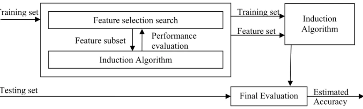
Kohavi et al. [30] were the first to introduce the wrapper approach to the mainstream Data Mining community. They successfully used the wrapper approach to search for an optimal feature subset customized to a specific induction learning algorithm and domain. The idea behind the wrapper approach is very simple and is shown in Figure 2-4, where the induction learning algorithm which is used as a black box is run repeatedly on a distinct portion of the dataset using various feature subsets. Some performance measure is used to evaluate the classifier built on each feature subset using a set aside distinct portion of the dataset, and the feature subset with the highest evaluation is used as the final set to build the final classifier on all the data instances in the training set. The resulting classifier can then be evaluated on an independent test set that is not used during the search process to assess the efficacy of the wrapper approach in selecting the feature subset.
Figure 2-4. The Wrapper Approach to Feature Subset Selection
After Kohavi et al. successfully used the wrapper approach in the feature subset selection problem, there were many researchers who experimented with the wrapper approach in various contexts. Langley and Sage [31] used the wrapper approach in selecting the features for a Naïve-Bayes classifier. Pazzani [32] created super-features by combining the base features for a Naïve-Bayes classifier by using the wrapper approach and demonstrated that it really was able to find the correct combination of features when they interacted. A significant improvement over the original K2 algorithm was shown by Singh and Provan [33]
Feature selection search
Induction Algorithm Performance evaluation Training set Training set Induction Algorithm Feature set Feature subset Final Evaluation
Testing set Estimated
when they selected the features for Bayesian networks using the wrapper approach. Again, Kohavi and John [34] demonstrated the use of the wrapper with other search methods using probabilistic estimates for feature subset selection.
Other than feature selection, the wrapper approach has been used for many other problems. Kohavi and John [35] applied the wrapper approach for tweaking the parameters of C4.5 for maximal performance. The wrapper approach was used by Skalak [36] in an interesting fashion to select the training instances (prototype subset) instead of the features in connection with nearest-neighbor classifiers.
Our algorithm, which searches for under-sampling and over-sampling percentages for minority and majority classes respectively, includes a modified version of the wrapper algorithm.
2.4.Measurements and Metrics
Traditionally, the performance evaluation of machine learning algorithms was done using just the predictive classification accuracy, which did not capture the essence of recognizing the minority classes in skewed datasets with diverse costs of errors. In skewed datasets, where the majority class constitutes about 98% - 99% of all the data instances, a trivial classifier which predicts everything as belonging to the majority class can achieve an accuracy of 98% - 99% which appears great on the surface. So it is apparent that for domains with imbalanced distributions, classification accuracy is not an appropriate performance measure. Previous studies involving imbalanced datasets have used various different performance measures suitable to this type of problem. For example, Kubat and Matwin [15] used the geometric mean of accuracies measured on the minority and majority class with the idea to improve the accuracy on both classes while keeping them balanced. But this metric did not take into account the different costs for different misclassification errors. Several studies [7] [37] [38] [39] have used ROC (Receiver Operating Characteristics) analysis as a standard technique for summarizing the classifiers performance over a range of tradeoffs between true positives and false negatives and AUC (Area Under the Curve) as the performance metric for ROC curves. In [7], for generation of ROC curves, the data set was SMOTEd for minority classes at a specific percentage while the under-sampling of the majority class was done over a range of percentages ranging from 0% to 100% to get the points on the ROC curve. Then the SMOTE percentage, which was used to SMOTE the dataset for the minority class which yielded the best AUC
measure, was selected as the best SMOTE percentage. Thus the AUC measure gives the best SMOTE percentage for an under-sampled percentage of the majority class ranging from 0% to 100%. But what we are really interested in, is the specific amount of SMOTE and under-sampling percentages i.e. a single point on the ROC curve that will give us the best tradeoff between the true positives and false positives. The AUC measure does not provide that, and so is not considered to be an appropriate performance measure here. Also the AUC measure does not take into account the cost of classifying a positive case as negative (FN) and also is very hard to extend for multiple class problems.
The F-value [40] [41] measure which takes into consideration the false positives and false negatives along with true positives was the right metric for our study. A confusion Matrix as shown in Table 2-1 is used in calculation of the F-value. In our case the minority class under consideration is deemed as the positive class, whereas all other classes together constitute the negative class.
Table 2-1. Confusion Matrix Defining Four Possible Classification Scenarios
Predicted Positive Class Predicted Negative Class Actual Positive class True Positives (TP) False Negatives (FN) Actual Negative Class False Positives (FP) True Negatives (TN)
The F-value metric incorporates two other measures: Precision which gives us the measure of correctness of the classifier in predicting the actual positive or minority class, whereas Recall gives us the measure of the percentage of positive or minority class examples predicted correctly. Using the Table 2-1, Precision, Recall and F-value are calculated as follows:
(FP) Positives False (TP) Positives True (TP) Positives True Precision + = (2.1) (FN) Negatives False (TP) Positives True (TP) Positives True Recall + = (2.2) Precision Recall Precision Recall ) (1 value -F 2 2 × × × × + = β β (2.3)
Where β controls the relative importance assigned to recall and precision.
For any machine learning algorithm, it is desirable to improve the recall without sacrificing the precision. However, the optimal independent parameter settings to optimize for Recall or Precision are
often conflicting and optimizing both of them simultaneously may be difficult. Both of these measures are included by the F-value and so the goodness of the classifier can be measured by the F-value.
2.5.Discussion
From the previous research on boosting accuracy for minority classes, a combination of over-sampling of minority classes using SMOTE and under-sampling of majority classes has been found effective. However, a method to find how much to SMOTE and under-sample is still not known. The wrapper approach has been successfully used in many domains viz. searching for the optimal feature subset, tuning parameters of induction learning algorithms, etc. So in this study we have used the wrapper approach in searching for SMOTE percentages for minority classes and under-sampling percentages for majority classes, guided by the F-value as a performance metric, for a specific induction learning algorithm on imbalanced datasets. The next chapter presents the Wrapper Under-sample SMOTE algorithm.
CHAPTER 3
WRAPPER UNDER-SAMPLE SMOTE ALGORITHM
As indicated in the previous chapter, our Wrapper Under-sample SMOTE algorithm uses the wrapper approach in searching for the best sampling and SMOTE percentages. From previous work, sampling was found to be better than over-sampling with replication. Testing for each pair of under-sampling and SMOTE percentages will result in a search space of intractable size, and hence the information from previous studies is used as a heuristic for the search where searching for under-sampling percentages is done first then followed by a search for the SMOTE percentages. This strategy will first remove the “excess” majority class examples which will result in a reduction in the size of the training dataset and thus reduce the learning time required to build the classifier. Then over-sampling of the minority class examples will add synthetic minority class examples and increase the generalization performance of the classifier over the minority classes. Figure 3-1 shows our Wrapper Under-sample SMOTE algorithm 2 which can handle multiple majority and minority classes.
We have also experimented with a Brute Force Search method which varies both the under-sampling and the SMOTE percentage simultaneously over a discrete search space and covers all discrete valued combinations of under-sampling and SMOTE percentage pairs. Due to its time consuming nature we have tested this strategy on only two datasets. The details about this technique and comparison of results to our algorithm are presented in a later section of Chapter 4.
Figure 3-1. Wrapper Under-sample SMOTE Algorithm AlgorithmWRAPPER_UNDERSAMPE_SMOTE (MinorList, MajorList, NoFolds) Input: List of minority classes MinorList
List of majority classes MajorList
Number of cross-validation folds NoFolds
Output: Wrapper selected UnderSampling percentages for majority classes and
Wrapper selected SMOTE percentages for minority classes
1. Set the under-sampling percentage for the majority class to 100% (No under-sampling) in
UnderSampleList and the smoting percentage for the minority class to 0 (No Smote) in
SmoteList
2. Do NoFolds cross-validation on the training data without under-sampling and smote and get
baseline MinorFvalues & MajorFvalues and assign them to BestMinorFvalues and
BestMajorFvalues
3. ifMajorList is not empty
4. thenWRAPPER_UNDERSAMPLE(UnderSampleList)
5. endif
6. ifMinorList is not empty
7. thenWRAPPER_SMOTE(SmoteList)
8. endif
3.1.Wrapper Based Algorithm to Select Under-sampling Percentages
This algorithm implements a wrapper which performs the search through the parameter space of under-sampling percentages for the majority class(es), using the chosen induction learning algorithm as a part of the evaluation function for a five-fold cross-validation over the training data. The purpose of the wrapper is to search for the state in the parameter space with the highest evaluation score guided by some heuristic function. Since the actual performance of the classifier will be assessed on the training data only, the estimated performance over a five fold cross-validation is utilized in the heuristic function in guiding the search process.
The wrapper starts with no under sampling for all majority classes and obtains baseline results on the training data. Then in a step-by-step greedy fashion it traverses through the search space of under-sampling percentages to seek better performance over the minority classes. The search process continues as long as it
does not hamper the accuracy of the minority classes (normally the accuracy of the minority classes increases) or drop the accuracy over majority classes more than some specified amount (generally 5%).
Table 3-1. Hypothetical Scenario 1 – Performance Metrics
Baseline Actual Minority Class Actual Majority Class After under-sampling Actual Minority Class Actual Majority Class Predicted
Minority class 119 51 Predicted Minority class 131 66 Predicted
Majority Class 115 9779 Predicted Majority Class 103 9764 F-value minority class 0.589 F-value minority class 0.608
F-value majority class 0.992 F-value majority class 0.991
Table 3-2. Hypothetical Scenario 2 – Performance Metrics
Baseline Actual Minority Class Actual Majority Class After under-sampling Actual Minority Class Actual Majority Class Predicted
Minority class 119 51 Predicted Minority class 122 66 Predicted
Majority Class 115 9779
Predicted
Majority Class 112 9764 F-value minority class 0.589 F-value minority class 0.578
F-value majority class 0.992 F-value majority class 0.991 For example, from the hypothetical scenario 1 as shown in Table 3-1, one can see that after under-sampling the majority class, the F-value on the minority class is increased by 1.9% points from 0.589 baseline F-value at an expense of only 0.1% points drop in the majority class F-value. In cases like this, the wrapper algorithm continues to under-sample the majority class at higher under-sampling percentages until the average F-value over the majority classes falls below some specified amount. But sometimes as in scenario 2 in Table 3-2, when under-sampling of the majority class is performed, the F-value on the minority class can be reduced due to a high reduction in precision versus a small increase in recall. So to catch both these conditions in multiple minority/majority class problems we use average F-value of minority classes and majority classes in our heuristic function. After one of the conditions is met, the wrapper search for under-sampling is terminated and the search for SMOTE percentage for minority classes begins. The details of this algorithm are presented in Figure 3-2.
Figure 3-2. Wrapper Under-sample Algorithm
WRAPPER_UNDERSAMPLE(UnderSampleList) (* The Function implements a wrapper to
search for the best under-sampling percentage for majority classes. *)
1. foreach MClass in MajorList (*MajorListcontains one or more majority classes *)
2. StopUnderSamplingFlag[MClass] = false
3. endforeach
4. do
5. foreach MClass in MajorList
6. ifStopUnderSamplingFlag[MClass] = false
7. UnderSampleList[MClass] = UnderSampleList[MClass] – x; (* generally 10% *)
8. forFold← 1 to NoFolds (* NoFolds cross-validation runs *)
9. OutputTrainingData(Fold, UnderSampleList)
10. OutputTestingData(Fold)
11. Build classifier on the under-sampled training set and evaluate on validation set 12. endfor
13. Update MinorFvalues & MajorFvalues
14. if Average(MinorFvalues) < Average(BestMinorFvalues)
15. UnderSampleList[MClass] = UnderSampleList[MClass] + x; (* reset to previous*)
16. StopUnderSamplingFlag[MClass] = true
17. else if Average(MajorFvalues) < Average(BestMajorFvalues) * LossFactor (* 5% *)
18. UnderSampleList[MClass] = UnderSampleList[MClass] + x; (* reset to previous*)
19. StopUnderSamplingFlag[MClass] = true
20. else
21. Update BestMinorFvalues 22. endif
23. endif
24. endfor
25. while (StopUnderSamplingFlag for atleast one MClass = false) (* Exit the loop when
StopUnderSamplingFlag for all majority classes is set to true *)
3.2.Wrapper Based Algorithm to Select SMOTE Percentages
This algorithm is very similar to the Wrapper Under-sample algorithm. The under-sampling percentages for the majority classes are now fixed to those found so far by the Wrapper Under-sample algorithm and the corresponding best F-value results for minority classes are baselined. Now the Wrapper SMOTE algorithm continues to step through the search space for the SMOTE percentage of minority classes in a greedy fashion and obtains new performance estimates using the five-fold cross-validation over the training data. If the average F-value over the minority classes is improved, then the current results are again baselined, and the search continues to find even better SMOTE percentage combinations for the minority classes. In some scenarios, even if the average F-value for the minority classes over five-fold cross-validation is reduced it can be attributed to the randomness of SMOTEing. Also assuming that more SMOTE will add more information and will give better accuracies over minority classes (though not always) true, we look ahead in the parameter search space by SMOTEing minority classes at higher SMOTE percentages. This sometimes results in a better true positive rate at an increased false positive rate which is normally acceptable in domains with imbalanced datasets. The search for the SMOTE percentage for a minority class stops when the average F-value for the minority classes cannot be improved even after two look aheads at a higher SMOTE percentage are performed. The pseudo code for the wrapper SMOTE algorithm is presented in Figure 3-3.
One may note that we do not perform a look ahead for sampling, as we believe that under-sampling effectively reduces the information contained in the data and thereby reduces accuracy by reducing the coverage of the built classifier. The sole purpose of under-sampling is to reduce the redundancy of majority class examples without much reduction in the accuracy over all classes.
Figure 3-3. Wrapper SMOTE Algorithm
WRAPPER_SMOTE(SmoteList) (* The Function implements a wrapper to search for best
SMOTE percentage for minority classes. *)
1. foreach MClass in MinorList (*MinorList contains one or more minority classes *)
2. StopSmoteFlag[MClass] = false
3. LookupAhead[MClass] = 1
4. endforeach
5. do
6. foreach MClass in MinorList
7. ifStopSmoteFlag[MClass] = false
8. SmoteList[MClass] = SmoteList [MClass] + LookupAhead[MClass] x y;
(* y generally 100% *)
9. forFold← 1 to NoFolds (* NoFolds cross-validation runs *)
10. OutputTrainingData(Fold, UnderSampleList , SmoteList)
11. OutputTestingData(Fold)
12. Build classifier on under-sampled and SMOTEd training set and evaluate on validation set
13. endfor
14. Update MinorFvalues & MajorFvalues
15. if Average(MinorFvalues) < Average(BestMinorFvalues)
16. SmoteList[MClass] = SmoteList [MClass] - y; (* reset to previous SMOTE*)
17. ifLookupAhead[MClass] < LookupAheadValue (* generally 3 *)
18. LookupAhead[MClass] = LookupAhead[MClass] + 1
19. else
20. StopSmoteFlag[MClass] = true
21. else
22. Update BestMinorFvalues
23. endif
24. endif
25. endfor
26. while (StopSmoteFlag for atleast one MClass = false) (* Exit the loop when
StopSmoteFlagfor all minority classes is set to true *)
27. return (* End of WRAPPER_UNDERSAMPLE *)
3.3.Cross-Validation of System
We have presented an approach for searching under-sampling and SMOTE percentages for imbalanced datasets, which when used to build classifiers will result in improved accuracy on minority classes over unseen data. Since the algorithm does not have access to unseen data, it uses five-fold cross-validation over training data as an evaluation function in forecasting the estimated accuracy over unseen data. These accuracy estimates will hold true only when either the training data is a good representative of the actual data distribution or the wrapper strategy does not over-fit the training data. If the training data is not a good representative of the actual data, no strategy can help. So the only thing which remains is to see whether the wrapper approach finds under-sampling and SMOTE levels which when used to build a classifier, do not over-fit the training data.
To ascertain that the wrapper approach is really able to get good under-sampling and SMOTE percentages, we do a ten-fold cross-validation in which the original dataset is stratified into ten disjoint sets from which ten distinct testing sets and ten training sets are created. The wrapper Under-sample SMOTE algorithm which uses five-fold cross-validation of the training set finds the under-sampling and SMOTE percentages for a particular training fold dataset (one of the ten folds for cross-validating the system). Then the whole training set is under-sampled and SMOTEd with wrapper selected percentages, a classifier is built on the updated training data and evaluated on the test data unseen during the wrapper process. Due to the inherent random nature of under-sampling and SMOTEing, to get a fair estimate of the performance obtained on the testing set, the process of training and testing with wrapper selected under-sampling and SMOTE percentages is done for a total of five times to get an averaged (more stable) accuracy measure.
The wrapper Under-sample SMOTE algorithm is run on total ten training sets to obtain a total of ten pairs of under-sampling and SMOTE percentages. These ten pairs of wrapper selected under-sampling and SMOTE percentages are evaluated on corresponding ten testing sets as explained above to cross-validate the whole system. To summarize, on each of the 10 folds, training and testing for wrapper selected SMOTE and under-sampling percentage is done five times i.e. SMOTE and under-sampling is done for a total of 50 times for cross-validation to get average stable results
The next chapter describes the experimental setup, the datasets, the two inductive learning algorithms used in our research, the tests used to affirm the statistical significance of the results obtained by wrapper approach and the results.
CHAPTER 4 EXPERIMENTS
4.1.Datasets
There were seven real datasets used as a testbed in our research –
• The Phoneme Dataset,
• The Satimage Dataset,
• The Mammography Dataset,
• The Forest Cover Dataset,
• The Pima Indian Diabetes Dataset,
• The Oil Dataset and
• The KDD-cup 99: Network Intrusion Detection Dataset (Two versions).
A brief summary of the following datasets is presented in Table 4-1 and further details are given in later subsections.
Table 4-1. Summary of Datasets
No. Dataset Examples # of classes # class examples # of Majority # of Minority class examples # of attributes # of continuous attributes 1 Phoneme 5404 2 3818 1586 5 5 2 Satimage 6435 2 5809 626 36 36 3 Mammography 11183 2 10923 260 6 6 4 Forest cover 38501 2 35754 2747 54 54 5 Pima Indian 768 2 500 268 8 8 6 Oil 937 2 896 41 49 49 Normal 35000 U2R 267 Dos 25988 7 Modified KDD-cup 99: Network Intrusion Detection 69980 5 Probe 4813 R2L 3912 41 34
4.2.Machine Learning Algorithms
It is our hypothesis that, the under-sampling and SMOTE levels required to obtain, for a particular dataset, the best performance are not constant and change depending upon the machine learning algorithm used in building the classifier. So to evaluate this hypothesis we have used two different induction learning algorithms: C4.5 [42] and RIPPER [47]. The next two sub-sections discuss upon these two learning algorithms.
4.2.1.C4.5
The C4.5 [42] algorithm belongs to the family of decision tree induction learning algorithms, and is a much improved version of the ID3 [48] algorithm. In decision trees, the classification of a particular pattern starts at the root node, where a test on the values of a particular attribute of the example pattern is done. The node is split into branches depending on the different values (or sets of values) taken by the test attribute. Based on the value of the attribute, an appropriate branch to a subsequent or child node is taken. Next, the chosen test at the child node under consideration, which can be considered as the root of the following sub-tree, is performed and the test pattern is sent down the appropriate path. This procedure continues iteratively until a leaf node is reached, which has no further test. Each leaf node bears a classification label and a test pattern is assigned the classification of the leaf node reached. It is evident that each path from root to leaf is a conjunction of the attribute tests, and the tree is a disjunction of conjunctions of the attribute tests along all paths in the tree. Sometimes, decision tree learners over-fit the training data by unnecessarily splitting the leaf nodes of an ideal decision tree. To reduce the effect of over-fitting, the C4.5 algorithm has a provision for pruning the resulting decision tree using heuristics based on the statistical significance of splits where each sub-tree is recursively replaced with a following leaf node if the projected error rate for the leaf node is less than that for the sub-tree. A modified version of C4.5 release 8 called USFC4.5 from the University of South Florida was used with default parameters for all the experiments. USFC4.5 with default parameters settings produces identical output to C4.5 release 8. The added functionality in USFC4.5 was used to interface the learner with our wrapper under-sample SMOTE script.
4.2.2.RIPPER
The RIPPER [47] algorithm is an induction learning technique belonging to a family of propositional rule learning systems. RIPPER which stands for ‘Repeated Incremental Pruning to Produce Error Reduction’ mainly consists of an improved version of Incremental Reduced Error Pruning [49] (IREP) called IREP* [47] with some passes through the initial rules which do rule optimization. IREP* integrates reduced error pruning with a separate-and-conquer rule learning algorithm. The separate-and-conquer rule learning algorithm [50] builds rules in a greedy fashion, one rule at a time. Then once a rule is found, all examples covered by that rule are removed. In order to build a rule, all uncovered examples are partitioned into a growing set (two-thirds of examples in this case) and pruning set, and a rule is built using a propositional version of FOIL [51] which tries to optimize for information gain. Then after growing a rule, it is immediately pruned using the pruning set. Adding rules to the rule-set is stopped when a rule is learned that has an error rate greater than 50%. IREP* incorporates a metric to guide rule pruning and an MDL-based heuristic [52] for determining how many rules should be learned. After learning a rule-set which covers all the data examples except the default class examples, n iterations of the optimization phase which mimic the effect of non-incremental reduced error pruning are done. The optimization phase consists of building two alternative rules for each rule in the rule-set: a replacement rule built using the growing and pruning set to reduce the error rate of the entire rule-set and a revision rule which is a revised version of the rule under consideration also optimized to reduce the error rate of the entire rule-set, and then selecting one of them using the MDL heuristic. Once the rule-set is modified by the optimization phase, IREP* is again executed to build more rules on the examples which are not covered by this optimized rule-set. It was found that RIPPER with two optimization passes, called RIPPER2, was extremely competitive with C4.5rules [42]. RIPPER2 is used in our experiments. All other parameters are left at their default values.
4.3.Consistency of Training, Testing and Validations Sets
Four experimental runs were done on each of the seven datasets using USFC4.5 and RIPPER as induction learning algorithms and the wrapper script was executed to search for under-sampling and SMOTE percentages together and also the SMOTE percentage with no under-sampling. As described earlier in the
Cross-Validation subsection, the wrapper script was executed 10 times on 10-fold cross-validation sets, which again repeatedly does a five-fold cross-validation of training data to find under-sampling and SMOTE percentages. In order to eliminate the effects that may arise from the creation of random training, testing and validation sets across the four experimental runs, the same seed was used for initialization of the random number generator so that the data samples selected across the four experimental runs are identical. Likewise, the order in which the data samples were presented to the learning algorithms was also maintained so as to eliminate its effects on order sensitive learners like RIPPPER which internally partitions the training data into a growing and pruning set. For example, if RIPPER picks examples 1, 3, 9,….etc. as a growing set, then if the data samples are provided in a different order, RIPPER still picks examples 1, 3, 9,….etc. thus changing the growing set and resulting in a different learned rule set. This is not desired and so it was necessary to maintain the order of examples presented to the RIPPER learner.
4.4.Tests for Statistical Significance
Tests for Statistical Significance are very important as they provide information about whether observed differences in results are really meaningful or simply a chance happening. It is not possible to use these tests on individual results, but when groups of results are available, we can use statistical tests to affirm which results are statistically better than others. So to establish, that the wrapper approach is successful in selecting the under-sampling level for majority classes and the SMOTE level for minority classes, we did a 10-fold cross-validation on all datasets and compare wrapper results for statistical significance over baseline results using three performance metrics – minority class TP-rate and F-value and majority class F-value.
The wrapper results were obtained when the classifier was built on the data whose baseline distribution had been changed using under-sampling and SMOTE. This change in distribution was part of the experiment, and the changes in the wrapper results were due to the altered distribution of training data and should not be attributed to random effects. With this we can say that the baseline and wrapper results obtained on a specific cross-validation run were dependant or paired.
The t-test which is the most commonly used method to evaluate the differences in means between two groups has two variants: the unpaired t-test for independent groups and the paired t-test for paired groups of
data. In our case, since the groups of 10 baseline and wrapper results that are to be compared are based on the same base datasets which are tested twice (before and after under-sampling and SMOTE), a considerable part of the within-group variation in both groups of results can be attributed to the initial individual differences between the 10 fold datasets. The paired t-test uses the information regarding the pairing of the data from two groups to identify and exclude an important source of within-group variation (or error) and effectively increases the test’s sensitivity and produces more realistic results when compared with the un-paired t-test. The t-statistic is basically the ratio of mean difference between two paired groups and the standard deviation of differences (standard error) between paired values of two groups, and is calculated as follows: n y x Mean 1 i i difference
∑
− = n (4.1) 1 n ) Mean ) y x (( StdDev 1 2 difference i i difference − − − =∑
= n i (4.2) ) n ( / StdDev Mean t difference difference = (4.3)Where xi is from group A, yi is from group B and n is the number of paired observations.
Thus the paired t-test compares the magnitude of the difference between paired group results to the variation among the differences and if the mean difference is large compared with standard error, then the results are statistically different. One underlying assumption when using the t-test is that variables should be normally distributed within each group. If we assume that the datasets we are using to build the classifiers have normally distributed features which is generally true, then we can extend this assumption to the cross-validation sample datasets drawn from the original dataset. Continuing, we can also assume that the baseline and wrapper results obtained from the n cross-validation folds are normally distributed. Hence we can safely use the paired t-test for comparing baseline and wrapper results. Also in [53] it was stated that the t-test still works well even if the assumption of normality is slightly violated. Since the direction of increase or decrease in the performance measures is known, we use a one-tailed analysis with tcritical = 1.833
at level of significance α = 0.05 and degree of freedom df = 9 (one less than the number of paired observations).
Though statistical tests are important in assessing the results, one should still distinguish between statistical and practical tests as suggested by Keen [54]. Statistical tests are only concerned about establishing with some degree of confidence that one group of results are better or worse than the other. Whereas practical tests are concerned with the magnitude of the difference noticeable by the user between the two sets of results and are also important. They complement the statistical tests. So along with the t-statistic we also provide the percentage increase observed in the TP-rate and F-value on the minority class and percentage decrease observed in the F-value on the majority class.
4.5.Results
4.5.1.Phoneme Dataset
The Phoneme dataset was obtained from the ELENA project [44]. The purpose of the dataset is to distinguish between nasal (class 0) and oral sounds (class 1). There are five features which are all numeric. The classes are skewed with 29.35% of the total examples belonging to the minority class. There are 3,818 examples in class 0 and 1,586 examples in class 1. The results obtained from four experimental runs: C4.5 with ‘SMOTE only’ and sampling with SMOTE’ and RIPPER with ‘SMOTE only’ and ‘under-sampling with SMOTE’ are shown in Table 4-2.
As we expected to get an increase in the TP-rate and the F-value for the minority class the table lists the ‘percentage increase’ from the baseline TP-rate and F-value respectively for the minority class. Whereas for the majority class, the ‘percentage decrease’ from the baseline F-value is calculated as under-sampling the majority class and SMOTEing minority class reduces the bias of the classifier towards the majority class thus reducing accuracy over it. The baseline results refer to the results obtained on the original dataset which is not under-sampled and SMOTEd. The symbol ‘√ ’ indicates that wrapper results are statistically significantly better than baseline results, ‘×’ indicates that wrapper results are statistically significantly worse than baseline results and ‘-’ indicates that there is no statistical difference between the two results. The negative sign before the t-statistic indicates that the wrapper results are better than the baseline results. If the absolute t-statistic value is greater than tcritical = 1.833, we can say at the 95%
Table 4-2. Results for Phoneme Dataset
C4.5 RIPPER Algorithm SMOTE
only Under-sampling & SMOTE SMOTE only Under-sampling & SMOTE Average SMOTE percentage 160% 150% 200% 150% Average Under-sampling percentage 100% 89% 100% 90% Baseline 0.783 0.783 0.725 0.725 Wrapper 0.866 0.875 0.879 0.876 % increase 9.56% 10.51% 17.47% 17.21% t-stat -8.333 -8.567 -8.375 -11.145 Average Minority class TP-rate Significance √ √ √ √ Baseline 0.773 0.773 0.748 0.748 Wrapper 0.787 0.780 0.761 0.758 % increase 1.77% 0.86% 1.62% 1.33% t-stat -2.828 -0.949 -2.057 -2.229 Average Minority class F-value significance √ - √ √ Baseline 0.904 0.904 0.9 0.9 Wrapper 0.898 0.891 0.877 0.876 % decrease 0.65% 1.38% 2.59% 2.68% t-stat 3.218 3.971 3.997 5.752 Average Majority class F-value significance
× × × ×
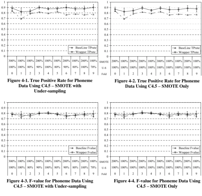
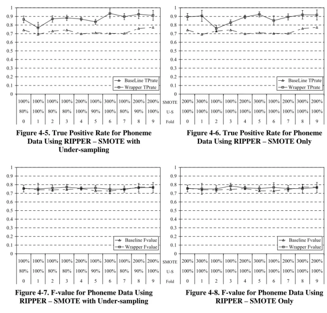
Detailed Results for each fold are provided in the charts in Figure 4-1 to Figure 4-4, where the x-axis is labeled using the percentage of SMOTE and under-sampling performed to obtain the results and the fold number. As indicated earlier, due to the inherent randomness in under-sampling and SMOTEing, to get fair performance measures over the test set, the classifiers were built and evaluated five times using wrapper selected under-sampling and SMOTE percentages. The standard deviation from the average TP-rates and F-values is shown in the charts using standard deviation bars for wrapper results. The baseline results are always constant and do not have standard deviation bars.
SMOTE U-S Fold 0 0.1 0.2 0.3 0.4 0.5 0.6 0.7 0.8 0.9 1 300% 100% 100% 200% 100% 100% 200% 100% 200% 100% 100% 100% 80% 90% 100% 80% 90% 80% 100% 70% 0 1 2 3 4 5 6 7 8 9 BaseLine TPrate Wrapper TPrate 0 0.1 0.2 0.3 0.4 0.5 0.6 0.7 0.8 0.9 1 200% 100% 200% 200% 100% 300% 100% 100% 200% 100% 100% 100% 100% 100% 100% 100% 100% 100% 100% 100% 0 1 2 3 4 5 6 7 8 9 BaseLine TPrate Wrapper TPrate
Figure 4-1. True Positive Rate for Phoneme Data Using C4.5 – SMOTE with
Under-sampling
Figure 4-2. True Positive Rate for Phoneme Data Using C4.5 – SMOTE Only
SMOTE U-S Fold 0 0.1 0.2 0.3 0.4 0.5 0.6 0.7 0.8 0.9 1 300% 100% 100% 200% 100% 100% 200% 100% 200% 100% 100% 100% 80% 90% 100% 80% 90% 80% 100% 70% 0 1 2 3 4 5 6 7 8 9 Baseline Fvalue Wrapper Fvalue 0 0.1 0.2 0.3 0.4 0.5 0.6 0.7 0.8 0.9 1 200% 100% 200% 200% 100% 300% 100% 100% 200% 100% 100% 100% 100% 100% 100% 100% 100% 100% 100% 100% 0 1 2 3 4 5 6 7 8 9 Baseline Fvalue Wrapper Fvalue
Figure 4-3. F-value for Phoneme Data Using C4.5 – SMOTE with Under-sampling
Figure 4-4. F-value for Phoneme Data Using C4.5 – SMOTE Only
From Figure 4-1 and Figure 4-2, it can be seen that the wrapper approach for C4.5 was able to significantly improve TP-rates for the minority class (9.56% and 10.51% increase on average for ‘SMOTE only’ and ‘under-sampling & SMOTE’ respectively) on all 10 test sets, with the wrapper TP-rate using ‘under-sampling & SMOTE’ better than wrapper TP-rate using ‘SMOTE only’. In the case of the ‘SMOTE only’ scenario the wrapper F-values for the minority class were statistically better than the baseline F-values as seen in Table 4-2. Also the F-values on the majority class were statistically worse than the baseline F-values, but the amount of decrease was very small (0.65% and 1.38% on average for ‘SMOTE only’ and ‘under-sampling & SMOTE’ respectively).