Securitization and lending competition

Economics Working Papers (2002–2016) Economics

11-28-2011

Securitization and lending competition

David M. Frankel

Iowa State University, [email protected]

Yu Jin

Iowa State University

Follow this and additional works at:http://lib.dr.iastate.edu/econ_las_workingpapers

Part of theEconomics Commons

This Working Paper is brought to you for free and open access by the Economics at Iowa State University Digital Repository. It has been accepted for inclusion in Economics Working Papers (2002–2016) by an authorized administrator of Iowa State University Digital Repository. For more information, please [email protected].

Recommended Citation

Frankel, David M. and Jin, Yu, "Securitization and lending competition" (2011).Economics Working Papers (2002–2016). 102.

Securitization and lending competition

Abstract

We study the effects of securitization on interbank lending competition when banks see private signals of local applicants' repayment chances. If banks cannot securitize, the outcome is efficient: they lend to their most creditworthy local applicants. With securitization, banks lend also to remote applicants with strong observables in order to lessen the lemons problem they face in selling their securities. This reliance on observables is inefficient, raises the mean default risk, and may lead to a deceptive rise in credit scores.

Keywords

banks, securitization, mortgage backed securities, remote lending, internet lending, distance lending, lending competition, signalling, lemons problem, residential mortgages, default risk, crisis of 2008

Disciplines

I

OWA  

S

TATE  

U

NIVERSITY

Department  of  Economics  

Ames,  Iowa,  50011-­‐1070  

Iowa  State  University  does  not  discriminate  on  the  basis  of  race,  color,  age,  religion,  national  origin,  sexual  orientation,   gender  identity,  genetic  information,  sex,  marital  status,  disability,  or  status  as  a  U.S.  veteran.  Inquiries  can  be  directed   to  the  Director  of  Equal  Opportunity  and  Compliance,  3280  Beardshear  Hall,  (515)  294-­‐7612.  

Securitization and Lending Competition

David M. Frankel, Yu Jin

Working Paper No. 11025 November 2011

Securitization and Lending Competition

David M. Frankel (Iowa State University)

Yu Jin (Iowa State University)

November 28, 2011

Abstract

We study the e¤ects of securitization on interbank lending competition when banks see private signals of local applicants’ repayment chances. If banks cannot securitize, the outcome is e¢ cient: they lend to their most creditworthy local applicants. With securitization, banks lend also to remote applicants with strong observables in order to lessen the lemons problem they face in selling their securities. This reliance on observables is ine¢ cient, raises the mean default risk, and may lead to a deceptive rise in credit scores.

JEL: D82, G14, G21.

Keywords: Banks, Securitization, Mortgage Backed Securities, Remote Lend-ing, Internet LendLend-ing, Distance LendLend-ing, Lending Competition, Asymmetric Information, Signalling, Lemons Problem, Residential Mortgages, Default Risk, Crisis of 2008.

Department of Economics, Iowa State University, Ames, IA 50011, [email protected], [email protected]. We thank seminar participants at Copenhagen, Hebrew U., IDC-Herzliya, Lund,

1

Introduction

Securitization of conventional home mortgages began in 1970 with the founding of the Federal Home Loan Mortgage Corporation.1 The proportion of mortgages held in market-based instruments rose steadily from 20% in 1980 to 68% in 2008.2 _Earlier

evidence indicates that securitization has been growing at least since 1975 (Ja¤ee and Rosen [21, Table 2]).

Remote lending has also grown. Petersen and Rajan [28, Figures I and II] …nd an upwards trend in distances between small …rms and their lenders that began in about 1978 or 1979 and continued through the end of their data in 1992. The mean borrower-lender distance in a sample of small business loans studied by De Young, Glennon, and Nigro [13, pp. 125-6] rose from 5.9 miles in 1984 to 21.5 miles in 2001. Remote lending of residential mortgages also rose from 1992 to 2007 (Loutskina and Strahan [23, p. 1477], discussed below).

We present a tractable theoretical model that links securitization and remote lending. We assume that banks have hard information about all loan applicants but soft information about only local applicants. Without securitization, banks lend only to local applicants because of a winner’s curse. With securitization, in contrast, ignorance is bliss: the less a bank knows about its loans, the less of a lemons problem it faces in selling them.3 This enables banks to compete successfully for some remote applicants.

Our model yields many predictions that are consistent with prior empirical …ndings (section 5.1):

1. Securitization Stimulates Lending. As in Shin [32], securitization leads to

1_{A detailed history of securitization appears in Hill [20].}

2_{The source is unpublished data underlying Figure 3 in Shin [32].}

3_{In a prior empirical paper, Loutskina and Strahan [23] point out that banks may have an}

expanded lending by connecting liquid investors with loan applicants. There is considerable evidence that the securitization boom in the 2000s led to expanded lending (Demyanyk and Van Hemert [12]; Krainer and Laderman [22]; Mian and Su… [24]).

2. Securitization Favors Remote Lending. In our model, banks lend remotely only if they can securitize their loans. Moreover, a bank securitizes all of its remote loans but only some of its local loans. Loutskina and Strahan [23] …nd that as securitization rose, the market share of concentrated lenders - those which originate at least 75% of their mortgages in one MSA - fell from 20% to 4% from 1992 to 2007. Moreover, concentrated lenders retain a higher proportion of their loans. Finally, when they expand to new MSA’s, these lenders are more likely to sell their remote loans than those made in their core MSA’s. 3. Remote Borrowers have Strong Observables but High Conditional

Default Rates. While a bank might lend to a local applicant who has a low credit score in our model, it will not do so for a remote one whose credit score is all it sees. Hence, remote borrowers tend to have stronger observables than local borrowers. (We use “borrower” to refer to an applicant who gets a loan.) On the other hand, since banks lack soft information for remote applicants, they make worse lending decisions: conditional on observables, distant borrowers are more likely to default.4 _{Loutskina and Strahan [23,}

p. 1456] …nd that concentrated lenders (de…ned above) have lower loan losses despite lending to applicants who are riskier in terms of loan to value ratios. Agarwal and Hauswald [1] …nd that applicants with strong observables tend to apply online for loans, while in-person applicants tend to be those with weaker observables but positive estimates of the bank’s soft information about them.

4_{This empirical implication is also present in the prior theoretical model of Hauswald and Marquez}

Moreover, online loans default more than observationally equivalent in-person loans. De Young, Glennon, and Nigro [13] …nd that banks that lend remotely have higher default rates.

4. Securitization Lets Borrowers with Strong Observables Get Cheap Remote Loans. In our model, securitization encourages banks to lend to remote applicants with strong observables. They must o¤er low interest rates to these applicants in order to prevent cream skimming by the applicants’local banks. In contrast, banks can demand high interest rates from quality local applicants whose observables are weak since these applicants cannot get remote loans. This has two empirical implications. First, the securitization boom in the 2000s should have strengthened the (negative) relation between borrower observables and interest rates. Rajan, Seru, and Vig [30] …nd that borrower credit scores and LTV ratios explain just 9% of interest rate variation among loans originated in 1997-2000 but 46% of this variation among loans originated in 2006. A second implication is that remote borrowers pay lower rates.5 Agarwal and Hauswald [1] …nd that internet loans carry lower interest rates than in-person loans. Degryse and Ongena [8] …nd that interest rates decrease with the distance between small …rms and their lenders in Belgium. Mistrulli and Casolaro [25] …nd the same relation among business lines of credit in Italy. 5. Securitization Raises Conditional and Unconditional Default Rates.

Securitization encourages more remote lending in our model. This raises default rates conditional on borrower observables. Securitization also makes lending more pro…table in general, which encourages banks to lower lending standards as in Shin [32]. For both reasons, the unconditional default rate also rises. These predictions are con…rmed by empirical research. Rajan, Seru, and Vig [30] …nd

that conditional default rates rose between 1997-2000 and 2001-6.6 Demyanyk and Van Hemert [12] …nd that conditional and unconditional default rates rose from 2001 to 2007.7

6. Securitized Loans Have Higher Conditional Default Rates than Re-tained Loans. In our model, local banks adopt lower lending standards in local areas that are more pro…table to securitize. Hence, securitized loans have higher default rates than retained loans conditional on observables. Krainer and Laderman [22] …nd that controlling for observables, privately securitized loans default at a higher rate than retained loans. Elul [15] …nds that securi-tized loans perform worse than observationally similar unsecurisecuri-tized loans, and that the e¤ect is strongest in the prime market.

In our model, securitization has mixed e¤ects on social welfare. It raises the sup-ply of funding for worthwhile projects by connecting liquid investors with deserving loan applicants. However, it also leads to an ine¢ cient loan allocation by giving banks an incentive to favor remote applicants with strong observables. For instance, consider two applicants in the same location. One has a high credit score but a negative NPV project. The other has a low credit score but a positive NPV project. A remote bank would favor the …rst applicant since evaluating a project’s NPV re-quires soft information, which it lacks. A local bank may prefer not to fund either applicant because it knows too much about them, which makes their loans di¢ cult to sell. Hence, funds go to the negative-NPV project, which is clearly ine¢ cient.

6_{They control for the loan interest rate, credit score, loan to value ratio, and dummy variables}

for adjustable rates, prepayment penalties, and whether the lender lacked documentation of the borrower’s income or assets.

7_{Their controls include the loan interest rate, borrower credit score, loan to value ratio, debt to}

income ratio, local changes in house prices and unemployment since origination, and dummies for prepayment penalties, owner-occupier status, and low documentation.

We treat securitization as an exogenous innovation that encourages remote lend-ing. If instead securitization were initially possible and an exogenous barrier to re-mote lending were then lifted, our model would also predict a simultaneous increase in both remote lending and securitization.8 _{In practice, legal barriers to interstate}

banking fell gradually starting in Maine in 1978 and ending with the federal govern-ment’s passage of the Interstate Banking and Branching E¢ ciency Act of 1994, which abolished all remaining restrictions (Loutskina and Strahan [23, pp. 1451-2]). Since securitization was invented earlier, these barriers may have fallen partly in response to pressure from large banks who were eager to increase their securitization pro…ts. Alternatively, their fall may have been due to an exogenous change in regulatory philosophy. This is an interesting topic for future empirical research.

The rest of the paper is as follows. The model is presented in section 2. Section 3 analyzes a base case without securitization, while the full model is studied in section 4. The model’s predictions are discussed and illustrated in section 5. Section 6 reviews related theoretical literature, while conclusions appear in section 7.

2

The Model

A country consist of two ex ante identical regions,A and B, each containing a single bank. We will refer to the bank in region A (B) as bank a (respectively, b). Each region R_{2 f}A; B_g consists of a continuum of locations` <sub>2</sub>[0;1]. In each location `

there is a continuum of agents. All participants are risk-neutral.

Each agent has a project that requires one unit of capital and pays a …xed gross return of >1 if it succeeds and zero otherwise. The project’s success probability

8_{Since we assume banks lack private information about their remote loans and have a lower}

discount factor than investors, banks securitize all of their remote loans. Since in our model -they securitize only some of their local loans, removing a barrier to remote lending would raise the proportion of loans that are securitized.

is the product of the agent’s unknown type ₂ (0;1) and a macroeconomic shock

SR

` 2 (0;1) to the agent’s location ` in the region R in which she lives. Project

outcomes, conditional on these success probabilities, are independent.9

There are four periods, t = 1;2;3;4. Period 1 is the lending stage. The banks see signals of each agent’s type and then make competing loan o¤ers to the agents. This stage determines which agents borrow from which banks, and at what interest rates. Period 2 is the security design stage. Each bank decides which loans to securitize and what liquidating dividend to pay as a function of the returns of these loans. Period 3 is the signalling stage. The bank in each region R …rst sees signals of its local macroeconomic shocks SR

` . Each bank then chooses how many shares of

its security to sell to investors. Period 4 is the settlement stage: project returns are realized, successful borrowers repay their loans, and each bank pays a liquidating dividend to holders of its security.

The local shock SR

` has the form

S<sub>`</sub>R = K X k=1 R k` R k: (1)

For each k, R_{k 2}(0;1) is a random variable that is realized after the security is sold and Rk` 2 [0;1] is a constant satisfying

PK k=1 R k` 1.10 We refer to R k as the

kth local factor in region R and to R

k` as location `’s loading on this factor. For

instance, each factor may represent an industry and the factor loading may be the share of a location’s workforce that is employed in the industry.11 _{In each region R,}

the distribution of the factor loading vector Rk` K

k=1 across locations` 2[0;1]has no

atoms.12

9_{That is, a project’s success probability is S}R

` regardless of the outcomes of other projects.

10_{One can include a constant term in equation (1) by assuming that one of the factors is a constant.} 11_{Factor dependence within and across regions is permitted, as detailed below in section 2.1.3.} 12_{That is, there is no factor loading vector that receives a strictly positive probability weight.}

At the beginning of period 1, both banks see a public signal spub 2(0;1) of type

of each agent. Simultaneously, the agent’s local bank also sees a private signal

spriv 2 (0;1) of .13 The joint population distribution of the type , signals spub

and spriv, and location` is given by a known distribution function F and associated

continuous density functionf on the domain (0;1)3 [0;1].

The assumption thatF is region-independent is purely for notational convenience. It could be replaced by region-speci…c distribution functions FA _{and F}B _{with no}

change in the results, except for the proliferation of region superscripts throughout the paper. The same is true of all distributions derived from F. In particular, we will also useF to denote the marginal and conditional distribution functions of these variables or subsets of them; for instance, F ( _jspriv; spub; `) denotes the conditional

distribution of given spriv, spub, and `. The corresponding densities are written

with “f” in place of “F”, and we assume that all such densities are continuous. We assume that an increase in the public signal - or in the private signalconditional

on the public signal - raises the conditional distribution of in a …rst-order stochastic dominance sense. This is formalized in the following two assumptions. The …rst says that an increase in the public signal weakly lowers the probability of observing a type below any given threshold, and strictly lowers the average of these probabilities across thresholds. Moreover, this e¤ect is bounded above. The second property is like the …rst but relates to the e¤ect of the private signal on the distribution of types conditional on the public signal. (In both cases, we also condition this distribution on the location`.)

Public Signal Monotonicity For any signal spub 2 (0;1) and location ` 2 [0;1],

there are integrable functions : (0;1) _{! <}+, such that the integral

R1

=0 ( )d is strictly positive and for each 2(0;1), the derivative

@F( jsp u b;`)

@sp u b exists and lies between ( ) and ( ), inclusive.

13_{The outcome of the model will not depend on what the applicant knows about her own type, as}

Private Signal Monotonicity For any signals spub; spriv 2 (0;1) and location ` 2

[0;1], there are integrable functions : (0;1) _{! <}+ such that the

in-tegral R1₌₀ ( )d is strictly positive and for each ₂ (0;1), the derivative

@F( jsp riv;sp u b;`)

@sp riv exists and lies between ( ) and ( ), inclusive.

Let =E[ _jspub; `]

d

= (spubj`)denote an agent’s expected type given her public

signal and location; let = 1E[ _jspub; spriv; `]

d

= (sprivjspub; `) denote the

propor-tional change in this expectation that results from learning her local bank’s private signal.14 By the Law of Iterated Expectations, E( _j ; `) is identically equal to one. Henceforth, we will work directly with and , which we refer to respectively as the agent’s credit score and private type. The following result states that (a) the credit score is strictly increasing in the public signal and (b) conditional on the public signal, the private type is strictly increasing in the private signal. Moreover, both rates of increase are bounded.

Claim 1 The functions (spubj`) and (sprivjspub; `)have slopes (with respect to spub

and spriv, respectively) that are strictly positive and …nite.

Claim 1 has the following useful implication. Let us say the pair ( ; `) isfeasible

if the location`is in[0;1]and the credit score lies strictly betweensup_s

p u b (spubj`) and infsp u b (spubj`). All feasible pairs have a …nite, strictly positive probability density:

Claim 2 The pair ( ; `) is distributed according to a …nite densityg which is strictly positive on the set of feasible pairs ( ; `).

Let the distribution function of ( ; `) be denoted G( ; ). Let the conditional distribution function of the private type given the credit score and location ` be

denotedH( _j ; `). With probability one, the support ofH(<sub>j</sub> ; `)has a …nite supre-mum `.15 We assume thatH is not too concave, and its concavity is nondecreasing

in :

No Cream Skimming Let H0 _{and H}00 _{denote the …rst and second derivatives of}

H( _j ; `)with respect to . For all feasible pairs ( ; `) and for all in the interior of the support of H(_j ; `), (a) these derivatives exist and (b) H00 _=H0

is greater than 1 and is weakly increasing in .

This property will imply that if banka(for instance) lends to some agents with credit score in location ` in region B, then bank a prefers to charge an interest rate that is low enough to deter bank b from lending to any agents in this group. Hence, in equilibrium bankb does not “cream skim”: lend to agents with high private types but not to all agents. This fact allows us to solve analytically for the interest rates that the banks charge for every credit score, location, and region. It is consistent with the observation of Agarwal and Hauswald [1] that internet lenders charge low rates partly in order to prevent cream skimming:

Arm’s-length debt is less readily available but carries lower rates be-cause competition among symmetrically informed banks, which rely on public information, not only drive down its price but also restrict access to credit to minimize adverse selection. [Agarwal and Hauswald [1, p. 2]] The following result shows that No Cream Skimming is equivalent to a particular assumption on the primitives of the model.

Claim 3 Let F0 _{and F}00 _{denote the …rst and second derivatives of F (s}

privjspub; `)

with respect to spriv. Let 0 and 00 denote the …rst and second derivatives of =

15_{Since 1,}

` is no greater than 1= . Since >0, =E( jspub; `) is strictly positive for

any spub that occurs with positive probability. Hence,1= is …nite with probability one, so ` is

(sprivjspub; `) with respect tospriv. Assume these derivatives exist. Then No Cream

Skimming holds if and only if, for all spriv,spub, and`, F

00

F0 0 00

[ 0]2 is greater than 1

and is weakly increasing in spriv.

The following property states that for any given public signal, one can …nd private signals that are strong enough that make an agent at least as appealing as any other agent. For instance, if an agent with several loan delinquencies (the public signal) has just inherited a large enough sum of money (the private signal), a bank can ignore her weak credit history.

Limit Irrelevance For any public signal spub, location `, and " > 0, there exists a

private signal spriv for which E[ jspub; spriv; `]>1 ".

This will imply that a remote bank lends to applicants whose credit scores exceed a location-dependent threshold.16 Indeed, Agarwal and Hauswald [1] …nd that the chance that a bank will approve an online loan is increasing in both the applicant’s public credit quality and the bank’s internal assessment, but the latter’s e¤ect is very small. Limit Irrelevance permits the depiction of our results using simple two-dimensional diagrams. We also consider what happens in the absence of this as-sumption.

We now produce an example that satis…es all of the above assumptions. Suppose that spriv, spub, and` are independent and each is uniformly distributed on the unit

interval.17 This implies that F (sprivjspub; `) =spriv, so F00 = 0. Let the conditional

distribution of given the two signals and location beF ( _jspriv; spub; `) =

m

1 m where

m= 1 (1 spriv) (1 spub). The mean of this distribution,E( jspriv; spub; `), equals

16_{Without Limit Irrelevance, a bank may o¤er loans in a given remote location to applicants with}

credit score 0 _{but not to those whose credit scores are} 00_> 0_.

17_{This refers to the closed unit interval in the case of` and the open interval in the case ofs} priv

m. Hence, (sprivjspub; `) = E( <sub>j</sub>spriv; spub; `) E( _jspub; `) = 1 (1 spriv) (1 spub) 1 1 sp u b 2 ;

so 00 = 0as well. No Cream Skimming then follows from Claim 3. Limit Irrelevance holds since limsp riv!1E( jspriv; spub; `) = 1. Since

m

m 1 is strictly increasing in m,

which is strictly increasing inspriv, Private Signal Monotonicity holds. Public Signal

Monotonicity holds since F( _jspub; `) =

R1

sp riv=0F ( jspriv; spub; `)dspriv.

2.1

Timing

We now describe each period in greater detail.

2.1.1 Period 1: Lending Stage

In period 1, the banks o¤er loans …rst to remote agents and then to local agents. That is, banksa and b …rst make simultaneous and public loan o¤ers to agents who live in regions B and A, respectively. These o¤ers can depend on an agent’s credit score and location `, which are all the banks know. The banks then make simultaneous and public counter-o¤ers to agents who live in regionsA and B, respectively. These o¤ers can depend not only on and `, but also on an applicant’s private type and her o¤er (if any) from her remote bank. Each agent then chooses which, if any, o¤er to accept. As the banks are perfect substitutes from an agent’s point of view, an agent will choose the bank that o¤ers her the lowest gross interest rate as long as it does not exceed the project return .

Let xB

` equal one if bank a chooses to compete for agents with credit score in

location`in regionRand zero otherwise. LetrB

`be the gross interest rate that bank

a o¤ers if xB

` = 1. We assume this rate does not exceed the gross project return ,

since o¤ering a rate above is equivalent to not making an o¤er. If the agent did not receive an o¤er from banka, then she is willing to pay bankb her gross project return

. Thus, with the convention that rB

rB_` equals the willingness to pay of any agent. We assume there is an in…nitesimal chance that the secondary loan market will be disrupted, forcing the bank to hold all of its loans to maturity. Since only bank b observes an agent’s private type , this implies that a threshold strategy is optimal: bankb will bidrB

` (and win) as long as

an agent’s private type exceeds a threshold B

` of bank b’s choosing. Otherwise,

bankb will not bid.

The banks swap roles with respect to agents who live in region A. Let xA ` equal

one if bank b chooses to compete for agents in region A with credit score and location `, and zero otherwise. Let rA

` equal bank b’s bid in period 1 ifx ` = 1;

setrA

` = otherwise. In period 2, bank a responds by choosing thresholds A` such

that it will lend an agent in region A at interest rate rA

` if and only if the agent’s

private type exceeds A

`.

Let CB

a and XaB be the capital cost and realized value, respectively, of bank a’s

loans to region B: C_aB = Z 1 `=0 Z 1 =0 xB<sub>`</sub>H B<sub>`j</sub> ; ` dG( ; `) X<sub>a</sub>B = Z 1 `=0 Z 1 =0 xB_{`</sub>rB<sub>`} " S<sub>`</sub>B Z B ` =0 dH( _j ; `) # dG( ; `)

Thus,C_aB is the integral, over all credit scores and locations` in region B in which the bank competes (i.e., for which xB

` = 1), of the measure H B`j ; ` of borrowers

to whom bank a lends. Likewise, X_aB is the integral, over all credit scores and locations ` in regionB in which bank a competes, of the interest rate rB

` charged to

these borrowers times their mean probability of repayment (the expression in square brackets).

banka’s loans to regionA: C_aA = Z 1 `=0 Z 1 =0 1 H A<sub>`j</sub> ; ` dG( ; `) X_aA = Z 1 `=0 Z 1 =0 rA<sub>`</sub> " S<sub>`</sub>A Z ` = A<sub>`</sub> dH( <sub>j</sub> ; `) # dG( ; `)

The di¤erence betweenC_aAand C_aB re‡ects the fact that banka lends to borrowers in region A whose private types exceed bank a’s minimum threshold A

`, while it lends

to borrowers in regionB if and only if (1) it chooses to compete for them (i.e., only if

xB

` = 1) and (2) their private types are below bank b’s minimum threshold B`. This

also explains the di¤erence between X_aA and X_aB.

2.1.2 Period 2: Security Design Stage

In period 2, each bank designs one security. The number of shares of each security is normalized to one. We describe this process from the point of view of bank a; bank b’s problem is analogous. First, bank a decides what portion of the loans of each identi…able group of borrowers to securitize: to include in the pool of assets that underlie its security. Bank a does not know the private types of its borrowers in region B. Hence, for any given credit score and location `, it must securitize the same proportion of loans to each type ₂ 0; B

` of borrower in region B. Let

this proportion bepB `.

As for region A, since a borrower’s private type is observed by bank a but not by the market, banka will securitize a loan if and only if the borrower’s private type

is less than some threshold A

`, which must be at least as high as the minimum

private type A

` of borrowers in regionAto whom the bank lends. The realized value

of banka’s securitized loans is Ya=YaA+YaB where

Y_aA= Z 1 `=0 Z 1 =0 rA<sub>`</sub> " S<sub>`</sub>A Z A ` = A ` dH( <sub>j</sub> ; `) # dG( ; `) (2)

is the realized value of the bank’s securitized local loans and Y_aB = Z 1 `=0 Z 1 =0 pB<sub>`</sub>xB_{`</sub>rB<sub>`} " S<sub>`</sub>B Z B ` =0 dH( _j ; `) # dG( ; `) (3)

is the realized value of the bank’s securitized remote loans. One obtains Y_aA from

XA

a by replacing the supremum ` of private types in XaA with the upper bound A

` on private types who are securitized. Similarly, one obtains Y B

a from XaB by

multiplying the integrand of the outer double integral in XB

a by the proportionpB` of

loans that are securitized.

After choosing which loans to securitize, each bank i=a; bchooses a function '_i

which determines the ultimate payment per share made by the bank to a holder of its security as a function of the realized loan repayments Yi of bank i’s securitized

borrowers. We call '_i(Yi) the payout of the security. As in DeMarzo and Du¢ e

[10], we assume that'_i is a nondecreasing function and that both the bank and the market have limited liability: '_i(y)₂[0; y] for all y 0.

There is symmetric information at the security design stage. Why? Let R(i)

denote the region in which banki_{2 f}a; b_gis located. While the thresholds R_`(i) and

R(i)

` are the private information of bank i=a; b, the market can infer the values YiA

and Y_iB of bank i’s securitized local and remote loans that result from each pair of factor vectors A; B in the following way. First, we assume the market observes the measure 1 H R<sub>`</sub>(i)<sub>j</sub> ; ` of bank i’s local borrowers for each credit score and location `, as well as the proportion H

R(i)

` j ;` H

R(i)

` j ;`

1 H R<sub>`</sub>(i)j ;` of these borrowers

whom bank i securitizes. From these quantities, the market can infer the values

H R<sub>`</sub>(i)<sub>j</sub> ; ` andH R<sub>`</sub>(i)<sub>j</sub> ; ` of the distribution functionH at the two thresholds. We also assume that for each regionR, the market observes the interest ratesrR_`, the lending choices xR

`, and the remote securitization proportions pR`. The market can

then use equations (2) and (3), or the corresponding equations for bankb, to compute

YA

i and YiB for any factor vectors

2.1.3 Period 3: Signalling Stage

In period 3, the banks and investors …rst see a common public signal _{2 <}M_{, with}

unconditional distribution function . Each bankithen sees a private signalui

2 <N +

of its local factor vector R(i) ₂ (0;1)K. The local factor vector R(i) and the local signal ui _{are drawn from a joint density} R(i)_{; u}i

j , which can depend on the

public signal as indicated by the notation. However, conditional on the public information , A; ua _and B_{; u}b _{are independent: the realization of} A_{; u}a

adds no information about the distribution of B; ub _{and vice-versa. This is a}

‡exible yet tractable way to permit common or correlated shocks to the two regions. Let the distribution function of the private signal ui _{conditional on the public}

signal be (ui

j ). We assume that for all public signals , private signalsui _close

to the zero vector are observed with strictly positive probability:

inf ui _{2 <}N₊ : ui_j >0 = 0:

Let R(i)_jui_{; be the conditional distribution of the factor vector} R(i)

given the private signal ui _{and the public signal . A higher private signal u}i _{raises this}

distribution in the sense of …rst order stochastic dominance: if u0 _u00_{, then for all}

, ( _ju0_{; ) ( ju}00_{; ). This implies that for any public signal , the worst news}

bank i can get about its security payout '_i(Yi) occurs when its private signal ui is

zero. Finally, we assume that the conditional distribution R(i)_jui_{; is mutually}

absolutely continuous with respect to the signals (ui_{; ).}18

The assumption that the density and distributions and are region-independent is for notational convenience. They could be replaced by R_, R_{, and} R _{with no}

change in the results, except for the proliferation of regional superscripts throughout the paper.

After seeing their signals, the banks choose quantities of their securities to sell.

18_{This means that the set of realizations of the factor vector} R(i) _{that can occur with positive}

Bank i’s quantity is denoted qi 2 [0;1]. The market (which also sees the public

signal ) uses Bayes’s rule to assign a price pi =E['i(Yi)jqa; qb; ] to the security of

banki=a; b. This is a nonstandard signalling game since the market rationally uses information about bank i’s quantity qi to infer information about banki’s signal ui,

which may be relevant to the value of bankj’s security (as it may include some loans to borrowers in bank i’s region).

2.1.4 Period 4: Settlement Stage

In period 4, each borrower repays her loan if and only if her project succeeds. These repayments determine the value Yi of bank i’s loan portfolio. Bank i then pays the

liquidating dividend '_i(Yi)to its investors. While periods 1 through 3 occur at the

same point of real time, there is a unit of delay between periods 3 and 4.

2.2

Payo¤s

A borrower who pays interest rate r gets r if her project succeeds and zero otherwise. The banks are liquidity constrained: the discount factor of security buyers, which we normalize to one, exceeds the discount factor of the banks, which is denoted 2(0;1).19 _{The two banks have the same cost of capital, which is normalized to one.}

In particular, suppose a bank lends c1 units of capital in period 1 to borrowers who

later repay the bankc4 in period 4. Assume, moreover, that investors pay the bank

c3 in period 3 in return for a security that obligates the bank to pay the investors

c0₄ in period 4. Then the payo¤ of investors in the bank’s security is c0₄ c3, while

the bank’s payo¤ equals c3 c1+ (c4 c04): its securitization proceeds c3, less its

capital cost c1, plus its discounted loan repayments c4, less its discounted payment

19_{This assumption, common in the prior literature, is thought to capture the typical reason cited}

for why banks sell loans: the availability of attractive alternative investments together with the existence of regulatory capital ratios (e.g., Gorton and Haubrich [16, §III.B]).

c0

4 to holders of its security. We assume the investors have at least2 in capital to

invest.20

2.3

Summary

We now brie‡y summarize the key features of the model. We focus on region B; analogous choices are made simultaneously in regionAwith the banks’roles swapped. Consider the group of agents with a given credit score and location`. In period 1, banka either o¤ers each such agent a loan at the common interest raterB

` 2[0; ]or

refrains from competing (whence we setrB

` = ). Bankb then lends, at the interest

rate rB

`, to those agents in the group whose private types exceed a threshold B` of

bankb’s choosing. Agents with lower private types accept a’s o¤er, if any. In period 2, bank a chooses a proportion pB

` 2 [0;1] of its loans to the group

to securitize. Bank b securitizes its loans to group members whose private types fall below a threshold B

` of bank b’s choosing Each bank i also speci…es a payout

function '_i.

In period 3, each bank i=a; b sees a signalui _{of its local factor vector and then}

chooses a quantity qi 2[0;1] of shares to sell. The market rationally assigns a price

pi to bank i’s security using Bayes’s rule. In period 4, project returns are realized

and successful borrowers repay their loans. Each banki then pays '_i(Yi) per share

to its security holders, where Yi equals the repayments of bank i’s securitized loans.

3

Base Model: No Securitization

We …rst analyze a base model without securitization: banks must hold all of their loans to maturity. Bank a’s payo¤ in the base model is simply its discounted loan repayments less its cost of lent capital: E XA

a +XaB CaA CaB. Bankb’s payo¤

20_{Since each region has a unit measure of loan applicants, each with a project that returns if it}

is analogous. In particular, if a bank lends, at a gross interest rate r, to a borrower with credit score and private type living in location ` in region R <sub>2 f</sub>A; B<sub>g</sub>, its expected pro…t is r E S<sub>`</sub>R 1: the discounted interest payment r times the

probability E SR

` of project success, less the unitary cost of capital.

In the base model, banks lend only to local agents and extract the full surplus. This is due to the winner’s curse: the banks have the same expected payo¤ from lending to a given agent, but the agent’s local bank has superior information about this payo¤. Since, by assumption, the local bank makes the second o¤er, it will slightly underbid the remote bank on pro…table loans but refrain from bidding on unpro…table ones. Knowing this, a bank will not make any o¤ers to agents who are not in its region.

Claim 4 Without the option of securitization, each bank lends only to agents who reside in its own region. Moreover, each borrower’s payo¤ is zero: the gross interest rate on every loan equals the gross project return . An agent gets a loan if and only if her discounted expected gross project return, E SR

` , exceeds the bank’s

unitary cost of capital.

Without securitization, an agent gets a loan if and only her expected project return exceeds a common threshold. Hence, the allocation of capital to projects is e¢ cient: one agent receives a loan while another does not if and only if the …rst has a higher expected project return than the second. This e¢ ciency property will not hold with securitization, since a bank may prefer not to lend to a creditworthy agent whom it knows well. Intuitively, the bank’s private information about this borrower’s repayment probability worsens the lemons problem the bank faces in selling its security.

Our conclusion that all lending is local and the loan allocation is e¢ cient relies on our assumption that the remote bank makes the …rst o¤er, followed by the local bank. However, Sharpe [31] obtains the same result with the reverse timing. He assumes

that the remote bank sees not the local bank’s o¤er but rather its o¤er function: the function from the local bank’s signal to its interest rate. If, in addition, the remote bank has no private information about the applicant, then the local bank always posts an o¤er function that is low enough to make it unpro…table for the remote bank to compete because of a winner’s curse (Sharpe [31, Proposition 2, p. 1078]).

4

Full Model

We now turn to the full model, with securitization. We …rst show that the signalling subgame has a unique separating equilibrium. We then derive formulas for a bank’s bene…t of securitizing a given loan and of lending to a given borrower when securi-tization is an option. Finally, we show that any equilibrium of the full model must have a certain intuitive form. We then turn to several computed examples.

4.0.1 The Signalling Subgame

Let i(ui; uj; ) = E['i(Yi)jui; uj; ] be the expected payout of the security of bank

i_{2 f}a; b_g, conditional on the signals. (“j”refers to the other bank.) Letpi(qi; qj; )

be the price o¤ered by the market per unit of bank i’s security as a function of the quantities of shares sold by the two banks and the public signal. Bank i’s expected securitization pro…ts i_(ui_{; q}

i; ), conditional on its signalui and quantity qi and the

public signal equal the expectation (over all opposing signal vectors uj_{) of banki’s}

gross revenueqipi(qi; qj(uj); )from sellingqi units of the security less its discounted

expected payment to the buyers, qi i(ui; uj; ): i ui; qi; = Z uj_2<N + qi pi qi; qj uj ; i u i ; uj; d uj :

De…nition 5 A Bayes-Nash equilibrium of this game is a pair (qa; qb) of measurable

1. for i=a; b, qi(ui; )2arg maxq i(ui; q; ) almost surely;

2. for i = a; b, pi(qi(ui); qj(uj); ) = E[ i(ui; uj; )jqi(ui); qj(uj); ] almost

surely;

The equilibrium is separating if, in addition,

3. for i=a; b, pi(qi(ui); qj(uj); ) = i(ui; uj; ) almost surely.

We restrict to separating equilibria, which satisfy conditions 1 and 3 above. This restriction uniquely determines the banks’ behavior and pro…ts. Let bi(ui; ) =

R uj_2<N + i(u i_{; u}j_{; )d (u}j j )and i_(ui_{; ) =} i_(ui_{; q} i(ui; ); ) be banki’s expected

security payout and securitization pro…ts, both conditioned only on bank i’s signal

ui _{and the public signal . (In general,} i_(ui_{; ) may depend on the equilibrium.)}

The following characterization extends the result of DeMarzo and Du¢ e [10, eq. (4), p. 79, and Prop. 10, p. 88], which assumes a single bank, to the case of two banks.21

Claim 6 The above double signalling game has a unique separating equilibrium. In it, bank i’s expected securitization pro…ts conditional on its signal ui and the public signal are i_(ui_{; ) = (1 )}b

i(0; )

1

1 b

i(ui; ) 1 . Moreover, each bank i’s

optimal security design is debt: '_i(Yi) = minfmi; Yig for some mi 2 <+.

4.0.2 The Bene…ts of Securitization

Consider either banki_{2 f}a; b_g. By Claim 6, the realized payout of the bank’s security ismin_fmi; Yigwhere Yi =YiA+YiB is the realized value of bank i’s securitized loans

and mi is the face value (promised repayment) of the security. Consequently, the

expected payoutbi(ui; )of banki’s security given its signalui and the public signal

is E[min_fmi; Yig jui; ]. Bank i’s expected payo¤ i is the discounted expected

return of its loans, less its cost of lending, plus its net securitization pro…ts. By

Claim 6, i = E XiA+X B i C A i C B i + (1 )E b_i(0; )11 b_i(ui_{; )}1 !

In order to understand bank i’s incentives to lend to a given agent, one must …rst consider its bene…t from securitizing the agent’s loan. To study this, we hold …xed the bank’s loan portfolio, and consider the e¤ect of adding a single in…nitesimal loan to the bank’s security.

Suppose the recipient of this loan has credit score and private type , and lives in location ` in region R _{2 f}A; B_g.22 _{Let r be the gross interest rate that}

she must pay if her project succeeds, which occurs with probability SR

` . By

Claim 6, and the law of iterated expectations, banki’s expected securitization pro…ts are(1 )EhE b_i(0; )11 b

i(ui; ) 1

i

, where the outer expectation is taken with respect to the public signal and the inner conditional expectation is taken with respect to the private signal ui_{. The e¤ect, on the bank’s pro…ts}

i, of adding the

borrower to the bank’s security is thus

i = (1 )E " E bi(0; ) 1 1 b_i(ui_{; )}1 b_i(0; ) b_i(0; ) b_i(ui_{; )} b_i(ui_{; )} ! !# : (4)

where for any quantity Q, Qdenotes the change in Q that results from adding the loan.

The terms bi(0; ) and bi(ui; ) measure the loan’s e¤ect on the expected

gross returnb_i(ui_{; ) =E[min}

fmi; Yig jui; ]of the security in two cases: when the

bank’s private signal is zero, and when it takes a generic value ui. In particular, by Claim 6, adding the loan is bene…cial insofar as it raises the gross return of the security in the worst case, or lowers it in the generic case. Since higher signals ui

entail higher values of Yi in a …rst order stochastic dominance sense, bi(0; )cannot

22_{We assume that the market knows the private type since it can infer the set of private types}

exceed bi(ui; ). Thus, roughly speaking, loans that shrink (raise) the gap between

b_i(ui_{; ) and} b

i(0; ) must raise (lower) the bank’s securitization pro…ts.

The term bi(ui; ) = E[ minfmi; Yigjui; ] measures the e¤ect of the loan

on the bank’s expected payment to its security holders, conditional on the signals ui

and . This e¤ect occurs entirely through the loan’s impact on the realized value

Yi of the bank’s securitized loans. First, the security defaults when its face value

mi exceeds the value Yi of the underlying loans. In this event, the loan raises the

security payout by Yi. Second, the loan lowers the chance of default by raising the

realized value of the loan portfolioYiwhen this value lies slightly below the face value

of the security, mi. This e¤ect is approximately equal to the product of two terms:

the loss mi Yi from default and the probability thatYi is slightly below mi. Since

both terms are close to zero, this second e¤ect is zero to …rst order. Hence, the only e¤ect is the …rst:

b_i ui; =E 1 (mi > Yi) Yijui; ; (5)

where1 (mi > Yi)equals one ifmi > Yi (if the security defaults) and zero otherwise.

Finally, by (1), the increase in the value Yi of the underlying assets from adding

the borrower is a weighted sum of the macroeconomic factors Rk that a¤ect regionR:

Yi =r S`R=r K X k=1 R k` R k: (6)

Substituting (5) and (6) into (4) and using Claim 6, we …nd that the e¤ect of securi-tizing the additional borrower on the bank’s payo¤ is

i =r Ri`; (7) where R i` =E R i`( ) ; (8) R i`( ) =E i _ui_; j K X k=1 R k` R0 ik ( ) R ik( ) ;

R0 ik ( ) =E E 1 (mi > Yi) Rk ui = 0; b_i(0; ) ! , and R ik( ) =E i_(ui_{; )} E( i_(ui_{; )j )} E 1 (mi > Yi) Rk ui; b_i(ui_{; )} ! :

By (7), pro…ts from securitizing the loan are the product of four terms. The …rst is the gross interest rater: ceteris paribus, it is more pro…table to securitize loans that have a higher face value. The second is : it is more pro…table to securitize the loans of borrowers with higher credit scores. The third is : borrowers with high private types are also more pro…table. The …nal term is R

i` which, by construction, must

equal the change in securitization pro…ts from adding a loan for which the product

r of the …rst three terms equals one.

By (8), R

i` is the expectation, over all public signals , of the change Ri`( ) in

securitization pro…ts from adding a loan for which the productr = 1and the public

signal is . R

i`( ), in turn, is the product of the bank’s conditional (on the public

signal ) expected securitization pro…ts E[ i_(ui_{; )}

j ]and the sum, over all factors

k, of the borrower’s factor loading R

k` times the scaled di¤erence between two terms: R0

ik ( ) and Rik( ).

The term R0

ik ( ) is the proportional increase in the lowest conditional expected

security payout, bi(0; ), that results from increasing the value Yi of the security’s

underlying assets by one dollar with probability R_k.23 _Thus, PK k=1

R

k` Rik0( )

cap-tures the additional loan’s proportional e¤ect on thisworst-case security payout that is due to the loadings R

k` of the borrower’s repayment probability on various

macro-economic factors Rk. Likewise, Rik( )is a weighted average over signal vectorsui of

the proportional increase in the conditional expected security payout b_i(ui_{; ) that}

results from increasing the value Yi of the security’s underlying assets by one dollar

with probability R_k. Thus, PK_k=1 R

k` Rik( ) captures the proportional e¤ect of the

23_{In the numerator of} R0

ik (s), the default indicator variable1 (mi> Yi) is present because the

additional loan on thisweighted averagesecurity payout that results from the loadings of the borrower’s repayment probability on the various macroeconomic factors that a¤ect region R.

By Claim 6, for any public signal , the bank’s securitization pro…ts are increas-ing in the expected security payo¤ conditional on the worst signal vector ui _{= 0 and}

decreasing in the expected security payo¤ for a generic signal vectorui_{. For this}

rea-son, R0

ik ( )enters positively in Ri`( ) while Rik( ) enters negatively. The discount

factor multiplying R

ik( ) captures the bank’s preference for liquidity: the lower

is , the stronger are the bank’s liquidity needs, and thus the more likely it is that securitizing the additional loan will be worthwhile.

The above results allow us to derive a concise expression for the total expected gross return to bank i _{2 f}a; b_g from lending to an agent with credit score and private type who lives in location` in regionR_{2 f}A; B_g, when securitization is an option. This expected return has two parts. The …rst is the expected discounted loan repayment by the borrower, r E SR

` : the discounted interest rate r times

the probability E SR

` that the loan will be repayed. The second is the value of

the bank’s option to securitize the loan. By (7), bank i earns an additional r R i`

from securitizing the agent’s loan, which it will do if and only if R

i` > 0. For any

real number c, let c+ _{denote the positive part of c: c}+ _{= max}

f0; c_g. The value of the securitization option isr R

i` +

, so the bank’s gross return from lending to the borrower is

r h E S_{`</sub>R + R<sub>i`} +i: (9)

Bank i knows the private type of the borrower only if she lives in the bank’s home region. This is a disadvantage of remote lending. However, there is also a potential advantage: the bank does not have private information about remote shocks. Hence, it faces a lemons problem in reselling local loans but not remote loans. In addition, the bank has a preference for liquidity: <1. For the last two

reasons, it is always pro…table to securitize a remote loan:

Claim 7 Let i ₆= j be the two banks. In any equilibrium, it is pro…table for bank i

to securitize all of its remote loans: R_i`(j) >0.

4.0.3 Main Results

We present results for region B. Identical results hold for region A upon replacing “a” with “b” and vice versa. Let rB

` denote the deterring rate: the interest rate,

o¤ered by bank a, that makes bank b just willing not to lend to the agent with the highest private type (for whom = `) among those with credit score living in

location` in regionB. By equation (9), bankb’s gross expected return from lending to this borrower at the interest raterisr `

h

E SB

` + Bb`

+i

. Setting this equal to the bank’s unitary cost of capital and solving for r, we obtain the deterring rate:

rB<sub>`</sub> = ( `) 1

h

E S_{`</sub>B + B<sub>b`} +i 1 >0: (10) Now consider the set of borrowers with credit score in location ` in region B. No Cream Skimming implies that if bankacompetes for these borrowers, it prefers to lend to all of them: to prevent bankb from skimming the best (highest- ) borrowers in the group. This requires banka to bid an interest rate that is no higher than the deterring rate rB<sub>`</sub> . In addition, bank a cannot charge more than the gross project return , which is the most any borrower will pay. On the other hand, any interest rate below the lesser of and rB

` permits bank a to capture all of the borrowers in

this group. Hence, if bank a competes for these borrowers, it will o¤er the interest rate rB

` = min ; rB` . By equation (9), Claim 7, and the fact that E( j ; `) = 1,

banka’s pro…ts from lending a unit of capital to this group are

B

` = min ; rB` E S`B + Ba` 1: (11)

Theorem 8 Consider the group of agents with credit score in location ` in region

B.

1. Suppose B` <0. In this case,

(a) bank a does not compete for this group;

(b) if bankb’s estimate of an agent’s type exceeds h E SB

` + Bb`

+i 1

, bankb o¤ers her a loan at an interest rate equal to the gross project return

, and the agent accepts.24 _{Else bank b does not o¤er the agent a loan.}

Bank b securitizes all borrowers in this group to whom it lends if B b` >0

and none of them if B b` <0.

2. Suppose B

` >0. In this case,

(a) bank a o¤ers to lend to each agent in the group at the common interest raterB

` = min ; rB` ;

(b) bank b makes no o¤ers to this group;

(c) all agents in the group accept bank a’s o¤er; and (d) bank a securitizes all of them.

Consider the set of borrowers in a given location ` in region B. Theorem 8 characterizes the outcome, in the loan market, of borrowers with agiven credit score in this set. It does not show how this outcome varies by the credit score . We now turn to this important question.

The key di¢ culty is that bank a’s pro…t B

` from lending is not necessarily

monotonic in the agent’s credit score . This pro…t is increasing in the deterring rate

rB

` (equation (11)) which, in turn, is decreasing in the supremum ` of the agent’s

supremum ` varies with the credit score . Limit Irrelevance pins this down in a

particular way: ` equals the inverse of the credit score .25 By (10), the deterring

rate, which we now call simply rB_` , is independent of the credit score :

rB_{`</sub> =h E S<sub>`}B + B_b` +i 1: (12)

We now present our second result.

Theorem 9 Assume Limit Irrelevance. De…ne the threshold

B ` = 1 min<sub>f</sub> ; rB ` g[ E(S B ` ) + B a`] : (13) 1. If < B

` , then B` <0: bank a does not compete for this group. If bank b’s

estimate of an agent’s type exceeds h E SB

` + Bb`

+i 1

= rB

` = ,

bank b o¤ers her a loan at an interest rate equal to the gross project return , and the agent accepts. Else bank b does not o¤er the agent a loan. Bank b

securitizes all borrowers in this group to whom it lends if B

b` >0 and none of

them if B b`<0.

2. If > B

` , then B` > 0: bank a o¤ers all borrowers in this group the same

interest rate min ; rB

` . Bank b does not compete and all agents accept bank

a’s o¤er. Moreover, bank a securitizes all loans to this group.

Proof. By Limit Irrelevance, ` = 1= , so rB` = rB` . By equations (11) and

(13), B

` = = B` 1. Hence, B` ?0 as ? B` . The rest follows from Theorem 8

and equation (12).

Under Limit Irrelevance, bank a lends to an agent in region B if and only if her credit score exceeds the location-dependent credit threshold B

` . This threshold is

decreasing in banka’s securitization pro…ts, as captured by B

a`, and weakly decreasing

in bank b’s securitization pro…ts, as captured by B b`

+

. If bank a’s securitization

25_{This is because}

pro…ts are low relative to those of bank b, it is harder for bank a to compete with bank b. Bank a responds by competing for fewer borrowers in location `: it raises its threshold.26

By part 2 of Theorem 9 and equation (12)), bank a o¤ers the interest rate

min ;h E SB

` + Bb`

+i 1

if an agent’s credit score is abovea’s threshold. This is weakly decreasing in bank b’s securitization pro…ts, as captured by B

b` +

.27

In-tuitively, if bankbis eager to securitize loans to the given location, then bankamust o¤er a low interest rate in order to keep bank b out.

A key prediction of Theorem 9 is that a bank will use a credit score threshold in deciding on remote loan applications. This feature survives a considerable weakening of Limit Irrelevance. As long as bank a’s pro…t B` equals zero at a unique value of

, a threshold policy is optimal.28 _{By equations (10) and (11), a su¢ cient condition}

for this is that ` - the maximum proportional increase in the agent’s expected type

that comes from learning her private signal priv - be decreasing in . This seems

plausible; for instance, knowing that a loan applicant comes from a good family would seem to raise her chances of repaying a loan by a smaller proportion if her credit record is already quite strong.

5

Illustrations

We now discuss the implications of Theorem 9 for the e¤ects of securitization, com-parative statics, and e¢ ciency under Limit Irrelevance. We illustrate these results in a series of …gures. The …gures - but not the discussion - rely on the following additional assumptions.

26_{This occurs, in particular, if location`in regionBhas low loadings on factors about which bank}

bwill be well informed when it decides how much of its security to sell.

27_{By part 2 of Theorem 9 and equation (12)), bankao¤ers the interest rate} 28_{If it crosses zero, it must cross from below since} B _{= 1.}

A1 Bankbwould lend to some agents in the absence of securitization: its discounted

return E SB

` from lending to the best agent (for whom = 1) exceeds the

bank’s unitary cost of capital. By equation (12), this implies that the deterring raterB

` is less than the gross project return , so bank a lends at the deterring

rate. Hence, by equations (12) and (13), banka’s credit score threshold under securitization is B ` = E S<sub>`</sub>B + B<sub>b`</sub> + E(SB ` ) + Ba` : (14)

A2 Bank b bene…ts from securitization: B b`>0.

A3 Banka bene…ts more than bankbfrom securitization: B

a` > Bb`: Without this

condition, B

` 1, so banka will not lend in the location.

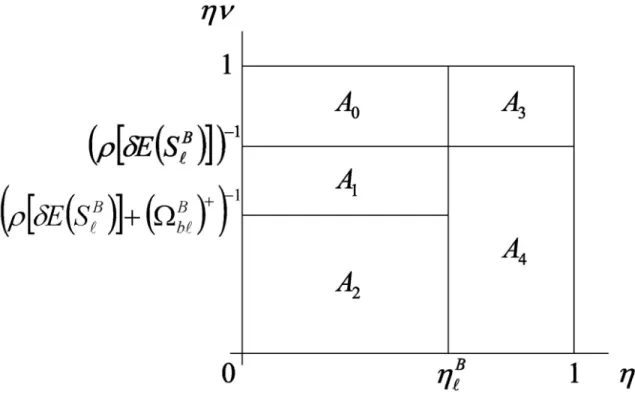
In Figure 1, each agent in the location corresponds to a point in the unit square.29

The agent’s credit score , which equals bank a’s estimate of her type , appears on the horizontal axis. Bankb’s estimate of appears on the vertical axis.30 _While

banka sees only an agent’s horizontal coordinate, bank b sees both.

In the absence of securitization, agents in areas A0 andA3 borrow from bankbat

the interest rate , while other agents do not get loans (Claim 4). With securitization, agents in areas A3 and A4 borrow from bank a at the deterring rate r`B < , while

those in areasA0 and A1 get loans from bank b at the interest rate .

5.1

The E¤ects of Securitization

A comparison of Claim 4 and Theorem 9 reveals the following e¤ects of securitization, which are discussed in section 1.

29_{The applicants are not uniformly distributed throughout the square.}

30_{While the …gure permits and each to take any value in the unit interval, some of these}

Figure 1: E¤ects of Securitization under Limit Irrelevance. A given location ` in region B is depicted. The credit rating appears on the horizontal axis while bank

b’s estimate of an applicant’s type is depicted on the vertical axis. The …gure

assumes that E SB

` >1and Ba`> Bb`>0. Without securitization, applicants in

regionsA0 and A3 receive loans from bank b at the interest rate . Those in regions

A1, A2, and A4 do not receive loans. With securitization, applicants in regions A3

and A4 receive loans from banka at the interest raterB` < . Applicants in regions

A0 andA1 receive loans from bankb at the interest rate , while applicants in region

1. Securitization Stimulates Lending. By connecting agents with liquid in-vestors, securitization expands the set of borrowers.31 _{In Figure 1, areas A}

1

and A4 are added.

2. Securitization Favors Remote Lending. Remote banka lends to location

` only if it can securitize its loans.

3. Remote Borrowers have Strong Observables but High Conditional Default Rates. In Figure 1, the applicants who get remote loans are those whose credit scores exceed bank a’s threshold B

` : they have strong

observ-ables. Now consider an otherwise identical neighborhood`0 in which the bank

a’s securitization pro…ts B

a`0 are higher than in location `. This raises bank

a’s threshold: B_{`</sub>0 > B<sub>`} . The only applicants who are a¤ected are those whose

credit scores lie between the two thresholds. In location `, these applicants all get remote loans. In location `0 they get local loans, but only if bank b’s

estimate of their type is at least E SB

` + Bb`

+ 1

> 0. Thus, ceteris paribus, a remote borrower with a given credit score has an expected type that is no higher, and sometimes strictly lower, than the expected type of a local borrower with the same credit score.

4. Securitization Lets Borrowers with Strong Observables Get Cheap Remote Loans. Securitization lowers the interest rate paid by agents with high credit scores (above B

`) to min ; rB` while leaving unchanged the

in-terest rate paid by agents with lower credit scores.

5. Securitization Raises Conditional and Unconditional Default Rates.

Securitization expands lending to a set of borrowers (in Figure 1, those in areas

A1 and A4) whose expected types are uniformly lower than those of agents

31_{All e¤ects described in sections 5.1 through 5.4 are intended in the weak sense: the set of}

who borrow without securitization (those in areasA0andA3). This raises both

conditional (on ) and unconditional default rates.

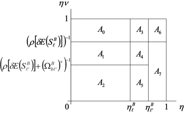
6. Securitized Loans Have Higher Conditional Default Rates then Re-tained Loans. For any given credit score , securitized loans have higher mean default rates than retained loans. More precisely, let us compare two locations ` and `0 _{in regionB. Assume bank b securitizes its loans to location}

`0 but not to location`: B_{b`</sub><0< B<sub>b`}0. In all other respects, the two locations

are identical. The comparison is depicted in Figure 2. For credit scores below

B

` , retained loans consist of areaA0 in location`, while securitized loans consist

of areas A0 and A1 in location `. For each credit score, the securitized loans

have a lower conditional expected type than the retained loans. For credit scores above B

`, all loans are securitized in both locations. Hence, for each

credit score for which there are retained loans in one location and securitized loans in the other, the latter group has a higher conditional default rate.

5.2

Higher Securitization Pro…ts for the Local Bank

Suppose bank b’s securitization pro…ts rise from B

b` to eBb`. Since it is now harder

to deter bankb from cream-skimming, bank a does so less often: it raises its credit score threshold from B

` to e B ` = E(SB `)+(eBb`) + E(SB `)+ Ba`

(equation (14)). Theorem 9 implies the following e¤ects, which are illustrated in Figure 3.

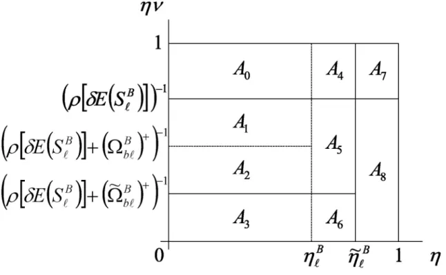
1. Relatively More Local Lending. Bank b lends more, while bank a lends less. In Figure 3, Bankb picks up borrowers in areasA2 andA5. Banka stops

lending to areas A4 throughA6 and is left with only A7 and A8.

2. More Lending to Diamonds in the Rough. The set of borrowers grows to include those with credit scores below a’s threshold B` , whose expected types

Figure 2: Retained Loans Have Lower Expected Default Rates. Two locations `

and `0 _{in region B are depicted. The credit rating appears on the horizontal axis}

while bank b’s estimate of an applicant’s type is depicted on the vertical axis. The …gure assumes that E SB

` = E S`B0 , E S_{`</sub>B > 1, B<sub>a`} = B_a`0 > 0, and

B

b` < 0 < Bb`0. For credit scores below B` , retained loans consist of area A0 in

location `, while securitized loans consist of areas A0 and A1 in location `. For

credit scores above B

` , all loans are securitized in both locations. Hence, for each

credit score , retained loans (if there are any) have a higher expected type than securitized loans.

Figure 3: E¤ect of Increase in Bank b’s Securitization Pro…ts from Bb` to eBb`. The

conditions of Figure 1 are assumed to hold before and after the increase, which raises bank a’s threshold from B` toe

B

` . Bank a, which initially lent to areas A4 through

A8, now only lends to areasA7 andA8 and charges a lower interest rate to this group.

diamonds in the rough: while their credit scores lie below bank a’s threshold, their expected types are the highest among those who previously did not borrow. 3. Welfare Transfer from Good to Great Borrowers (in terms of observ-ables). As bank a no longer competes for agents with credit scores between B `

and _eB` , their interest rate rises from min ; r`B to . However, those with

scores above _eB_` see their interest rate fall since the rate bank a must o¤er to deter bankb is now lower (equation (12)).

5.3

Higher Securitization Pro…ts for the Remote Bank

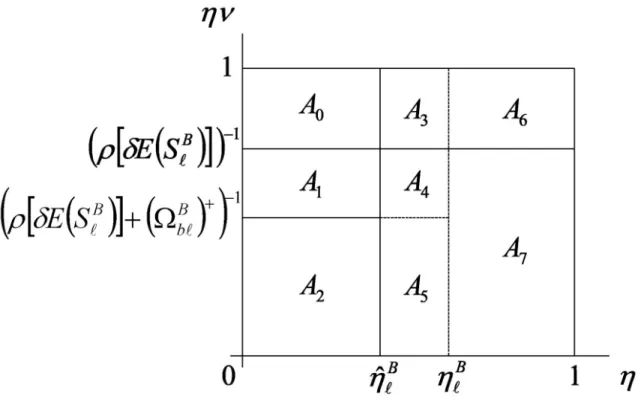
Theorem 9 implies the following the e¤ects of an increase in bank a’s securitization pro…ts from B_{a`</sub> to bB<sub>a`}. These are illustrated in Figure 4, where_bB` denote bank a’s

new, lower credit score threshold.

1. Relatively More Remote Lending. Bank alends more, while bankb lends less. In Figure 4, a picks up borrowers in areas A3 through A5, while b stops

lending to areas A3 and A4 and is left with only A0 and A1.

2. Applicants with High Credit Scores Bene…t from More Loans. The set of borrowers grows to include those with credit scores between banka’s old and new thresholds (areaA5 in the …gure). Among agents who initially did not

get loans, these borrowers have the highest credit scores. These agents bene…t since their interest rate, min ; r_`B , is lower than the project return .

5.4

E¢ ciency E¤ects

We next turn to the e¢ ciency e¤ects of securitization. In order for loans to be allocated e¢ ciently within each location, a resident of location ` in region R must get a loan if and only if her expected project return E SR

` exceeds a

Figure 4: E¤ect of Increase in Bank a’s Securitization Pro…ts from B

a` to bBa`. The

conditions of Figure 1 are assumed to hold before and after the increase, which lowers bank a’s threshold from B

` to b

B

` . Bank b ceases to lend to areas A3 and A4 and

now only lends to areasA0 andA1. Banka adds areasA3 throughA5, andA5 to its

initial borrower pool of A6 and A7. There is no change in the interest rates o¤ered

and regions, this threshold must not depend on the location ` or region R. This is true without securitization, where the threshold cR

` equals

1 _{(Claim 4).}

It is useful to restate the condition for within-location e¢ ciency as follows: an agent gets a loan if and only if her expected type exceeds some location-speci…c threshold_ecR

` .

32 _{This holds without securitization, where only agents in areasA}

0 and

A3 get loans. However, with securitization it fails, since the threshold is zero if an

agent’s credit score exceeds B

` and rB` = >0 otherwise.

This discussion reveals two types of ine¢ ciencies that are caused by securitization. 1. Public Information Bias. Since bank a relies exclusively on public signals to screen agents, there is an ine¢ cient bias towards agents whose public infor-mation is strong. In Figure 1, agents near the top of areaA2, who are turned

down by both banks, are of higher quality than agents near the bottom of area

A4, who get loans from bank a.

2. Securitization Pro…t Bias. E¢ ciency requires that a bank consider only an agent’s creditworthiness. However, in equilibrium a bank also prefers agents who are more pro…table to securitize. For instance, we can reinterpret Figure 3 as comparing two locations in regionB, in which bankb’s securitization pro…ts are B_{b`</sub> and the higher value eB<sub>b`}, respectively. Agents in the top of A2 in the

former location are turned down, while agents in the bottom of the same area in the latter region receive funding. In Figure 4, agents at the top of area A5

are turned down when bank a’s securitization pro…ts are B

a` while agents at

the bottom of the same area receive loans when these pro…ts take the higher value bB

a`. In both cases, e¢ ciency requires the opposite.

32_{In particular,ec}R

` equalscR` E S`R 1