A Join-less Approach for Mining Spatial
Co-location Patterns
Jin Soung Yoo, Student Member, IEEE, and Shashi Shekhar, Fellow, IEEE
Abstract— Spatial co-locations represent the subsets of features which are frequently located together in geographic space. Co-location pattern discovery presents challenges since spatial objects are embedded in a continuous space, whereas classical data is often discrete. A large fraction of the computation time is devoted to identifying the instances of co-location patterns. We propose a novel join-less approach for efficient co-location pattern mining. The join-less co-location mining algorithm uses an instance-lookup scheme instead of an expensive spatial or apriori join operation for identifying co-location instances. We prove the join-less algorithm is correct and complete in finding co-location rules. We also describe a partial join approach for a spatial dataset often clustered in neighborhood areas. We provide the algebraic cost models to characterize the performance dominance zones of the join-less method and the partial join method with a current join-based co-location mining method, and compare their computational complexities. In the experimental evaluation using synthetic and real world datasets, our methods performed more efficiently than the join-based method, and show more scalability in dense data.
Index Terms— Spatial data mining, Association rule, Co-location pattern, Spatial neighbor relationship
I. INTRODUCTION
The explosive growth of spatial data and widespread use of spatial databases emphasize the need for the automated dis-covery of spatial knowledge. Spatial data mining[1], [2] is the process of discovering interesting and previously unknown, but potentially useful patterns from spatial databases. Extracting interesting patterns from spatial datasets is more difficult than extracting the corresponding patterns from traditional numeric and categorical data due to the complexity of spatial data types, spatial relationships and spatial autocorrelation [3].
A spatial co-location represents a subset of spatial features whose instances are frequently located together in spatial neighborhoods. For example, epidemiologists have found that West Nile disease and stagnant water sources are frequently co-located. The co-location rule, i.e., stagnant water source
! West Nile disease, predicts the presence of West Nile
dis-ease in areas with stagnant water sources. Spatial co-location patterns may yield important insights for many applications. For example, a mobile service provider may be interested in service patterns frequently requested by geographically
Manuscript received August 30, 2005; revised May 15, 2006.
Jin Soung YOO(Corresponding Author) is with the Computer Science Department, University of Minnesota, 4-192, EE/CS Bldg., 200 Union Street SE, Minneapolis, MN, 55455, USA (telephone:612-626-7703, e-mail: [email protected])
Shashi SHEKHAR is with the Computer Science Department, University of Minnesota, 4-192, EE/CS Bldg., 200 Union Street SE, Minneapolis, MN, 55455, USA (telephone:612-624-8307, e-mail: [email protected])
neighboring users. The frequent neighboring request sets may be used for providing attractive location-sensitive advertise-ments, recommendations, etc. In another example, ecologists are interested in animal behaviors that frequently co-occur with their nearby environmental or social factors, e.g., food abundance, alpha attack [4]. Other application domains include Earth science, biology, public health, transportation, etc.
Co-location rule discovery is a process to identify co-location patterns from a spatial dataset. Co-co-location rule min-ing presents challenges due to the followmin-ing reasons: First, it is difficult to find co-location instances since spatial objects are embedded in a continuous space and share neighbor rela-tionships. A large fraction of the computation time is devoted to identifying the instances of co-location patterns. Second, it is non-trivial to reuse association rule mining algorithms [5], [6] for co-location pattern mining since, unlike market-basket data, spatial datasets often have no predefined transactions. Thus, a current co-location mining algorithm [7] uses a join-based approach to find co-location instances. Its computational performance suffers, however, due to the large number of joins required as the number of co-location patterns and their instances increases. In this paper, we propose a novel join-less approach for co-location pattern mining which 1) materializes spatial neighbor relationships without any loss of co-location instances, and 2) reduces the computational cost of identifying co-location instances using an instance-lookup scheme.
A. Related Work
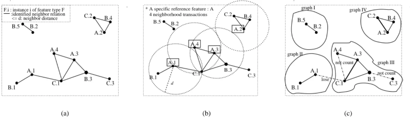
The problem of mining association rules based on spatial relationships (e.g., proximity, adjacency) was first discussed in [6]. The work discovers the subsets of spatial features frequently associated with a specific feature, e.g., cancer. Fig. 1 (a) shows an example dataset with three spatial features, A, B and C. Each object is represented by its feature type and unique instance id, e.g., A.1. Identified neighbor objects are connected by solid lines. Fig. 1 (b) shows the neighbor objects near the objects of a specific reference feature type,A. A set
of neighboring objects of each reference object is converted to a transaction. All rules generated from the transactions are related to the specific feature. However, directly applying this approach to the location mining may not capture our co-location meaning with no specific reference feature.
Previous works on co-location pattern mining have pre-sented different approaches for identifying co-location in-stances and choosing the interest measures of co-location patterns. [8] discovers frequent neighboring class (e.g., co-located features) sets using a support count measure. This
C.2 C.1 B.1 B.3 A.1 A.2 B.4 A.3 B.2 C.3 A.4 B.5 . . <= d: neighbor distance
F.i : instance i of feature type F :identified neighbor relation
(a) C.2 C.1 B.2 B.3 A.1 B.1 A.2 B.4 A.4 C.3 A.3 B.5 d 4 neighborhood transactions * A specific reference feature : A
(b) B.5 B.3 A.1 B.4 A.3 B.2 A.4 C.3 B.1 C.1 C.2 A.2 . . not count graph I graph II graph III graph IV lose not count (c) Fig. 1. (a) An example spatial dataset (b) A reference feature based spatial association rule mining (c) Subgraph mining
approach uses a space partitioning and non overlap grouping scheme for identifying neighboring objects. However, the explicit space partitioning approach may miss co-location in-stances across partitions likefA.4, C.1gin Fig. 2 (a). [7]
pro-posed statistically meaningful interest measures for co-location patterns and a join-based co-location mining algorithm. The instance join operation for generating co-location instances is similar to apriorigen [5]. First, after finding all neighbor
object pairs (size 2 co-location instances), the approach finds size k(>2) co-location instances by joining the instances of
its sizek 1subset co-locations where the firstk 2 objects
are common, and checking the neighbor relationship between
k 1th objects. Fig. 2 (b) shows generating the instances
of co-location fA, B, Cg. This approach finds correct and
complete co-location instance sets. However, the apriori-join operation is computationally expensive with the increase of co-location instances. In the spatial database literature, multi-way join techniques using R-trees for multiple spatial features [9], [10] can be used as alternatives to the apriori-join. However, we assume our spatial dataset has no spatial index, and thus it is difficult to apply these techniques to our co-location mining directly. In our previous work [11], we proposed a partial join algorithm to reduce the number of expensive join operations in finding co-location instances. This approach transactionizes objects using clique neighbor relationships, e.g., posing simple grids in Fig. 2(c), and uses the apriori-join only for the residual instances not modeled by the explicit transactionization. This method reduces the number of join operations significantly. However, its performance depends on the number of cut instances by explicit partitioning.
Co-location pattern mining may appear to be similar with subgraph mining [12], [13], which finds frequent subgraphs in a large graph database. The prevalent interest measure used is support, the ratio of graphs which include a subgraph pattern. For example, in Fig. 1(c), the support of subgraph A C is 2
4
. Subgraph mining is a different problem from our co-location mining, which finds all frequent subsets(i.e., clique subgraphs) from a spatial dataset (i.e., conceptually a single graph which represents input spatial objects and their neighbor relationships). A spatial dataset can be represented to a set of disjoint graphs, and a subgraph mining technique might be applied to it. However, some neighbor relationships can be
lost by the distinct partition, e.g.,fA.1, C.1gin Fig. 1(c), and
the support measure may count one instance in a graph, e.g.,
fA.3, C.1g, but not other instances, e.g., fA.4, C.1g. B. Our Contributions
We took the first step of introducing a join-less algorithm for co-location pattern discovery in [14]. We continue that work here and make the following contributions.
First, we propose to materialize the neighbor relationships
of spatial data for efficient co-location pattern mining. We present two novel neighborhood partition models, star neighborhood partitioning and clique neighborhood partitioning, and compare the models. We also discuss our design decision for co-location instance filtering and prevalent co-location filtering.
Second, we develop a join-less co-location mining
al-gorithm based on the star neighborhood partition model. The algorithm is efficient since it uses an instance-lookup scheme instead of an expensive spatial or instance join operation for filtering co-location instances. It also has a coarse pruning step which can filter candidate co-locations without finding exact co-location instances. We analytically prove our join-less algorithm is correct and complete, i.e., there are no false droppings nor false admissions in finding co-location rules.
Third, we apply the clique partition model to spatial data
especially clustered in neighborhood areas and describe the partial join co-location mining algorithm with a new coarse filtering scheme.
Fourth, we provide algebraic cost models to
ana-lyze the performance dominance zones of the join-less method, the partial join method and a current join-based method [7]. We compare the computational complexity of the different methods.
Finally, we experimentally evaluate our algorithms using
synthetic datasets and real world datasets. The join-less method outperforms the join-based method in overall parameter settings and shows scalability to dense data.
C. Scope and Outline
This paper addresses the co-location pattern mining of spatial point data. We focus on the analytical and experimental
C.2 B.1 B.2 B.3 B.4 A.2 A.4 C.3 A.1 C.1 A.3 B.5 lose . . Vornoi partition (a) C.3 C.1 C.2 A.4 A.3 A.1 A.2 A B C check B.4 C.2 B.3 C.1 A C B.2 join relationships neighbor A.3 B.3 A.1 B.1 A B A.2 B.4 size 3 size 2 size 1 . B.5 B.4 B.3 B.1 B C A B C A.2 B.4 C.2 A.3 B.3 C.1 A.3 C.1 A.4 C.1 A.1 C.1 B.3 C.3 A.2 C.2 (b) C.2 C.1 B.1 B.5 B.2 A.3 B.3 A.1 A.2 B.4 A.4 C.3 .
Trace cut instances . a clique transaction /sqer(2) d /sqer(2)d (c)
Fig. 2. Different approaches for finding co-location instances (a) Space partition (b) Instance join (c) Clique partition and residual instances
comparisons with a current join-based algorithm [7] to ex-amine the effects of our algorithmic design decisions. The discussion of optimized partitioning methods for the clique partition model and the discussion of the significance of co-location interest measures are beyond the scope of this paper. The remainder of the paper is organized as follows. Section II gives an overview of the basic concepts of co-location pattern mining and the problem definition. In Section III, we describe our algorithmic design decision for co-location pattern mining. In Section IV, we present our join-less co-location mining algorithm, and the completeness and correct-ness of the algorithm. In Section V, we describe the partial join method briefly. The analytical analysis of our algorithms and a current join based co-location algorithm is given in Section VI. Section VII presents the experimental evaluation. The conclusion and future work are discussed in Section VIII.
II. CO-LOCATIONPATTERN MINING
In this section, we describe the basic concepts of co-location pattern mining and the problem definition.
A. Basic Concepts
Given a set of spatial features F, a set of their instance
objectsS, and a neighbor relationshipRoverS, a co-location Cis a subset of spatial features,CF, whose instances form
a clique using a neighbor relationship R. When the neighbor
relationshipRis a Euclidean distance metric with its threshold
value, d, two spatial objects are neighbors if they satisfy the
neighbor relationship, i.e.,R(A.1, B.1),(distane(A.1, B.1) d). A co-location instance I is a set of objects, I S,
which includes the objects of all features in the co-location and forms a clique relationship. In Fig. 1 (a),fA.2, B.4, C.2g
is an instance of co-locationfA, B, Cgsince the feature type
of A.2 is A, the feature type of B.4 is B and the feature type of C.2 is C, and R(A.2, B.4),R(A.2, C.2) and R(B.4, C.2).
In this paper, we use the terms ‘instance’ or ‘clique instance’ interchangeably to refer to a co-location instance.
A co-location rule is of the form: C 1 !C 2 (p;p), where C 1 F, C 2 F and C 1 \C 2
= ;. The interest of a
co-location rule can be measured by its prevalence(p) and
condi-tional probability(p). We use the co-location interest measures
defined by [7]. First, the participation ratio Pr(C;f i ) of feature f i in a co-location C = ff 1 ;:::;f k g, 1 i k,
is the fraction of objects of featuref
i in the neighborhood of instances of co-locationC ff i g. It is defined asPr(C;f i )= Numberofdistintobjetsoff
i
ininstanesofC Numberofobjetsoff
i
: The
participa-tion index Pi(C)of a co-location C =ff 1
;:::;f k
g is
de-fined asPi(C)=min f i 2C fPr(C;f i )g. A high participation
index of a co-location indicates that the spatial features of the co-location likely show up together. For example, in the dataset of Fig. 1 (a), feature A has four instances, feature B has five instances, and feature C has three instances. Consider the prevalence values of co-location =fA, B, Cg. The instances
of co-locationarefA.2, B.4, C.2gandfA.3, B.3, C.1g. The
participation ratio of feature A in the co-location,Pr(, A)
is 2 4
since only A.2 and A.3 among four feature A objects are involved in the co-location instances. Pr(, B) is
2 5 and Pr(, C) is 2 3
. Thus the participation index of co-location
, Pi(), is minfPr(, A), Pr(, B), Pr(, C)g = 2 5 . The conditional probabilityP(C 1 jC 2 )of a co-location ruleC 1 ! C
2 is the fraction of instances of C 2 in the neighborhood of instances of C 1. Formally, it is estimated as P(C 1 jC 2 )= NumberofdistintinstanesofC1ininstanesofC1[C2
NumberofinstanesofC 1
. In the example of Fig. 1 (a), the conditional probability of co-location ruleA!ABC,P(AjABC)is
2 4
.
Lemma 1: The participation ratio and the participation
in-dex are monotonically non increasing with increases in the size of the co-location.
For example, the participation index of a size 3 co-location is not greater than the participation index value of any size 2 co-location, e.g., Pi(fA;B;Cg)=
2 5 Pi(fA;Bg)= 3 5 in Fig. 1 (a). Please refer to [7] for the proof of Lemma 1.
B. Problem Definition
We focus on finding a correct and complete set of co-location rules while reducing the computation cost. The formal problem definition is as follows.
Given:
1) A set of spatial feature typesF =ff 1
;:::;f n
g
2) A set of spatial objects S =S 1 [:::[S n where S i (1 in)is a set of instances of feature typef
i. Each object o 2S
i has a vector information of
<feature type f
i, instance
idj and locationx;y >where1j jS i
Spatial dataset Neighbor relationship Prevalence threshold
Conditional probability threshold
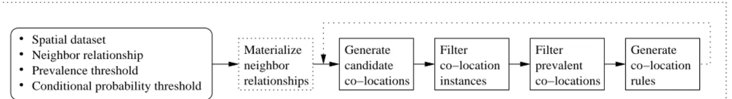
Generate candidate co−locations Generate co−location rules Materialize neighbor relationships Filter co−locations prevalent Filter co−location instances
Fig. 3. Basic procedure of co-location pattern mining
3) A spatial neighbor relationship R
4) A minimum prevalence threshold (min prev) and a
mini-mum conditional probability threshold (minond prob) Find:
A set of co-location rules with participation indexmin prev
and conditional probability min ond prob. Objective:
Find a correct and complete set of co-location rules while reducing the computation cost.
Constraints:
R is a distance metric based neighbor relationship and has a
symmetric property.
III. DESIGNDECISIONS FORCO-LOCATIONPATTERN
MININGALGORITHM
In this section, we present our algorithmic design decisions for the co-location pattern mining.
A. Basic Algorithm
Given a spatial dataset, a neighbor relationship, and interest measure thresholds, the basic co-location pattern mining pro-cedure involves four steps as shown in Fig. 3. First, candidate co-location sets are generated and their co-location instances are gathered from the spatial dataset. Prevalent co-location sets satisfying the given prevalence threshold are filtered. Finally, co-location rules satisfying the conditional probability threshold are generated. Most of the computational time of co-location pattern mining is devoted to finding co-location instances with clique neighbor relationships. Thus we propose to add a step for materializing the spatial neighbor relation-ships to increase the efficiency of co-location mining. In the following subsections, we discuss our design decisions in three areas: neighborhood materialization, co-location instance filtering and prevalent co-location filtering.
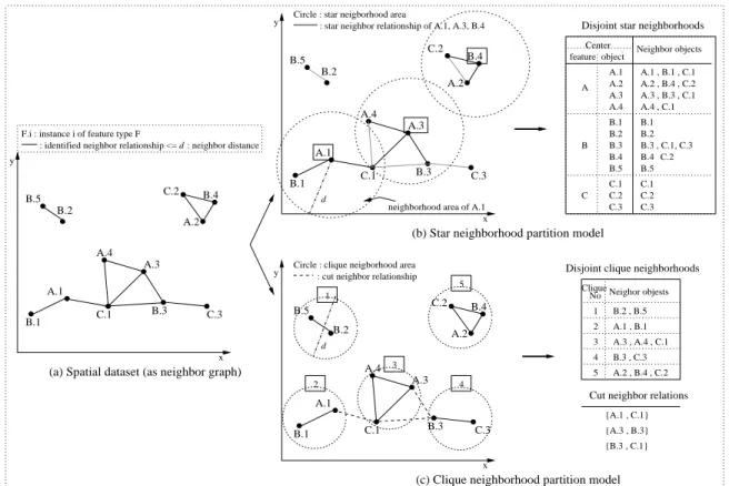
B. Neighborhood Materialization
Given a neighbor relationship, a spatial dataset can be represented as a neighbor graph in which a node is a spatial object and an edge between two nodes represents the neighbor relationship. Fig. 4 (a) depicts a spatial dataset as a neighbor graph. The materialization of neighbor relationships for co-location mining should satisfy two criteria. No neighbor relation should be missed during the materialization process and the computation cost has to be cheap. In addition, it is preferable to minimize duplicate neighbor relations.
We propose two neighborhood materialization models,
star neighborhood partitioning and clique neighborhood partitioning, and then compare them.
B.1. Star neighborhood partition model
The star neighborhood partition model (simply, the star partition model) partitions neighbor relationships using a star neighbor relationship. For example, Fig. 4 (b) shows the possible neighborhood areas of star relationships with objects A.1, A.3 and B.4, which are represented by dotted circles whose radii are a user specific neighbor distance. The black solid lines in each circle represent a star neighbor relationship with the center object. For example, A.1 has a star neighbor relationship with B.1 and C.1. The star partition model can be divided into two types, overlap star partitioning and disjoint
star partitioning. Overlap star partitioning results in duplicate
neighbor relations, e.g., a neighbor relationship between A.1 and B.1 is duplicated in the star relationship of A.1 and in the star relationship of B.1. In contrast, disjoint star partitioning divides the whole neighbor relationships to a set of disjoint star relations. The disjoint star partition model is preferred since it can lead to no duplication nor any loss of neighbor relationships. The star neighborhood of an object identified by the disjoint star partition model is defined as follows.
Definition 1: Given a spatial object o i
2 S whose feature
type is f i
2F, the star neighborhood of o
i is defined as a
set of spatial objects SN = fo j 2Sjo j =o i _(f j >f i ^ R (o j ;o i ))g, wheref j
2F is the feature type of o j and
R is
a neighbor relationship.
The star neighborhood of an object is a set of the center object and objects in its neighborhood whose feature types are greater than the feature type of the center object in a lexical order. In Fig. 4 (b), A.1 has two neighboring objects, B.1 and C.1. The star neighborhood of A.1 is fA.1, B.1,
C.1g including the center object A.1. In the case of A.3,
three neighboring objects, A.4, B.3 and C.1, are present. However, A.4 is not included in the star neighborhood of A.3 since we focus on co-location patterns among different feature types. Next, B.4 has two neighbor objects, A.2 and C.2. However, A.2 is not included in the star neighborhood of B.4 since the neighbor relationship between A.2 and B.4 is already reflected in the star neighborhood of A.2. All star neighborhoods of the spatial dataset are listed in Fig. 4 (b).
B.2. Clique neighborhood partition model
The clique neighborhood partition model (simply, the clique partition model) partitions a spatial dataset into sets of objects having clique relationships. For example, in Fig. 4 (c), A.2, B.4 and C.2 have a clique relationship, and become one partition. The clique partition model can also be divided
B.4 B.5 C.1 B.1 A.3 A.4 A.1 B.3 B.2 A.2 B.4 B.5 C.1 B.1 A.3 A.4 C.3 B.3 C.2 A.1 A.2 C.2 B.2 C.3 B.3 A.4 A.3 C.1 C.3 B.2 A.1 B.1 B.4 A.2 C.2 B.5
Disjoint star neighborhoods
Disjoint clique neighborhoods : cut neighbor relationship
Cut neighbor relations 4 Neighor objests No Clique 1 5
(c) Clique neighborhood partition model (a) Spatial dataset (as neighbor graph)
(b) Star neighborhood partition model
{B.3 , C.1} {A.3 , B.3} {A.1 , C.1} 4 x y d y x x y : star neighbor relationship of A.1, A.3, B.4
d : neighbor distance
F.i : instance i of feature type F
d
neighborhood area of A.1
Neighbor objects
: identified neighbor relationship <=
Circle : star neigborhood area
Circle : clique neigborhood area
object 3 2 feature A.4 A.3 A.2 A.1 A Center A.4 , C.1 A.3 , B.3 , C.1 A.2 , B.4 , C.2 A.1 , B.1 , C.1 3 2 5 B.1 B.2 B.3 B.4 B.5 B B.1 B.2 B.3 , C.1, C.3 B.5 C.2 B.4 C.1 C.2 C.3 C C.1 C.2 C.3 1 B.2 , B.5 A.1 , B.1 A.3 , A.4 , C.1 B.3 , C.3 A.2 , B.4 , C.2
Fig. 4. Neighborhood materialization
into two types, overlap clique partitioning and disjoint clique
partitioning. The overlap clique partitioning generates a set of
maximal cliques. In contrast, the disjoint clique partitioning divides a spatial dataset into a set of disjoint cliques in which each clique is not always maximal. The disjoint clique partition model is preferred since overlap clique partitioning requires finding all maximal cliques, which is computationally expensive(NP-Complete). The following is the definition of a clique neighborhood by the disjoint clique partition model.
Definition 2: A clique neighborhood is a set of spatial
objects CN S that forms a clique under a neighbor
relationshipR. A spatial datasetSis a union of disjoint clique
neighborhoods, fCN 1 ;:::;CN m g whereCN i \ CN j =;, i6=j andCN 1 [:::[CN m =S.
Each spatial object belongs to one clique neighborhood exactly. Fig. 4 (c) illustrates the clique partition model. A dashed circle represents a neighborhood area whose radius is d/2. The objects within the circle are neighbors of each
other. For example, A.1 and B.1 form a clique neighborhood. However, note that this disjoint clique partitioning can lose neighbor relationships across the partitions, e.g.,R(A.1, C.1).
Fig. 4 (c) presents cut neighbor relationships as dotted lines.
fA.1, C.1g, fA.3, B.3g and fB.3, C.1g are the cut neighbor
relations. Our clique partition model also keeps the cut neighbor relations for completeness. Fig. 4 (c) shows a set of the disjoint clique neighborhoods and cut neighbor relations.
B.3. Model Comparison
We compare the star partition model and the clique partition model in terms of their characteristics, the materialized data
size, and advantages and disadvantages in co-location pattern mining. First, if we consider the two models from the per-spective of a graph, the star partition model partitions edges disjointly using a star neighbor relationship. In contrast, the clique partition model partitions nodes disjointly using clique neighbor relationships. The star partition model has n star
neighborhoods, where n is the total number of objects in a
spatial dataset. The number of clique neighborhoods depends on the data distribution. In a declustered spatial dataset where each object is one clique neighborhood, the number of clique neighborhoods isn. In general, the number of clique
neighbor-hoods is much smaller than the number of star neighborneighbor-hoods. Next, we compare the advantages and disadvantages of the models in co-location pattern mining. Star neighborhoods are easily generated from a neighbor graph. However, a star neighborhood does not model a clique relationship directly and can contain ‘false positives’ of co-location instances. In contrast, the cost to generate clique neighborhoods depends on the partitioning method, e.g., from a simple grid partition to a fine partition considering data distribution. The ideal case is to maximize the number of objects in a partition and to minimize the number of cut relationships. The benefit of the clique partition model is that it models clique relationships directly. However, this model requires a procedure to trace ‘false dismissals’ split by the disjoint object partition, i.e., co-location instances related to cut relationships.
C. Co-location Instance Filtering
The algorithmic design for filtering co-location instances from a spatial dataset depends on the neighborhood
mate-rialization model. We present two schemes for co-location instance filtering, instance-lookup and instance-join. We define the following terms to distinguish the instances of co-locations from different neighborhood materialization models.
Definition 3: LetI=fo 1
;::: ;o k
gS be a set of spatial
objects whose feature typesff 1
;:::;f k
g are different. If all
objects in I are neighbors to the first object o 1,
I is called a
star instance of co-location C=ff 1
;:::;f k
g.
For example, in Fig. 4 (b), a subset of A.1 star neighbor-hood, fA.1, B.1g is a star instance of co-location fA, Bg.
Next, we define terms related to the clique neighborhoods.
Definition 4: Let I = fo 1
;:::;o k
g S be an (clique)
instance of co-location C. If all objects in I belong to a
same clique neighborhood,Iis called an intra neighborhood
instance (simply, an intra instance) of co-location C
For example, in Fig. 4 (c), fA.1, B.1g is an intra instance
of co-location fA, Bg.
Definition 5: A neighbor relationship between two objects, o 1 ;o 2 2S;o 1 6=o
2 is called a cut neighbor relationship if o
1 and o
2 are neighbors of each other but belong to different
clique neighborhoods. Definition 6: Let I = fo 1 ;:::;o k g S be an (clique)
instance of a co-locationC. If all objects inIhave at least one
cut neighbor relationship,I is called an inter neighborhood
instance (simply, an inter instance) of co-location C.
For example, in Fig. 4 (c), fA.1, C.1g is an inter instance
of co-location fA, Cg because A.1 has a cut neighbor
relationship with C.1, and C.1 also has cut neighbor relationships with A.1 and B.3. The objects in a inter instance are located across one more clique neighborhoods.
C.1. Instance-lookup
We propose an instance-lookup scheme to filter co-location instances from star instances. A star instance fo
1 ;:::;o k g of co-location ff 1 ;:::;f k
g can be gathered from star
neighborhoods whose center object type isf
1by Definition 3.
Note that the star instance is not a co-location instance since it is not guaranteed that it has a clique relationship. However, if all objects in it except the first object(the center object of the star relationship) form a clique, the star instance is a co-location instance. The cliqueness of the subset can be checked by searching other star instances, e.g., the second object o 2’s star instance, fo 2 ;:::;o k
g, the third object o 3’s
star instance, fo 3
;:::;o k
g, etc., or by looking up the clique
instances of co-location ff 2 ;:::;f k g exceptf 1. C.2. Instance-join
Intra neighborhood instances (i.e., instances within neigh-borhoods) can be gathered by scanning the clique neighbor-hood set. An intra instance is a co-location instance since a subset of a clique neighborhood is also a clique. In contrast, inter neighborhood instances (i.e., instances over different neighborhoods) are not found from the materialized set di-rectly. We adopt an instance join method [7] for tracking the inter instances. The inter instances of a size k co-location
can be generated by joining the inter instances of its size
k 1 co-locations. For example, in Fig. 4 (c), an inter
instance fA.3, B.3, C.1g can be generated by joining size 2
inter instances, fA.3, B.3gandfA.3, C.1g, and checking the
neighbor relationship between B.3 and C.1.
D. Co-location Filtering
We use three filtering steps to find prevalent co-locations:
feature-level filtering, coarse filtering and refinement filtering.
Feature-level filtering is possible due to the anti-monotonic property of participation index by Lemma 1. A candidate co-location can be pruned without examining its instances if any subset of it is not prevalent. Coarse filtering is done after finding all star instances or after finding all intra instances of co-locations, which depends on the materialization model. This step can reduce the expensive filtering operation for co-location instances. If the prevalence value of star instances of a candidate co-location does not satisfy a given threshold, the candidate is pruned without the cliqueness check of its star instances. In the clique partition model, the intra instances of a candidate co-location do not give enough information for the coarse pruning. Thus we use cardinal objects from the inter instances of its subsets as well as its intra instances. If the prevalence value from them does not satisfy the threshold, the co-location is pruned without finding its inter instances. In the last step, the refinement filtering decides prevalent co-location sets after filtering all co-location instances.
E. Design Decision
The choice of the neighborhood materialization models can depend on the distribution of input spatial data. For general spatial datasets, we choose the star neighborhood partition model and use the instance lookup scheme for filtering co-location instances. We present the join-less co-co-location mining algorithm in the next section. In contrast, the clique partition model is appropriate for spatial data mostly clustered in neighborhood areas having fewer neighbor relationships with their nearby neighborhoods. This is because clustered data can be modeled to clique neighborhoods and fewer neighbor inter-actions with nearby neighborhoods can reduce the number of cut relationships. The partial join approach is briefly discussed in Section V.
IV. JOIN-LESSAPPROACH
In this section, we present a join-less co-location mining
algorithm based on the star neighborhood partition model.
We show the algorithm is correct and complete in mining co-location patterns.
A. Join-less Co-location Mining Algorithm
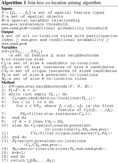
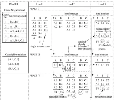
The join-less co-location mining algorithm has three phases. The first phase converts an input spatial dataset into a set of disjoint star neighborhoods. The second phase gathers the star instances of candidate co-locations from the materialized set, and coarsely filters the candidates using the prevalence values of their star instances. The third phase filters their co-location instances from the star instances, and finds prevalent co-locations and generates co-location rules. The second and third phases are repeated with the increase of co-location size. Fig. 5 illustrates a trace example of the join-less algorithm. Algorithm 1 shows the pseudo code. The detailed explanation is given as follows.
A.4 , C.1 B C B.3 , C.1 B.3 , C.3 B.4 , C.2 A.1 , B.1 A.2 , B.4 A.3 , B.3 A B A C A.1 , C.1 A.2 , C.2 A.3 , C.1 A.4 , C.1 4/4 2/3 B C B.3 , C.1 B.3 , C.3 A.3 , C.1 PHASE I 4 PHASE II B B.1 B.2 B.3 B.4 B.5 C C.1 C.2 C.3
single instance count Feature B star neighborhoods
Feature C star neighborhoods 5 A C A.1 , C.1 A.2 , C.2 B.4 , C.2 , B.4 , C.2 A.3 , B.3 , C.1 A B C 2/5 2/3 true participation index PHASE III Level 3
if < threshold, it’s pruned on star instances Check if it is a clique 3 A.2 2/5 3/3 A.1 , B.1 , C.1 A.2 , B.4 , C.2 A.3 , B.3 , C.1 A B C star instances 3/4 3/5 2/3 participation index instances clique 2/4 A.1 , B.1 , C.1 Feature A star neighborhoods
A B A.3 , B.3 A.4 , C.1 A.3 , B.3 , C.1 A.2 , B.4 , C.2 A.1 , B.1 , C.1 B.1 B.2 B.3 , C.1, C.3 B.5 C.2 B.4 C.1 C.2 C.3 3/5 3/4 A.1 , B.1 A.2 , B.4 Level 2 A A.1 A.2 A.3 A.4 Level 1
Fig. 5. An illustration of the join-less co-location mining algorithm
1) Convert a spatial dataset to a set of disjoint star neighborhoods (Step 1): Given an input spatial dataset and
a neighbor relationship, first find all neighboring object pairs using a geometric method such as plane sweep [15]. The star neighborhoods can be generated from the neighbor pairs by grouping the neighbor objects per each object. Fig. 5 shows the same star neighborhood set in Fig. 4 (b).
2) Generate candidate co-locations(Step 4): First, we
ini-tialize all features to size 1 prevalent co-locations by the defi-nition of participation index. The number of instances per each feature can be known during the neighborhood materialization procedure. Sizek(k>1) candidate co-locations are generated
from prevalent size k 1 co-locations(step 4). Here, we have
the feature level filtering of the co-locations. If any subset of a candidate location is not prevalent, the candidate co-location is pruned.
3) Filter the star instances of candidate co-locations from the star neighborhood set(Step 5): The star instances of a
candidate co-location are gathered from the star neighborhoods whose center object’s feature typ is the same as the first feature of the co-location. For example, the instances of co-location
fB, Cg are gathered from the feature B star neighborhoods,
and the instances of co-location fA, B, Cgare gathered from
the feature A star neighborhoods. Notice that the number of candidate co-locations examined in each star neighborhood is much smaller than the number of actual candidates.
4) Select coarsely prevalent co-locations using their star instances(Step 10): The size 2 star instances are clique
in-stances since our neighbor relationship is symmetric. Thus, we go to step 13 to find prevalent co-locations. For size 3 or more, we need to check if the star instances are clique instances. Before this procedure, we have a coarse filtering of the co-locations. We filter a candidate co-location using the participation index of its star instances. For example, in Fig. 5, the participation index of candidate co-location fA, B,
Algorithm 1 Join-less co-location mining algorithm
Inputs
F=ff 1
;:::;f n
g:a set of spatial feature types S:a set of spatial objects
R:a spatial neighbor relationship minprev:prevalence threshold,
minondprob:conditional probability threshold
Output
A set of all co-location rules with participation index minprev and conditional probability minondprob
Variables SN=fSN f1 ;:::;SN fn g :a set of feature f i star neighborhoods k:co-location size
Ck:a set of size k candidate co-locations SIk:a set of star instances of size k candidates CIk:a set of clique instances of sizek candidates Pk:a set of size k prevalent co-locations
Rk:a set of size k co-location rules
Method
1) SN=gen star neighborhoods(F, S, R); 2) P1=F; k = 2;
3) while (not empty P
k 1) do
4) Ck=gen candidate co-locations(P k 1); 5) for i in 1 to n do 6) for t 2SN f i where f i =f1, f 1 is the first feature of C k (f 1 ;:::;f k ). 7) SIk=filter star instances(C
k ;t); 8) end do 9) if k = 2 then CI k =SI k
10) else do Ck=select coarse prevalent co-locations(C
k ;SI
k
;minprev) 11) CIk=filter clique instances(C
k ;SIk); 12) end do
13) Pk=select prevalent co-locations (C
k ;CI
k
;minprev); 14) Rk=gen co-location rules(P
k
;minondprob); 15) k=k+1; 16) end do 17) return S (R 2 ;:::;R k );
Cgfrom its star instances is 3 5
. If it is less than a user specified minimum prevalent threshold, the candidate is pruned without examining exact co-location instances.
5) Filter co-location instances(Step 11): From the star
instances of a candidate co-location, we filter its co-location instances using the instance look-up scheme. For example, in Fig. 5, to check the cliqueness of a star instance fA.1, B.1,
C.1g of co-locationfA, B, Cg, we examine if a sub instance fB.1, C.1g except A.1 is in the set of clique instances of
co-location fB, Cg. This instance look up operation can be
performed efficiently by an instance key which is composed of the ids of objects in the instance. As shown in Fig. 5,fA.1,
B.1, C.1g is not a co-location instance, but fA.2, B.4, C.2g
andfA.3, B.3, C.1gare co-location instances.
6) Select prevalent co-location sets(Step 13): The
refine-ment filtering of co-locations is done by the true participation index values calculated from their co-location instances. Preva-lent co-locations satisfying a given threshold are selected.
7) Generate co-location rules(Step 14): Finally we
gen-erate all co-location rules satisfying a given minimum condi-tional probability from a set of prevalent co-locations. Steps 3-16 are repeated as the co-location size increases.
B. Completeness and Correctness
Completeness means the join-less algorithm finds all co-location rules whose participation index and conditional
prob-ability satisfy a user specified minimum prevalence threshold and conditional probability threshold. Correctness means that all co-location rules generated by the join-less algorithm have participation index and conditional probability values above the minimum thresholds. First we provide related lemmas.
Lemma 2: The star partition model does not miss any
neighbor relationship of an input spatial dataset.
Proof: The disjoint star partition model includes all
neighbor relations of each object and excludes only dupli-cate neighbor relations which are already included in a star neighborhood by Definition 1. Lemma 3: Let C = ff 1 ;:::;f k g be a size k co-location
andSI be the star instances ofC. The participation index of C from SI is not less than the true participation index ofC.
Proof: The participation ratio of f 1 from
SI is the
maximum possible probability that the objects of feature f 1
have clique relationships with the objects of the other features
f 2
;::: ;f k in
C since only objects of feature f
1 in the star
instances can be included in the clique co-location instances of C. The participation ratio of f
j(
2 j k) from SI
is also the maximum possible probability that the objects of feature f
j have clique relationships with the objects of
features f
1 since our neighbor relationship is symmetric.
Thus the participation index of C calculated from the star
instances is not less than the true participation index ofC, i.e., min f i 2C fpossiblemaxPr(C;f i )g min f i 2C fPr(C;f i )g. Lemma 4: Let an instance I = fo
1 ;:::;o k g be a star instance of co-locationC=ff 1 ;:::;f k
g. If the sub instance fo 2 ;:::;o k gexcepto 1 is a clique, Iis a co-location instance of C.
Proof: In a star instanceI=fo 1
;:::;o k
g, the first object o
1has neighbor relationships to the other objects, o 2 ;:::;o k, by Definition 3. If a subset fo 2 ;::: ;o k g is a clique, object o j(
2 j k) has neighbor relationships with all objects
in the subset as well as o 1. Thus
I is a clique co-location
instance.
Theorem 1: The join-less co-location mining algorithm is
complete.
Proof: The completeness of the join-less algorithm can be
shown in two ways. The first is that the method to materialize the neighbor relationships of an input spatial dataset (step 1), the method to gather star instances(step 7), and the method to filter clique instances(step 11) are correct. The star partition model does not miss any neighbor relationship of the input data by Lemma 2. The star instances gathered from the star neighborhoods where the feature type of the center object is the same with the first feature of the co-location have correct star neighbor relationships by Definition 1 and 3. Any potential co-location instance is not missed since the star instances are a super set of the clique instances. The method to filter co-location instances from the star instances does not drop a true instance by Lemma 4. Next, we show that the filtering steps of locations do not miss true co-locations. The feature level filtering by prevalent subsets(step 4) is complete by Lemma 1. The coarse filtering(step 10) does not eliminate any true prevalent co-locations by Lemma 3. The refinement filtering(step 13) prunes only co-locations whose
Clique Neighborhood
Cut neighbor relations Neighoring objests No C C.1 C.2 C.3 3 inter instances A C A.1 C.1 A.3 C.1 A C A.1 C.1 A.4 C.1 A.2 C.2 A.3 C.1 A B A B A.1 B.1 A.2 B.4 Clique Level 1 Level 2 PHASE II intra instances A C A.3 C.1 A.4 C.1 A.2 C.2 A B A.1 B.1 A.2 B.4 B C B.3 C.3 B.4 C.2 PHASE I 2 3 4 5 1 A.3 B.3 estimated inter inter instances A.2 B.4 C.2 A B C A.3 B.3 C.1 A B C A.3 B.3 C.1 2/4 2/5 2/3 participation index Level 3 intra instances A.3 B.3 C.1 2/4 2/5 2/3 if < threshold, pruned.. PHASE III PHASE IV instance objects A.3 B.3 B C B.3 C.1 B C B.3 C.1 B.3 C.3 B.4 C.2 3/4 3/5 2/3 4/4 2/5 3/3 {A.1 , C.1} {A.3 , B.3} {B.3 , C.1} participation ratios join single instance count
A.2 B.4 C.2 A B C objects from size 2 inter instances cardinal B.2 , B.5 A.1 , B.1 A.3 , A.4 , C.1 B.3 , C.3 A.2 , B.4 , C.2 A A.1 A.2 A.3 A.4 4 B B.1 B.2 B.3 B.4 B.5 5
Fig. 6. An illustration of the partial join co-location mining algorithm
true participation index is less than the threshold. Step 14 ensures that no co-location rules satisfying a given conditional probability are missed.
Theorem 2: The join-less co-location mining algorithm is
correct.
Proof: The correctness of the join-less algorithm can
be guaranteed by steps 13 and 14. Step 13 selects only co-locations whose participation indexes satisfy a user specific prevalence threshold. The generated co-location rules by step 14 also satisfy a user specific conditional probability.
V. PARTIALJOINAPPROACH
In this section, we briefly describe a partial join approach for spatial datasets that are mostly clustered in neighborhood areas with fewer neighbor relationships with their nearby neighborhoods. The partial join co-location mining algorithm was proposed in our previous work [11]. Here we added a coarse filtering scheme to further reduce the number of join operations. The partial join approach uses the clique partition model for materializing clustered data to clique neighborhoods directly, and keeps track of co-location instances split by the disjoint object partitioning. Fig. 6 (b) shows a trace example of the partial join co-location mining algorithm.
Given a spatial dataset and a neighbor relationship, first we need to generate a set of disjoint cliques. To do this, we use grid partitioning. The rectangular grids of size d=
p 2 d=
p
2, wheredis a neighbor distance, are posed on a spatial
framework. The objects in each grid are generated to a clique neighborhood. Cut neighbor relations can be detected by examining neighbor pairs whose partition areas are different. Size 2 inter instances(i.e., instances across neighborhoods) are the cut relations and the pairs of objects having at least one cut neighbor relationship in each partition. The intra instances(i.e., instances within neighborhoods) of a sizek(k>2) candidate
co-location are enumerated from the clique neighborhood set. For example, in Fig. 6,fA.2, B.4, C.2gis an intra instance of
co-location fA, B, Cg. Before finding the inter instances of a
candidate location, we conduct a coarse filtering of the co-location using its intra instances and the cardinal objects from the inter instances of its sizek 1co-locations. For example,
in Fig. 6, the cardinal objects which can be involved in the inter instances of co-location fA, B, Cgare A.3 of feature A,
B.3 of feature B and C.1 of feature C. If the participation index calculated from them does satisfy a given threshold value, we further go to find the exact inter instances. We use an instance join method [7] for generating the inter instances. For example, the inter instances of fA, B, Cg are produced
by joining an inter instance offA, Bg,fA.3, B.3gand an inter
instance offA, Cg,fA.3, C.1g, and by examining the neighbor
relationship between B.3 and C.1. The true participation index of a co-location is calculated from its intra instances and inter instances. All co-location rules whose prevalence value and conditional probability satisfy given thresholds are generated.
VI. ANALYTICALCOMPARISON
In this section, we analytically compare our join-less and partial join location algorithms with a pure join-based co-location algorithm [7]. First we examine the computational complexities of the different methods and then compare them.
A. Computational Complexities Let T jl, T pj and T
jb be the total computation cost of the
join-less method, the partial join method, and the join-based method, respectively. The following equations show the total cost functions. T jl = T starneighborhoods (S)+ T jl (2) + P k>2 T jl (k) T pj = T
l iqueneighborhoods&utrel ations (S)+ T pj (2) + P k>2 T pj (k) T jb = T neighborpairs (S)+T jb (2)+ P k>2 T jb (k)
S denotes an input spatial dataset. T jl (2), T pj (2) and T jb
(2) represent the cost for finding size 2 co-location
patterns in each method. The following equations are the costs of finding sizek(k>2) co-location patterns.
T jl (k)= T genandi (P k 1 )+ T
fil terstarinst (C
k )
+ T
fil teroarseol o (C
k )+ T
fil terl iqueinst (C
0 k )
+ T
fil terprevol o (C 0 k )+ T genrul es (P k ) T
fil terstarinst (C
k )+ T
fil terl iqueinst (C 0 k ) T pj (k)=T genandi (P k 1 )+T
fil terintrainst (C
k )
+ T
fil teroarseol o (C
k )+ T
fil terinterinst (C
00 k )
+ T
fil terprevol o (C 00 k ) +T genrul es (P k ) T
fil terintrainst (C
k )+ T
fil terinterinst (C 00 k ) T jb (k)=T genandi (P k 1 )+T
fil terinst (C
k )
+ T
fil terprevol o (C k )+ T genrul es (P k ) T
fil terinst (C
k )
P
k 1 is a size
k 1prevalent co-location set,C
k is a size k candidate co-location set, and each C
0 k and C 00 k is a size
k candidate co-location set filtered by the coarse filtering in
the join-less algorithm and the partial join algorithm. In these equations, T
genrul es is the same cost in all three methods. T
genandi, T
fil teroarseol o and T
fil terprevol o can be
ignored when compared with other computation factors as shown in the experiment results of the next section.
B. Comparison of Computational Complexities
We compare the computational complexities of the different methods in two parts. One is the computation cost of material-izing neighborhoods and generating size 2 co-location patterns and, the other is the computational cost of generating size
k(k>2) co-location patterns.
1) Neighborhood materialization & size 2 co-locations :
The computational costs of materializing neighborhoods and generating size 2 co-location patterns in the different methods are compared by the following equation.
T
l iqueneighborhoods&utrel ations (S)+T pj (2) >T starneighborhoods (S)+T jl (2) >T neighborpairs (S)+T jb (2)
First, each method needs to find all neighboring pairs. The cost is the same in the three methods. The join-based method generates size 2 co-locations by gathering the neighbor pairs per candidate co-location, and calculating their prevalence measures. In both the join-less method and the partial join method, the size 2 co-locations can be found also from the neighbor pairs or by scanning their materialized neighborhood set. If we use the former, the cost is the same in all three methods. However, the join-less method has an additional cost to materialize the star neighborhoods from the neighbor pairs. In the partial join method, we generate the disjoint clique neighborhoods using a simple grid partitioning. The cut relations are also easily found during the neighbor pair search, but an additional cost is required to find all size 2 inter instances with cut relationships. The overall cost is expected to be a litte bigger than the cost to generate the star neighborhood set.
2) Join-less vs. Join-based with sizek(k>2) co-locations:
We compare the join-less algorithm with the join-based al-gorithm in generating size k(k > 2) co-location patterns.
Equation (1) shows the computation ratio.
T jl (k) T jb (k) T
fil terstarinst (C
k )+T
fil terl iqueinst (C
0 k )
T
fil terinst (C k ) jC k jt san +p jl jC k jt l ookup jC k jt join t san +p jl t l ookup t join (1) t
sanis the average cost to collect the star instances of a
can-didate co-location by scanning the materialized neighborhood set.p
jl is the coarse filtering ratio. t
l ookup is the average cost
to check the cliqueness of its star instances.t
joinis the average
cost to generate co-location instances per co-location using the instance join. If the input dataset is dense,t
san t join and the ratio isp jl t look up t join
. We assume that the number of instances involved in the join operation and the number of instances involved in the lookup operation per co-location is similar. Even if the coarse pruning is not effective(p
jl=1), the join-less
algorithm is expected to take less computation time than the join-based algorithm since t
l ookup < t
join. We examine the
efficiency oft
l ookup over t
joinwith different density datasets
the number of instances involved in the join operation or the lookup operation increases and the computation difference betweent
l ookupand t
joinis expected to be bigger. The overall
data density is controlled by spatial frame size, and the coarse filtering ratiop
jlis controlled by an overlap parameter, which
is the ratio of the number of points included in different co-location instances over the total number of points.
3) Partial-join vs. Join-based with size k(k > 2) co-locations : T pj (k) T jb (k) T
fil terintrainst (C
k )+T
fil terinterinst (C
00 k )
T
fil terinst (C k ) jC k jt san (intraI)+p pj jC k jt join (interI) jC k jt join (I) t san (intraI)+p pj t join (interI) t join (I) (2)
In equation (2),intraI is the intra instances from the clique
neighborhoods, interI is the inter instances joined in the
partial join method and I is the instances joined in the
join-based method. In general, t san
(intraI) t join
(I) since
the cost of gathering instances by scanning a neighborhood materialization set is much cheaper than the join operation for generating whole instances. The number of inter instances in the partial join method is a major factor in this ratio. If jinterIj jIj, the partial join method is expected to
have less computation cost. If jinterIj 'jIj and the coarse
pruning is not effective(p pj=1), t join (interI)'t join (I)and t san
(intraI) cost is added to the partial join method. The
join-based method is expected a little better. To control the number of inter instances in the experiment, we use anaross
ratio which is ratio of instances across different neighborhood areas over total instances.
4) Join-less vs. Partial-join with sizek(k>2) co-locations:
T jl (k) T pj (k) T
fil terstarinst (C
k )+T
fil terl iqueinst (C
0 k )
T
fil terintrainst (C
k )+T
fil terinterinst (C 00 k ) p jl jC k jt l ookup (I) p pj jC k jt join (interI) p jl t l ookup (I) p pj t join (interI) (3) In dense data, T
gatherstarinst (C
k
) and
T
gatherintrainst (C
k
) are expected relatively smaller
than other factors. If we assume the coarse filter ratios are the same, the comparison of the two methods is the same with the comparisons of T
l ookup and T
join, and of
jIj and jinterIj. In datasets of dense in neighborhoods with fewer
inter instances, the partial join method is expected to show better performance. In the experiment presented later, we compare the behavior of the two algorithms in data density in neighborhood area and the ratio of cut instances. Each factor is controlled by clumpy degree and across ratio variables.
VII. EXPERIMENTALEVALUATION
We evaluate the join-less and the partial join co-location algorithms with the join-based algorithm [7] using synthetic and real datasets. We conducted the following experiments.
We examined the effects of our algorithm design
deci-sions. Specifically, we compared the computation costs of generating up to size 2 co-location patterns with and without a materialization step. We examined the efficiency of the instance-lookup scheme, and the effect of coarse filtering. In addition, we compared the costs of the computation complexity factors of the three algorithms to support our analytical comparisons in Section VI.
We examined the scalability of the join-less algorithm in
terms of the number of points, the number of features, the distance neighbor threshold, and the prevalence threshold.
We examined the behavior of the partial join algorithm
with different neighborhood densities and cut relation ratios.
Finally, we evaluated the algorithms with two real
datasets, a climate dataset and an Ecology dataset. All algorithms were implemented in C/C++, and are memory based algorithms. All the experiments were performed on a Sun SunBlade 1500 with 1.0 GB memory and 177MHz CPU.
A. Synthetic Data Generation
Synthetic datasets were generated using a spatial data gen-erator similar to [7]. Table I describes the parameters used for the data generation. First, overall spatial frame size is determined with the frame side lengthD. ADDsize frame
was used. The whole frame was divided into regular grids whose side length was a neighborhood distance d. In order
to generate co-location instances located across the grids, we divided each grid into two areas, a non-overlapping area and an overlapping area. An object in the non-overlapping area has neighbor relationships only with other objects in the same area. By contrast, objects in the overlapping area can have neighbor relationships with objects in the nearby grids.
The following is the procedure we used to generate gen-eral synthetic datasets in which co-location instances were randomly distributed. First we generated P initial patterns
whose average size wasS. The feature types of each pattern
were randomly chosen fromF features. AverageI instances
per each pattern were generated. The total number of points was N. For locating a co-location instance, first we chose a
grid cell randomly. All points of the instance were randomly located within the chosen grid cell.
To generate our specialized datasets, first, overall data density was controlled by spatial frame sizeDD. Under a
fixed total number of points, a smaller frame generates more dense data. Second, the data density in neighborhood areas was controlled by a lumpy degree. When a new grid cell
was chosen randomly for locating a co-location instance, a
lumpy number of instances was generated in the same grid
cell. The defaultlumpyvalue was 1. Third, thearossratio
controlled the number of instances across different grid cells. An across instance was generated in the overlapping area of a chosen grid and its nearby grid. Finally, the number of points overlapped in different co-location instances was controlled by theoverlapratio.Noverlappoints were randomly selected.
Eachoverlappoint was involved in four co-location instances.
The parameter values for the synthetic dataset used in each experiment are described in Table I.
Experiment no.
Symbols Meaning 1-1 1-2 1-3 1-4 2-1 2-2 2-3 2-4 3-1 3-2
S Average size ofyco-locations 5
P Number ofyco-locations 20
I Average number ofyco-location instances 150
F Number of features 20 * 20
N Number of points 15K * 15K
D Spatial frame size(DD) * 5000 10000, 1000 5000 10000
d Neighborhood distance threshold 10 * 10
Prevalence threshold 0.3 0.2 0.3 * 0.3
lumpy Number of co-location instances
generated in a same neighborhood area 1 * 15
aross Ratio of instances across different
neighborhood areas over total instances 0 10 *
overlap Ratio of points overlapped in different
co-location instances over total points 0 * 0
y: initial core co-location, * : variable values
TABLE I
EXPERIMENTALPARAMETERS AND THEIR VALUES IN EACH EXPERIMENT
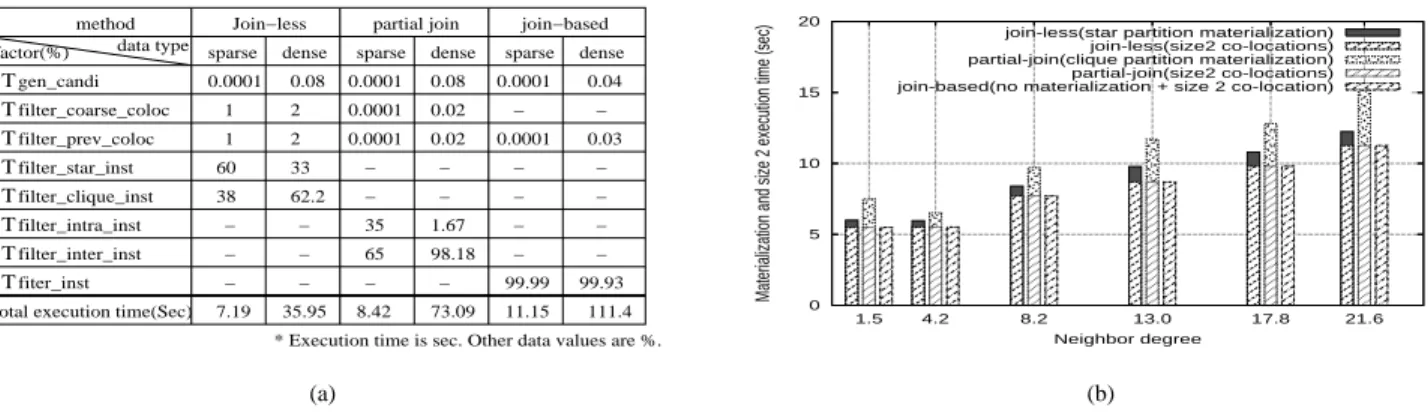
65 0.0001 0.0001 33 2 2 0.08 38 60 1 1 0.0001 method sparse dense sparse dense join−based partial join Join−less sparse dense 35
total execution time(Sec) factor(%) data type
* Execution time is sec. Other data values are %. 99.93 0.03 0.04 62.2 35.95 8.42 73.09 1.67 98.18 0.02 0.02 99.99 0.0001 0.0001 0.0001 111.4 11.15 7.19 0.08 − T T T − − − − − − − − − − − − − − − − − − − − − T Tfiter_inst filter_inter_inst filter_intra_inst filter_clique_inst filter_star_inst filter_prev_coloc gen_candi filter_coarse_coloc T T T (a) 0 5 10 15 20 21.6 17.8 13.0 8.2 4.2 1.5
Materialization and size 2 execution time (sec)
Neighbor degree
join-less(star partition materialization) join-less(size2 co-locations) partial-join(clique partition materialization) partial-join(size2 co-locations) join-based(no materialization + size 2 co-location)
(b)
Fig. 7. (a) Computation of computational complexity factors (b) Computation comparison of neighborhood materialization and size 2 co-location generation
B. Experiment Results
We present a summary of our experiment results.
B.1. Effects of algorithm design decision
1) Comparison of computational complexity factors: We
examined the costs of the computational complexity factors discussed in Section VI. We used two datasets of different density, i.e., a sparse dataset with neighbor degree 5 and a dense dataset with neighbor degree 15. In Fig. 7 (a), data values except total execution time represent percent values. Overall, we can notice thatT
genandi, T
fil teroarseol o and T
fil terprevol o take much less portion than the other costs.
In addition, T
fil terstarinstand T
fil terintrainstof gathering
instances from each materialization set are relatively smaller than T
fil terinterinst and T
fil terinst using instance join
op-erations. The difference is greater in the dense dataset.
2) Comparison of neighborhood materialization methods:
We compared the computation cost of generating up to size 2 co-locations, including the costs of neighborhood materializa-tion. Size 2 co-locations were generated from neighboring ob-ject pairs in all methods. Fig. 7 (b) shows the execution times of three approaches, with star partition materialization, with clique partition materialization, and with no materialization. As can be seen, the join-less approach without materialization shows less execution time. In the materialization methods, the
star partitioning of join-less approach took less computation time than the clique partitioning of partial join approach.
3) Comparison of instance filtering methods: We examined
the efficiency of our instance look-up scheme over the instance join method in the join-based algorithm with different dense datasets. Data density determines the neighbor degree of an object, which in turn affects the number of co-location instances. Neighbor degree is the average number of neighbor points per each point. Different spatial frame sizes were used to control the overall data density of the same number of points. Fig. 8 (a) compares the execution time of finding size 3 or more co-location instances of the different schemes. We turned off the coarse filtering option to see only the effects of instance filtering schemes. In sparse datasets(e.g., neighbor degree<10), the two methods show similar execution time.
However, the execution time increases as the neighbor degree increases, and here the instance-lookup method shows better performance than the instance-join method. Moreover, the difference in execution times of the two methods is much greater with the increase of neighbor degree.
4) Effect of coarse pruning: We examined the effect of the coarse filtering scheme in the join-less algorithm. Fig. 8 (b) shows the percent of candidate co-locations pruned in the coarse filtering step over the total candidate co-locations after the feature-level pruning. We considered only size 3
0 50 100 150 200 5 10 15 20
Size 3 or more execution time (sec)
Neighbor degree join-less(instance-lookup) join-based(instance-join) (a) 0 20 40 60 80 100 0 5 10 15 20 Pruning ratio(%) Overlap ratio(%) (b) Fig. 8. (a) Comparison of instance filtering schemes (b) Effect of coarse pruning in the join-less method
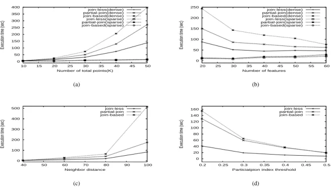
0 50 100 150 200 250 300 350 400 10 15 20 25 30 35 40 45 50
Execution time (sec)
Number of total points(K) join-less(dense) partial-join(dense) join-based(dense) join-less(sparse) partial-join(sparse) join-based(sparse) (a) 0 50 100 150 200 250 20 25 30 35 40 45 50 55 60
Execution time (sec)
Number of features join-less(dense) partial-join(dense) join-based(dense) join-less(sparse) partial-join(sparse) join-based(sparse) (b) 0 100 200 300 400 500 40 50 60 70 80 90 100
Execution time (sec)
Neighbor distance join-less partial-join join-based (c) 0 20 40 60 80 100 120 140 160 0.2 0.25 0.3 0.35 0.4 0.45 0.5
Execution time (sec)
Particiatpion index threshold join-less partial-join join-based
(d)
Fig. 9. Scalability of the join-less algorithm (a) by number of points (b) by number of features (c) by neighbor distance (d) by prevalence threshold
or more candidates since the coarse pruning is effective in filtering them. With the increase of overlap ratio, the chance of pruning the candidate co-locations increased since the participation ratios of features of overlap points decrease.
B.2. Scalability of the join-based algorithm
We examined the scalability of the join-less algorithm with several workloads, i.e., the number of point objects, the number of feature types, distance neighbor threshold, and prevalence threshold. We compared the total computation time of finding all prevalent co-locations including the materializa-tion cost.
1) Effect of the number of point objects: First, we compared
the effect of the number of points in the different algorithms. We used two different spatial frame sizes, 10;00010;000
and1;0001;000. In the first frame, even if the number of
points is increased from 10K to 50K, the three algorithms showed similar execution time since the datasets are still sparse. However, in the second frame, with the increase of number of points, the join-based algorithm’s execution time is
dramatically increased due to the increase of data density. As shown in Fig. 9 (a), the join-less algorithm shows scalability to large dense datasets.
2) Effect of the number of features: In the second
exper-iment, we compared the performance of the algorithms as a function of the number of different features. We also used two different dense datasets of 15K points. Fig. 9 (b) shows the results. In the sparse dataset, the algorithms show similar execution time even if the number of features increases. In the dense dataset, overall execution time is decreased with the increase of features. The reason is that under the same number of points, the increase of features causes the number of points per each feature to be decreased, which in turn may lead to a decrease in the number of instances per co-location. Overall the join-less algorithm shows better performance.
3) Effect of neighbor distance: The third experiment examined the effect of different neighbor distances. As shown in Fig. 9 (c), the join-less algorithm shows less increase in the execution time with the increase of distance threshold. The
0 50 100 150 200 5 10 15 20 25
Execution Time (sec)
Clumpy degree join-less partial-join join-based (a) 0 20 40 60 80 100 120 0 10 20 30 40 50
Execution time (sec)
Across ratio(%) join-less partial-join join-based
(b)
Fig. 10. The effectiveness of the partial join algorithm (a) by data density on a neighborhood area (b) by cut neighbor relations
0 50 100 150 200 250 300 350 400 0.1 0.15 0.2 0.25 0.3 0.35 0.4 0.45 0.5
Execution time (sec)
Prevalence threshold join-less partial-join join-based (a) 0 50 100 150 200 250 300 350 100 120 140 160 180 200 220 240
Execution time (sec)
Neighbor distance(m) join-less partial-join join-based
(b) Fig. 11. Real datasets (a) A climate dataset (b) A chimpanzee behavior dataset
join-based algorithm shows a rapid increase since the increase of neighbor distance makes the neighborhood areas larger and increases the number of co-location instances.
4) Effect of prevalence threshold: In the final experiment
of scalability, we examined the performance effect as the prevalence threshold increases. Overall the execution time decreases for all three algorithms with the increase of the prevalence threshold, as shown in Fig. 9 (d). However, the join-less algorithm reduces the computation time by a magnitude at lower threshold values.
B.3. Behavior of the partial join algorithm
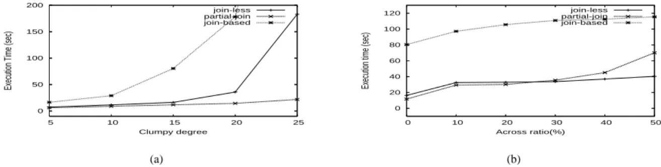
We examined the behavior of the partial join algorithm with the density of neighborhood areas and the cut instances by the explicit partition of spatial data.
1) Effect of data density in neighborhood areas: The density
of neighborhood areas was controlled by lumpy degree
in Fig. 10 (a). The synthetic datasets had around 10% cut neighbor relations by disjoint clique partitioning in the partial join algorithm. The partial join algorithm performed well even if the data density increases withlumpydegree. The reason is
that the points are clustered in some neighborhood areas with fixed cut relations. By contrast, the join-less algorithm shows an increase in execution time with the increase of density. The join-based algorithm always shows higher execution time than the other algorithms.
2) Effect of cut relations: In the second experiment, under
a fixed clumpy degree of 15, we increased the number of cut relations. The number of cut relations is controlled by the aross ratio in synthetic data generation. At lowaross
ratios, the partial join algorithm with fewer cut relations shows
better performance than the join-less algorithm. However, the execution time increases with the increase of thearossratio
because of the increase of inter neighborhood instances and the increase of instance join operations to trace them. Overall, the join-based algorithms increase in execution time with increase of the across ratio due to the increase of neighbor density.
B.4. Evaluation with real datasets
We used two different types of real world datasets. One was an Earth climate dataset related with vegetation growth [16]. Another was an Ecology animal behavior dataset that con-tained chimpanzee observation data from 1999 to 2001 [4].
1) Earth climate data: The earth climate dataset includes
monthly measurements of variables such as global plant growth, e.g., Net Primary Production(NPP), and climate vari-ables, e.g., precipitation(PREC) on latitude-longitude spherical grids. An example of a discovered co-location pattern was (NPP-Hi, PREC-Low), where Hi(Low) denotes an unusually high(low) value of the measurements. The total number of event features was 18. The total number of instances was 15,515. We used 4 as a neighborhood distance, which means 4 cells (each grid cell is 1 degree1 degree). In Fig. 11 (a),
the join-less method shows much better performance at the lower threshold values. The performance difference between the partial join method and the join-based method is relatively small because the cut relation ratio was almost 0.8.
2) Ecology animal behavior data: The animal behavior dataset has 24 chimpanzee features. We assigned a unique instance id to different location points per chimpanzee id. The total number of point instances was 698. Fig. 11 (b) presents