A deep learning approach to sentiment analysis in Turkish

(1)

A Deep Learning Approach to Sentiment

Analysis in Turkish

A thesis submitted to the

Graduate School of Natural and Applied Sciences

by

Basri

_Çİftçİ

in partial fulfillment for the degree of Master of Science

in

(2)

(3)

(4)

“The quieter you become, the more you are able to hear. ”

(5)

A Deep Learning Approach to Sentiment Analysis in Turkish

Basri_Çİftçİ

Abstract

Sentiment analysis is an application of natural language processing (NLP) which is a subfield of artificial intelligence. Sentiment analysis is used to determine the polarity of the thoughts mostly on social media posts, product or different media reviews. Due to its growing demand by data scientists and social media analysts it is one of the most popular topics in NLP. Beside the lexicon-based techniques, from well-known machine learning techniques to advanced algorithms such as deep learning algorithms, there are different kind of algorithms and approaches developed to obtain a good sentiment analysis tool. This study proposes using recurrent neural networks, a type of deep learning algorithm for sentiment analysis in Turkish. Traditional machine learning methods such as logistic regression or Naive Bayes are often applied to this problem however their applicability is limited since they use bag-of-words model which does not take into account the order of the words in a sentence.

In this study we compare these approaches with a modern technique called recurrent neural networks using LSTM units on a dataset crawled from a Turkish movie website. Our results show that RNN based approaches improve the classification accuracies. Keywords: Sentiment analysis, LSTM, RNN, Word vectors, Tf-idf, Deep Learning, NLP, Naive Bayes, Logistic Regression

(6)

Derin Öğrenme Metodları Kullanılarak Türkçe’de Duygusal Analiz

Basri_Çİftçİ

Öz

Duygusal analiz makine öğrenmesinin alt dallarından biri olan doğal dil işlemenin prob-lemlerinden biridir. Çoğunlukla sosyal medya paylaşımlarının, ürün ve medya yorum-larının kutupluluğunu belirlemek için kullanılır. Veri bilimcileri ve sosyal medya analist-lerinin bu konuya olan ilgilerinden ötürü doğal dil işlemenin en popüler konuları arasın-dadır. İyi bir duygu analizi ölçer elde etmek için veri sözlüğü bazlı yöntemlerin yanı sıra, çokça bilinen tekniklerden ileri düzey algoritmalara varıncaya kadar farklı türlerde uygulamalar geliştirilmiştir.

Bu çalışma, Türkçe’de duygu analizini için öğrenme metodlarını önerir. Mantıksal re-gresyon ve Naïve Bayes sınıflandırıcılar gibi geleneksel makine öğrenme metodları bu problemin çözümü için kullanılmaktadır. Fakat kelime kümeleri (bag-of-words) model-lerini kullanan ve kelimelerin cümle içerisindeki yerini gözardı eden bu metodların uygu-lanabilirliği sınırlıdır.

Bu çalışmada, bu bilinen yaklaşımları modern teknikler olarak sayabileceğimiz LSTM gibi Özyinelemeli Sinir Ağlarıyla, filmler hakkında bilgiler içeren popüler bir Türkçe web sitesinden elde ettiğimiz veriseti üzerinde uygulamalar yaparak karşılaştırıyoruz. Sonuçlarımız Özyinelemeli Sinir Ağları’nı kullanan yöntemlerin sınıflandırma sonuçlarında gelişme gösterdiği yönündedir.

Anahtar Sözcükler: Duygusal Analiz, LSTM, Özyinelemeli Sinir Ağları, Kelime Vek-törleri, Tf-idf, Derin Öğrenme, Doğal Dil İşleme, Naive Bayes, Mantıksal Regresyon

(7)

To my family. . .

(8)

Acknowledgments

I would like to thank my thesis advisor, Barış Arslan, for his support and guidance. I owe gratitude to Mehmet Serkan Apaydın, who was my thesis advisor since the be-ginning of this study, for his extreme support, guidance, and valuable advice. Since the very beginning of my journey at this university, he helped me a lot in several courses. I want to thank Burcu Yılmaz for being in my thesis committee, for her time and valuable feedback.

I would like to thank my colleagues and dataLabs team in my company who supported me and shared with me great sources for my thesis. Especially I want to thank my manager Huseyin Ozcan for his support and patience while I was in trouble to find the time to run both my education and work.

I want to thank my dearest friend Reyhan Lütfiye Okumuş for her support and help in linguistics.

Many thanks to my dearest friend Ayşe Semerci for her support and advice whenever I found myself in trouble.

Special thanks to Doğukan Kotan for his early scraping code which helped me a lot to prepare the dataset and to Berk Baytar who helped me to have professional skills of data collection.

I would like to thank my beloved home mates, Alen Lepan and Ahmet Tekin, who supported me a lot, gave me a spot in their home to study even when I was not living with them.

I gratefully acknowledge the support of NVIDIA Corporation with the donation of two Titan Xp GPU’s used for this research.

And, I do not know how to thank my family, for their greatest support, guidance, beliefs, and prayers. I wouldn’t achieve any of my goals without their support.

(9)

List of Figures

1.1 Worldwide search trends on Google for ’Sentiment Analysis’ term for last

ten years. . . 2

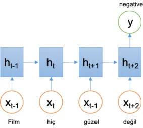
2.1 An example of a sentence fed to an LSTM network with many-to-one architecture . . . 8

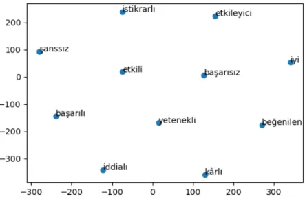
2.2 Word vector representation for a set of words in 2 Dimensions. We use word vectors for sentiment analysis in Turkish using deep learning. . . 11

2.3 Confusion matrix table . . . 12

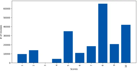
3.1 Raw Dataset characteristics. We have a total of 220066 sentences which are rated between 1 and 10 with a 1, 10 corresponding to the most negative and most positive review, respectively. . . 13

3.2 Positive - neutral - negative distribution. We thresholded the labels such that all sentences with a label of less than 4 were classified negative, more than 6 were classified positive and the rest as neutral. The total number of positive, neutral and negative sentences are 146379, 50053 and 23634 respectively. . . 15

3.3 Overall Dataset characteristics used for the study. The total number of positive and negative sentences are 146379 and 23634 respectively. In total we have 170013 reviews in the dataset. . . 15

4.1 Random oversampling method . . . 19

4.2 Confusion matrix for Naive Bayes with tf-idf vectorizer . . . 20

4.3 Confusion matrix for logistic regression with tf-idf vectorizer . . . 21

4.4 Overview of Word Vectors - RNN application . . . 23

4.5 Accuracy curve of our LSTM model with FastText and Word2Vec, as a function of number of epochs . . . 25

4.6 Loss curve of our LSTM model with FastText and Word2Vec, as a function of number of epochs . . . 25

4.7 Accuracy curve of our LSTM model with FastText, as a function of number of epochs . . . 26

4.8 Loss curve of our LSTM model with FastText, as a function of number of epochs . . . 26

4.9 Accuracy curve of our LSTM model with Word2Vec, as a function of number of epochs . . . 27

4.10 Loss curve of our LSTM model with Word2Vec, as a function of number of epochs . . . 27

4.11 Accuracy curve of unidirectional LSTM models with different hidden lay-ers, as a function of number of epochs . . . 28

(12)

List of Figures xi

4.12 Loss curve of unidirectional LSTM models with different hidden layers, as a function of number of epochs . . . 30 4.13 Accuracy curve of bidirectional LSTM models with different hidden layers,

as a function of number of epochs . . . 30 4.14 Loss curve of bidirectional LSTM models with different hidden layers, as

a function of number of epochs . . . 31 4.15 Accuracy curve of unidirectional and bidirectional LSTM models with 4

hidden layers, as a function of number of epochs . . . 31 4.16 Loss curve of unidirectional and bidirectional LSTM models with 4 hidden

layers, as a function of number of epochs . . . 32 4.17 Accuracy curve of unidirectional GRU models with different hidden layers,

as a function of number of epochs . . . 32 4.18 Loss curve of unidirectional GRU models with different hidden layers, as

a function of number of epochs . . . 33 4.19 Accuracy curve of unidirectional LSTM and GRU models with 4 hidden

layers, as a function of number of epochs . . . 33 4.20 Loss curve of unidirectional LSTM and GRU models with 4 hidden layers,

(13)

List of Tables

3.1 Examples from dataset . . . 14

3.2 Examples of normalization suggestions by Zemberek NLP Library . . . 16

3.3 Most similar words to the word ’kadın’ by FastText . . . 17

4.1 Hyperparameters used in RNN models . . . 22

4.2 Comparison table for baseline methods and 1-layer RNN models . . . 25

4.3 Comparison table for RNN models with different number of layers trained with FastText 300dim word vectors . . . 28

4.4 Elapsed time for training models . . . 31

(14)

Abbreviations

CBOW ContinuousBag of Words CNN Convolutional Neural Network DNN DeepNeuralNetwork

GPU Graphical Processing Unit GRU Gated Recurrent Unit

HTML HyperText MarkupLanguage LSA LatentSemanticAanalysis LSTM Long ShortTerm Memory NLP Natural Language Processing POS Part of Speech

RNN RecurrentNeural Network

RNTN RecursiveNeuralTensor Network SVM Support Vector Machine

TF-IDF TermFrequency - Inverse DocumentFrequency TPU TensorProcessing Unit

(15)

Chapter 1

Introduction

Sentiment analysis is one of the most popular applications in natural language processing (NLP). Many people comment or share their thoughts on ongoing events, politics, things they buy, articles they read or videos they watch online. The opportunity to measure the polarity of thoughts or comments attract the interest of many people, especially marketers, and data engineers. From this perspective, sentiment analysis, which aims to find that polarity, can be considered as a text classification problem and there are many attempts to find a better way to solve this problem in the field.

Figure 1.1 shows the search trends on Google for the last ten years. Clearly the search for the term ’Sentiment Analysis’ has increased on Google over the years. Moreover, by the time of this study the number of GitHub repositories related to ’Sentiment Analysis’ is 18,788 as of March 18, 20191. Therefore, it is obvious that sentiment analysis is a hot topic in natural language processing.

Although in most of the studies, datasets are in English, the topic is not new for languages like Turkish. Well-known machine learning methods such as Naive Bayes and support vector machines (SVM) have already been applied to analyze text in Turkish.

The main motivation behind this study is that deep learning methods have been quite successful in natural language processing tasks such as machine translation and we want to apply those significant novel developments to a newly obtained dataset of reviews in Turkish.

1

https://github.com/search?q=sentiment+analysis

(16)

Chapter 1. Introduction 2

Figure 1.1: Worldwide search trends on Google for ’Sentiment Analysis’ term for last

ten years.

A quick summary of recent developments in NLP using deep learning is as follows: Firstly, word vectors [1, 2] are recently able to convey the meaning of words very ac-curately while representing the words as a vector in a high (such as 300) dimensional space as seen in Figure 2.2. Google and Facebook have their own word vectors with their corresponding dictionaries (the vector representation of every word) available in most languages.

Secondly, deep learning is a very popular machine learning sub-field which has gained significant impact due to the improvements in training algorithms, computational frame-works such as tensorflow [3] and keras [4], and the availability of corresponding hardware such as graphical processing units (GPU’s) or tensor processing units (TPU’s) [5]. In particular, recurrent neural networks allow representing sequential input such as words in a sentence which makes them suitable for NLP applications. One of the most typical applications of such computational frameworks is sentiment analysis.

In this study, our contributions are as follows:

1. We implement preprocessing algorithms in Turkish to prepare sentences to be loaded into sentiment analysis algorithms.

2. We scrape a new dataset in Turkish from online website of movie reviews consisting of 220K sentences.

3. We implement Naive Bayes and logistic regression based algorithms for sentiment analysis as a baseline to compare with our RNN based implementation.

(17)

Chapter 1. Introduction 3

4. We implement RNN based algorithms and compare GRU and LSTM performance results for sentiment analysis.

5. We test our deep learning architecture with varying the number of layers and with both unidirectional and bidirectional architectures.

6. We test and compare these algorithms on this dataset.

In the following chapters, we review the previous work on sentiment analysis approaches in Turkish, the characteristics of the dataset we have obtained for this study, the prepro-cessing steps applied to prepare the dataset, the computational experiments and finally the evaluation and conclusion of the work.

(18)

Chapter 2

Background

Sentiment analysis is a text classification problem which aims to measure the polarity of written documents such as product reviews, news articles, documents that contain opinions, political thoughts, tweets, etc. This polarity is whether the documents reflect a positive or negative, and also sometimes a neutral sentiment. This is useful to deter-mine the popularity of products, movies, and to have an automated analysis of people’s opinions on various subjects. Such an automated tool is invaluable as data is exploding everywhere and it is infeasible to make an analysis of these documents without a reliable software based tool.

Here are some examples where sentiment analysis is important to determine emotional polarity of a sentence. Martin Seligman is one of the important names in modern psy-chology who uses this type of analysis to assess how a person will respond to various positive and negative events in one’s life. He used sentiment analysis techniques in order to assess the comments made by players in various teams and their coaches and to assess their "explanatory styles" which determine how a person explains events in their life to themselves and reflects their feeling of well-being. [6]

A second example of sentiment analysis is done on political opinions of people in election campaigns, and about products by companies in order to manage the perception of voters or product users.

These examples briefly convey the importance of sentiment analysis as a natural language processing tool for data scientists, marketers and even politicians to quickly assess the polarity of people’s opinions on various matters.

(19)

Chapter 2. Background 5

The following sections will describe methods and steps to perform sentiment analy-sis. These are text preprocessing algorithms, classification algorithms based on machine learning that take the preprocessed text and come up with a prediction, and ways to measure the accuracy of a sentiment analysis algorithm. Text vectorizers, lexicon-based approaches and machine learning algorithms are explained below. Then, we list the sig-nificant novel developments in NLP and deep learning approaches to obtain a sentiment analysis tool. Finally, we examine hyperparameter tuning for learning algorithms and metrics to evaluate the results.

2.1 Early Work - Lexicon-based Approaches

The earlier approaches for sentiment analysis are lexicon-based. To use this approach, we need to find the contextual meaning of the words to classify documents. In this regard, there are some studies which categorizes words by doing grammatically parsing operations. This consists of categorizing nouns, verbs, adjectives, adverbs, etc. for a par-ticular language and determining their antonymity or synonymity to find the contextual meaning of the words. Study of Miller et al. results in an English corpus and serves as a library, namely Wordnet [7]. There is a similar study in Turkish which is done by Bilgin et al. [8] and by Dehkharghani et al. [9].

Sentiment analysis with a lexicon based approach then consists of selecting a subset or all of the words in the document and using a library to find the positive or negative words in a text to measure the polarity of the text and classify it accordingly.

In addition, one can use other feature extraction methods to classify the documents such as using part-of-speech tags instead of all words in a document and follow the same logic above, which is mentioned in the study of Hu and Liu [10].

2.2 Machine Learning Approaches

One can also use machine learning based approaches with unlabeled (unsupervised learn-ing) or labeled data (supervised learnlearn-ing) for sentiment analysis.

(20)

As in lexicon based approaches, machine learning based approaches also extract features from the documents to classify them. Generally one can use bag-of-words model to obtain a feature matrix of the documents with the basic machine learning approaches. In this model, single word sequences of the words (unigram) or pairs of words (bigram) or more (n-gram) can be extracted and their frequencies in the whole documents can be determined. For instance, with help of a tf-idf vectorizer, one can find the frequency of the words in the documents to feed them to a machine learning algorithm.

Naive Bayes and logistic regression are two algorithms we examine in this section.

2.2.1 Naive Bayes Method

In Naive Bayes classifiers, each word in a sentence is considered separately and the probability of each word being associated with a positive or a negative sentiment is combined by multiplication to estimate the sentiment associated with the whole sentence. The words in a sentence are assumed to be independent (hence "naive") and the order of the words does not matter. The formal definition of Naive Bayes classifier applied in text classification problems can be stated asPc∈C(x1, x2, ..., xn|c)P(c)whereC is the classes

(either positive or negative),xi is a word in a sentence andP(c)is the prior probability

of class c[11].

2.2.2 Logistic Regression Method

In this classifier, the weighted sum of the sentence features, which are tf-idf vectors in our study, are computed with bias term. The result is fed to a sigmoid function which gives the estimated probability of that sentence being either positive or negative. In a formal way, we can state logistic regression model as σ(θTx+b) whereσ is sigmoid function,θ is a weight matrix andx represents the features [12].

2.2.3 Literature Review

A draft version of Jurafsky’s book [11] includes a section related to sentiment classifica-tion problem. The book, which includes a wide range of topics in NLP, states instrucclassifica-tions to build a sentiment analysis algorithm from scratch and gives an example of using tf-idf

(21)

vectorizer and Naive Bayes classifier. Raschka’s book [13] includes a solution which ap-plies logistic regression classifier on tf-idf scores of IMDB database1, which is a widely used dataset for sentiment analysis in English.

When we look at the studies which are developed for Turkish datasets, we find that the majority of them are using traditional machine learning models. Unlike languages like English, morphologically rich languages like Turkish [14] need custom parsers or stemmers. In morphologically rich languages, sentences contain complex words that are formed by inserting derivational or inflectional morphemes before/after the root. For example, while ’başar-’ is a Turkish verb equivalent to ’to succeed’ in English, you may derive a sentence from that single word with suffixes like ’başarmalıydın’ which can be translated as ’You should have succeeded.’ Another marginal example of a Turkish sentence is ’Çekoslovakyalılaştıramadıklarımızdansınız.’ which can be translated as ’You are among the ones we are not able to convert to someone who is from Czechoslovakia.’. As can be seen, the words either should be morphologically parsed to be handled or should be stemmed to obtain the root word, which may disrupt the meaning of the sentences.

There are different kind of studies that handle the above-mentioned issues for sentiment analysis applications. One of the first sentiment analysis studies in Turkish is done by Erogul in 2009 [15]. He worked on Beyazperde2 movie reviews and grabbed n-grams and part-of-speech (POS) tags as features. In his study, the best accuracy gained by SVM classifier is 85%.

Kaya [16] in 2012 studied sentiment analysis on political news from 6 different newspaper columnists and used continuous bag-of-words (CBOW) framework and n-gram char based language models. Their methodology was using effective words in Turkish, which are strongly as positive or negative, for determining the sentiment of text pieces as labels. With help of different kind of classifiers like Naive Bayes, SVM and Maximum Entropy, they achieved different range of accuracies up to 77%.

Another study conducted by Turkmenoglu [17] was on both scraped Turkish tweets and Beyazperde movie reviews. He used tf-idf vectorizers after preprocessing steps and

1_{http://ai.stanford.edu/ amaas/data/sentiment/} 2

(22)

Figure 2.1: An example of a sentence fed to an LSTM network with many-to-one

architecture

applied SVM, Naive Bayes and Decision Tree classifiers to find the best accuracy, which is obtained by SVM to be 89.5%.

Vural’s study [18] in 2013 on Beyazperde reviews has a different approach with unsuper-vised learning with help of a customized version of Sentistrength [19] library to Turkish. There are also combined methods which uses both lexicon-based and learning-based methods to find sentiment of documents. One of the recent studies on this topic in Turkish was conducted by Gezici [20] in 2018 and her contribution was to combine lexicon based approaches and machine learning methods. She used SentiTurkNet [9] library for polarity lexicon and examined the effect of strong indicators like muhteşem (excellent), negation handling and booster words like çok (very) in sentences. The best accuracy of the study was 75% with SVM classifier.

2.3 Deep Learning Approaches

In this section, we examine enhanced techniques compared to above-mentioned ones for our study. There are different kind of deep learning algorithms for text classification and recurrent neural networks are one of them.

(23)

2.3.1 Recurrent Neural Networks (RNNs)

RNNs are a type of neural network architecture with the ability of holding state infor-mation in addition to producing an output for a given input. This allows them to be applicable to data which has a certain order in them. Some of the most popular individ-ual units in these neural networks are GRUs (Gated Recurrent Units) and LSTMs (Long Short Term Memory Units). These units can be stacked on top of another in order to produce deep RNN architectures. Figure 2.1 shows an example of an LSTM architecture with many-to-one feature which is used for binary classification problems. One challenge in the training of RNNs is the vanishing and/or exploding gradient problem which cor-responds to the backpropagation algorithm updates to the connection weights between the units becoming too small or too large in a deep stacked architecture, thus making it difficult to update the weights of the early layers of the RNN architectures. Methods of overcoming this problem include regularization methods such as dropout [12, 21].

2.3.2 Literature Review

As we mentioned before there are different kind of deep learning methods that can be used to develop a text classification tool. Deep Neural Networks (DNN) which stacks a number of hidden layers can be used for sentiment analysis problems. Recurrent neural networks using LSTMs and GRU’s are also used for sentiment classification [22]. Convolutional neural network (CNN) which are common for image clasification problems is another deep learning algorithm used for sentiment analysis [23, 24].

Not only single algorithms, but also hybrid solutions such as using both CNN and LSTM models together are suggested by Wang [25]. Another example of hybrid algorithms which is the combination of RNNs and CNNs to obtain recurrent convolutional neural networks are proposed in the study of [26].

Recursive models such as recursive neural networks, recurrent tensor neural networks (RNTN), matrix-vector RNNs (MV-RNN) are some other advanced deep learning models which are able to handle the sentences by weighting each node of a parse tree of a sentence. Moreover, they can give different scores to the parts of compound sentences such as sentences includes conjunctions [27].

(24)

2.4 Practical Aspects of Running a Sentiment Analyzer

2.4.1 Preprocessing - Text Vectorizers

Whether we do statistical analysis on text documents or we feed them to machine learning or deep learning algorithms, we should convert the text documents into numeric data to do mathematical operations. In this regard, we process our text documents before feeding them to classifiers by vectorizing them. There are two methods to perform this action that we mention in the following subsections.

2.4.1.1 Tf-idf Vectorization of Sentences

Using term frequency - inverse document frequency (tf-idf) method for text classification is one of the common methods in natural language processing [28]. We use tf-idf to find out the frequency of the words in the document and to weight them with respect to how common or rare these words are.

Tf-idf is a preprocessing method to count the number of occurrences of words in sentences while downweighting very frequent words [13, 29]. The formal definition of tf-idf is as follows: term frequency (tf) is the frequency of a word in sentences and inverse document frequency (idf) is defined aslog(_dfN

i), whereN is the number of sentences, anddfi is the

number of sentences which contains the word i. tf-idf score is the combination of both tf and idf aswij =tfijidfi wherei is a word in a sentencej [11].

2.4.1.2 Word Vector Representation

In many traditional natural language model techniques, words are represented with a one-hot encoding where the index of the word in the dictionary is represented by 1 and the rest of the entries by 0 in the vector. Words of similar meaning do not have similar vector representations with this approach. In contrast, one of the best techniques to represent a word is to encode it on high dimensional space such that words of similar meanings are close in this high dimensional space. Such representations could ideally be learned in an unsupervised manner from a huge amount of text data. Word2vec is an approach based on this idea. In this approach, the word vectors are learned by

(25)

Figure 2.2: Word vector representation for a set of words in 2 Dimensions. We use

word vectors for sentiment analysis in Turkish using deep learning.

associating a word with its context, which consist of the words that surround the word for which one would compute a word vector. There are two methods to compute word vectors in Word2vec. Continuous Bag of words (CBOW) predicts a word based on the context, and the Skip-gram predicts surrounding words given a word. [1]. By training each word in the text data with one of these architectures, similarity among completely different words or words with the same root and different suffixes can be measured. The study of Thomas Mikolov et al. [1] which proposes a way to represent words as high dimensional vectors, namely word vectors, is one of the leading representations and can be used for text classification problems such as sentiment analysis [1].

2.4.2 Hyperparameter Search

One of the obstacles after data preparation and learning algorithm selection is to find the best hyperparameters for training. Machine learning model parameters such as learning rate, the type of regularization that is used, activation and cost functions can vary based on data characteristics and the problem. Hyperparameter Search allows to determine the best hyperparameters by computing the accuracy of a given set of parameters on a validation dataset which is different from the training set, and reporting the best set of hyperparameters. Hyperparameter search can be done on a grid or randomly, depending on the dimension of the parameter space to be searched [12]. Grid Search method tries all combinations of hyperparameters in a methodical way and can be time consuming.

(26)

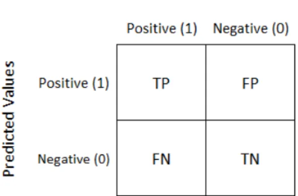
Figure 2.3: Confusion matrix table

2.4.3 Measuring the Accuracy of Sentiment Analysis

After training machine learning models, for evaluation of the accuracy, the number of correct predictions over total predictions can be used over the training and test datasets and the result on the test dataset is reported as the accuracy. In addition, precision and recall are two metrics typically used to evaluate the performance of a sentiment analysis system. Precision or specificity is the accuracy of positive predictions, and recall is the ratio of correctly predicted positive instances. These can be measured by observing the confusion matrix (Figure 2.3) of a trained model [12].

We can simply define the metrics as follows with help of a confusion matrix:

• Accuracy is the number of correct predictions over all prediction result by com-puting(T P +T N)/(T P +F P +F N +T N).

• Precision or Specificityis the positive predictions by computingT P/(T P+F P).

• Recall or Sensitivity is the ratio of correctly predicted positive instances by computingT P/(T P +F N).

(27)

Chapter 3

Dataset

3.1 Data Collection

One of the major problems for machine learning problems is to find a clean and well populated dataset to work on. For many NLP problems there are a number of datasets over the internet. Unfortunately most of these datasets are in English, specifically for sentiment analysis most of the training is done either on IMDB reviews or on scraped tweets. For sentiment analysis in a different language such as Turkish one needs to create their own dataset. For this study, scraped movie reviews from beyazperde1, a Turkish

1_{http://www.beyazperde.com}

Figure 3.1: Raw Dataset characteristics. We have a total of 220066 sentences which are rated between 1 and 10 with a 1, 10 corresponding to the most negative and most

positive review, respectively.

(28)

Chapter 3. Dataset 14

Table 3.1: Examples from dataset

Review Score

Senaryo ve oyunculuklar gayet başarılı ama bana yine de tanımlayamadığım bir şeyler eksik gibi geldi.Yine de iyi diye-bilirim.

8

Tamamen vakit kaybı. Morgan Freeman nasıl olur da böyle vasat bir filmde rol alır anlamak mümkün değil.

2

movie database website were collected. The process of collecting this dataset was done on a PC with 16GB of RAM and 2.2 GHz CPU and it took two days to assemble the dataset.

We have written an algorithm which surfs over the target website for collecting reviews commented for movies. In Beyazperde, a Turkish version of IMDB, users can comment on and rate movies. We scraped all of the movies listed in Beyazperde. We used the reviews as training sentences and converted the ratings to labels. The rating scale is in the range from 1 to 10 where 10 indicates that the user liked the movie very much. Table 3.1 shows examples of two reviews from dataset with their scores.

3.2 Data Characteristics

The total number of reviews in the original dataset is 220066 and all of them are in Turkish. The figure 3.1 shows the number of reviews for each rating score. Since we consider the polarity of sentences, they should be grouped based on their scores. Labels more than 6 were treated as positive, less than 4 as negative and the rest were treated as neutral reviews. Hence, the number of positive, neutral and negative reviews were 146379, 50053 and 23634 respectively. Data distribution after grouping can be seen in Figure 3.2.

Since we examine the polarity of the sentences, for this study we have omitted the reviews that are on gray zone, namely neutral ones. Therefore, we have 23634 negative, 146379 positive. In total the number of reviews is 170013 and we only used these in our experiments. When we look at the final data distribution in in Figure 3.3, we see that majority of the reviews are positive ones. Hence it is an imbalanced dataset.

(29)

Figure 3.2: Positive - neutral - negative distribution. We thresholded the labels such

that all sentences with a label of less than 4 were classified negative, more than 6 were classified positive and the rest as neutral. The total number of positive, neutral and

negative sentences are 146379, 50053 and 23634 respectively.

Figure 3.3: Overall Dataset characteristics used for the study. The total number of

positive and negative sentences are 146379 and 23634 respectively. In total we have 170013 reviews in the dataset.

(30)

Table 3.2: Examples of normalization suggestions by Zemberek NLP Library

Original Text Normalized Text

"izledigim en eglenceli animasyonlardan biriydi bravo"

"izlediğim en eğlenceli animasyonlardan biriydi bravo"

"Ozellikle avuc ici kismi cok hosuma gitti onun disinda cirt cirtli olan baglama kismi felan da cok guzel tam elinizi sariyor tam oturuyor ele. Urunun kaliteside guzel bu fiyata kesinlikle kacirmayin. Bende yo-rumlara bakarak aldim, guvenebilirsiniz"

"özellikle avuç içi kısmı çok hoşuma gitti onun dışında cirit cırtlı olan bağlama kısmı falan da çok güzel tam elinizi sarıyor tam oturuyor ele. ürünün kalitesi de güzel bu fiyata kesinlikle kaçırmayın. bende yo-rumlara bakarak aldım, güvenebilirsiniz."

3.3 Preprocessing Steps

3.3.1 Text Normalization

First, all reviews were cleaned from emoticons and HTML tags. The next step was cleaning our dataset. Since the reviews are from web sources, reviews may include abbreviations, spelling errors, etc. To be able to process text documents, spelling checks and vowel corrections should be applied [30, 31]. To cover all sentences and correcting them manually is quite hard and is a time-consuming task. Thanks to the latest version of a Turkish NLP tool Zemberek [32], we could use the normalization tool which corrects misspelled words, typos, vowel corrections, etc. As an example, two sentences from our dataset are fed to Zemberek and their output are shown in Table 3.2. We used this library and applied all corrections and normalization suggested by this library.

For all experiments applied later on, all sentences were converted to lowercase. Finally, as a feature extraction step, in our experiments, we removed punctuation. In baseline methods we removed stop words but in deep learning method we preserved stop words.

3.3.2 Stemmer

For our baseline methods in Section 5, in which Naive Bayes and logistic regression classifiers are applied, tf-idf vectorizers are used. Since the frequency of a generated word with suffixes will not be high in these methods, we stemmed each word and used the root words. For example, ’kadındır’ and ’kadınına’ are morphologically generated words from the word ’kadın’. To find the occurrences of those generated words in another document is a bit rare. Moreover, tf-idf does not consider any relation among those words, although

(31)

Table 3.3: Most similar words to the word ’kadın’ by FastText

Words Similarity Score ’kadınsın’ 0.759 ’kadınlı’ 0.739 ’kadındır’ 0.731 ’kadınını’ 0.728 ’kadınsız’ 0.723 ’kadınlığı’ 0.721 ’kadındı’ 0.707 ’kadınsı’ 0.700 ’kadınına’ 0.694 ’kadınının’ 0.694

they are derived from the same word. Therefore, with help of stemming, the root word ’kadın’ can be used instead of the generated words from this word. For this study we used a Turkish stemmer library developed by Tuncelli [33].

Contrary to the baseline methods, in our suggested method, which is to use word vectors and RNN architectures, word vectors can find a relation among the words that are generated from the same root. As an example, In table 3.3, the most similar 10 words to ’kadın’ obtained by FastText embedding matrix are listed and as it seen they are semantically close to each other. Nevertheless we fed the documents using stemmer and without stemmer in separate runs. In Chapter 3 we compare the results.

3.3.3 Vectorization of Sentences

3.3.3.1 Tf-idf Vectorizer

For all machine learning problems, inputs should be converted to numerical values. With help of tf-idf scores of the documents, feature extraction step can be completed by ob-taining a sparse matrix conob-taining frequencies of the words in the documents. This type of vectorizer is used for baseline machine learning algorithms such as Naive Bayes and logistic regression. After text normalization and stemming operations, tf-idf scores of the sentences are obtained.

(32)

3.3.3.2 Word Vector Representation

For creating word vector embeddings, we used two different learning algorithms. The first one is Gensim [34], which follows the instructions in Mikolov’s early study [1] about word vector representation. This algorithm is word based and we used skip-gram method for training. With this method, one cannot find a word’s vector which is not in the vocabulary used for training. The second algorithm we used is FastText [2], which follows another study of Mikolov and Bojanowski and it has a character based training strategy. It enhances word vectors with sub-word information and is developed and used by Facebook. Since it is a char-based learning algorithm, a sub-word or morphologically generated words can be represented with this embedding. This means that it can generate a high dimensional vector of a word even if it’s not in its vocabulary.

For both algorithms, we have used Turkish article database of Wikipedia2, and created 2 different word embeddings, which have 100 and 300 dimensions. These word embedding matrices are used in our proposed models.

2

(33)

Chapter 4

Experiments

In all methods, data were split into train, and test samples with a stratified method which means training, validation and test sets are balanced. 80% of the reviews are used for training, and the rest were used for testing phase. Additionally, in all experiments, we performed cross-validation on the 20% of the training set and we report our training, validation and test accuracies.

4.1 Baseline Methods

In this section, we applied methods used in a wide range of earlier studies and we call them as baseline methods. We used bag-of-words model in baseline methods which consist of treating a sentence as a set of words.

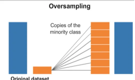
Figure 4.1: Random oversampling method

(34)

Chapter 4. Experiments 20

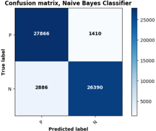
Figure 4.2: Confusion matrix for Naive Bayes with tf-idf vectorizer

4.1.1 Naive Bayes Classifier

After vectorizing documents with tf-idf, the feature vectors were fed to a Naive Bayes classifier. We then did a hyperparameter search in a grid for alpha parameter, which is additive (Laplace / Lidstone) smoothing parameter [35], and we found that best value is 0.1. As can be seen in 3.3, the majority of data is labeled as positive, hence the dataset is imbalanced. To overcome this problem, data oversampling over minority class has been applied. We reused random instances from minority class so that the number of instances in each class became the same. Thus we obtained a balanced dataset. Figure 4.1 shows the method for oversampling. Training time was 7.7 seconds. In Figure 4.2 confusion matrix obtained with Naive Bayes shows our results. Validation and test accuracies, precision and recall scores are 92.7%, 92.9%, 95% and 93% respectively.

4.1.2 Logistic Regression

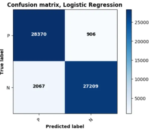
Similar to Naive Bayes method, we vectorized our sentences using tf-idf. We then did hyperparameter search in a grid for regularization (L1 or L2) and C value (a positive float as inverse of regularization strength [35]) and found that best parameters were L2 and 0.2 value of C parameter. We used oversampling as we explained above in Naive Bayes method. Training with this classifier tool 134 seconds. Our results can be seen in Figure 4.3. Validation and test accuracies, precision and recall scores are 94.5%, 94.9%, 97% and 93% respectively.

(35)

Figure 4.3: Confusion matrix for logistic regression with tf-idf vectorizer

Before feeding the instances to these two classifiers, we measured the effect of stemming by preprocessing the words with and without a stemmer. We observe that the results show no significant change on metrics.

4.2 Deep Learning Method

As our main motivation for this study, we apply the novel developments in NLP, more specifically using high dimensional vectors for word representation and deep learning algorithms such as RNNs.

Unlike the previous two methods, with RNNs we do not use tf-idf but instead feed the word vectors directly to the RNN architecture.

After preprocessing steps, as we mentioned in the preprocessing section, we generated 2 embedding matrices that have 100 and 300 dimensions for both FastText and Word2Vec algorithms. In total we obtained 4 different embedding matrices and we used them sep-arately to train our LSTM model. In different runs, we mapped all reviews by those embedding matrices and created a word embedding matrix of the reviews for that par-ticular run. In reviews, the length of the sentence which contains maximum number of words is recorded as ’maximum sequence length’. Based on that, default vector size de-termined. For each word in a sentence, we found the index of that word in the embedding matrix and put them in a row to create a high dimensional vector. For the sentences that have less number of words than ’maximum sentence length’ we filled 0 values to have default vector size. This is called zero-padding. All those high dimensional vectors

(36)

Table 4.1: Hyperparameters used in RNN models

Parameter Value Batch size 64 LSTM unit size 80 Activation Sigmoid Optimizer Adam Learning rate 3e−4 Epoch size 250

Loss Categorical Crossentropy

are concatenated, which becomes a matrix, and those are fed into an RNN architecture using LSTMs or GRUs.

One of the main differences between FastText and Word2Vec is that the former can generate a high dimensional word vector even when the word is not in the model’s vocabulary, because it has a character based learning approach. Unlike the first model, the latter is based on words, so it doesn’t generate a high dimensional word vector for the words which are not in its vocabulary. Therefore when we used Word2Vec, we applied zero padding as well for the words which are not in the vocabulary. Figure 4.4 shows an outline of our methodology.

We applied cross-validation in the training set to report validation accuracies.

To handle the imbalance data problem that we mentioned in baseline methods as well, we reused random sentences from the minority class (negative labelled ones) to have a balanced dataset. Many different combinations of hyperparameters, such as learning rate, batch size, LSTM units size, loss functions and optimizers were tried during training operations to have convergence in both accuracies and loss values.

We list our best hyperparameters in Table 4.1 used in our RNN models after several our tests and trials.

After obtaining best hyperparameters, we increased the number of hidden layers to mea-sure the effects of the complexity of an RNN model for a sentiment analysis. We trained RNNs with up to 4 hidden layers. Moreover, we used bidirectional RNN models to compare them with unidirectional ones. There is also another RNN based architecture besides LSTM, which is called GRU. We also trained our dataset with unidirectional GRUs. We used FastText word vectors with 300 dimensions for these runs.

(37)

(38)

Deep learning models usually require longer training times when compared to the baseline algorithms. We obtained a good performing RNN architecture after 100 epochs. With GPU, it takes 150 minutes to train a bidirectional RNN model with 4 layers while it takes approximately 26 hours with CPUs.

In Figure 4.5 and Figure 4.6 plots of loss and accuracy over number of epochs for our best estimators of unidirectional RNN models with 1 layer, with both Word2Vec and FastText are provided. Although training accuracy tends to increase and training loss tends to decrease in Figure 4.5 and 4.6, we used an early stopping algorithm during our first training attemps, which observes validation loss values to prevent obtaining an overfitting model. Later on, we decided to remove the early stopping algorithm and trained longer and saved the best model after each epoch. We observed the loss values in Figure 4.8 and 4.10 for all runs and reported accuracy and loss values before the corresponding model overfits. Since we ran our algorithm with different embedding matrices, we obtained different training, validation and test accuracies, precision and recall values. The Table 4.2 includes these values. To compare bidirectional and unidirectional RNN models with different number of layers, we also reported training, validation and test accuracies, precision and recall values in Table 4.3.

4.3 Implementation

In our first runs, we used a Macbook Pro with 2.2Ghz CPU and 16GB RAM specifications and the runs took up to more than 26 hours with RNN architecture. Later on, thanks to Titan XP Nvidia GPU’s donated by NVIDIA, we boosted the running time of training our applications. After that the execution time of a training reduced by up to 10x times. We implemented our algorithm in Python with Keras [4] and Scikit-Learn [35] libraries.

4.4 Evaluation

We have experienced different algorithms, methods with different values of hyperparam-eters by tuning several times. Table 4.2 shows the results for the best estimator of each experiment.

(39)

Figure 4.5: Accuracy curve of our LSTM model with FastText and Word2Vec, as a function of number of epochs

Figure 4.6: Loss curve of our LSTM model with FastText and Word2Vec, as a function

of number of epochs

Table 4.2: Comparison table for baseline methods and 1-layer RNN models

Tra. Acc Val Acc Test Acc Precision Recall

N.Bayes w/ tf-idf 92.7% - 92.9% 95% 93%

Log. Regr. w/ tf-idf 94.5% - 94.9% 97% 93%

LSTM-Word2Vec 100D 97.4% 94.3% 94.2% 93% 94%

LSTM-Word2Vec 300D 98.2% 95.4% 95.1% 96% 95%

LSTM-FastText 100D 97.0% 94.6% 94.4% 96% 94%

(40)

Figure 4.7: Accuracy curve of our LSTM model with FastText, as a function of

number of epochs

Figure 4.8: Loss curve of our LSTM model with FastText, as a function of number

(41)

Figure 4.9: Accuracy curve of our LSTM model with Word2Vec, as a function of

number of epochs

Figure 4.10: Loss curve of our LSTM model with Word2Vec, as a function of number

(42)

Table 4.3: Comparison table for RNN models with different number of layers trained

with FastText 300dim word vectors

Tra. Acc Val Acc Test Acc Precision Recall Unidir. LSTM 1-layer 98.1% 95.7% 95.6% 93.9% 97.2% Unidir. LSTM 2-layer 97.6% 95.5% 95.7% 94.8% 96.5% Unidir. LSTM 3-layer 97.1% 95.1% 95.3% 93.2% 97.3% Unidir. LSTM 4-layer 98.1% 95.6% 95.8% 94% 97.7% Bidir. LSTM 1-layer 98.1% 95.6% 95.7% 97.2% 61.2% Bidir. LSTM 2-layer 99% 96.5% 96.6% 97.9% 48.7% Bidir. LSTM 3-layer 99% 96.6% 96.7% 97.7% 77.7% Bidir. LSTM 4-layer 98.5% 96.0% 95.8% 97.4% 77.8% Unidir. GRU 1-layer 97.4% 95.1% 95.1% 94.4% 94.1% Unidir. GRU 2-layer 97.7% 95.7% 95.8% 93.7% 96.4% Unidir. GRU 3-layer 98.2% 95.8% 96% 94.3% 96.6% Unidir. GRU 4-layer 98.5% 95.9% 96.6% 96.5% 87%

Figure 4.11: Accuracy curve of unidirectional LSTM models with different hidden

layers, as a function of number of epochs

When we evaluate the experiment results, we see that among baseline models logistic regression is more successful than Naive Bayes. While applying deep learning methods, we used different word vector encoding algorithms and tested different high dimensional vector sizes. We observe that RNN based models with high dimensional word vectors performed better results over baseline experiments. When we compare Word2Vec and FastText algorithms, we observe that FastText algorithm has higher accuracies than Word2Vec as seen in Figure 4.5 and 4.6. When we observe the Figures 4.7, 4.8, 4.9 and 4.10, we can conclude that 300 dimensional vectors are slightly better than 100 dimensional vectors with both FastText and Word2Vec.

(43)

When we increase the number of hidden layers of unidirectional LSTM architecture, we see that with more layers the model have more stabilized validation and loss graphs and prevents overfitting, as seen in Figure 4.11 and 4.12. Training, validation and test accuracies are better when we increase the number of hidden layers as seen in Table 4.3. When we use bidirectional LSTM models with different number of layers we also see that it converges faster and have better performance if they have more layers as seen in Figure 4.13, 4.14 and Table 4.3. Moreover we compared unidirectional and bidirectional LSTM models with 4 layers and observed that bidirectional models have better loss values and higher accuracies and the latter ones converge faster. The comparision can be seen in Figure 4.15 and 4.16.

We also trained our dataset with RNN based unidirectional GRU architecture and the results show almost similar performance as LSTMs as seen in Figure 4.17 and 4.18. We compared the best unidirectional LSTM model which has 4 layers with the best GRU model which also has 4 layers and results show that for unidirectional RNN models, GRU has better accuracies, loss values and converges faster. The comparison can be seen in Figure 4.19 and 4.20.

For all experiments with unidirectional RNN architecture with one layer, to gain a suc-cessfully converged accuracy and loss graph, the average of time of a training session with deep learning models took approximately 54 minutes of execution. For experiments with RNN architecture which have multilayers or bidirectional ones, training sessions took up to 150 minutes. That means increasing the number of layers of RNN models increases the execution time up to 3 times.

Based on our results, an overall evaluation of our experiments can be summarized as follows:

• Logistic regression with tf-idf has obtained better accuracies than LSTM with 100D word vectors.

• RNN based LSTM with 300D word vectors has sligthly better results than logistic regression and Naive Bayes classifiers for both validation and test accuracies.

• Whether we use unidirectional or bidirectional LSTM models, 2 hidden layers have better convergence and test accuracies than 1 hidden layer. Moreover, there is no need to have more than 2 hidden layers since it increases the execution time and

(44)

Figure 4.12: Loss curve of unidirectional LSTM models with different hidden layers, as a function of number of epochs

Figure 4.13: Accuracy curve of bidirectional LSTM models with different hidden

has no significant change on test accuracies and loss values when we compare 3-4 layered architectures with 2 layered ones.

• Bidirectional RNN models have better performance and accuracy-loss values than unidirectional RNN models.

• GRU has better performance and accuracy-loss values than LSTM models.

• RNNs with 4 hidden layers are 3 times slower than a single layered RNN model.

(45)

Figure 4.14: Loss curve of bidirectional LSTM models with different hidden layers,

as a function of number of epochs

Figure 4.15: Accuracy curve of unidirectional and bidirectional LSTM models with 4 hidden layers, as a function of number of epochs

Table 4.4: Elapsed time for training models

Method Device Elapsed Time

LSTM with word vectors CPU 26 hours LSTM with word vectors GPU 150 minutes Logistic regression with tf-idf CPU 2.2 minutes Naive Bayes with tf-idf CPU 8 seconds

(46)

Figure 4.16: Loss curve of unidirectional and bidirectional LSTM models with 4 hidden layers, as a function of number of epochs

Figure 4.17: Accuracy curve of unidirectional GRU models with different hidden layers, as a function of number of epochs

(47)

Figure 4.18: Loss curve of unidirectional GRU models with different hidden layers,

as a function of number of epochs

Figure 4.19: Accuracy curve of unidirectional LSTM and GRU models with 4 hidden

Figure 4.20: Loss curve of unidirectional LSTM and GRU models with 4 hidden layers, as a function of number of epochs

(48)

Chapter 5

Conclusion

In this study, we examined sentiment analysis in Turkish on a crawled dataset of movie reviews and compared different solutions. First of all we explained how we obtained our dataset and later on analyzed the characteristics of this dataset. We reviewed well known and state-of-the-art approaches in the literature for sentiment analysis. We listed the preprocessing steps and vectorizing methods to prepare text documents before feeding them to learning algorithms. Finally, we compared using recurrent neural networks with word vectors and traditional machine learning approaches such as Naive Bayes and logistic regression with tf-idf vectorizers.

5.1 Discussion

We did sentiment analysis on Turkish movie reviews and while doing this, we applied deep learning methods with high dimensional word vectors. For deep learning architectures we systematically analyzed the parameters. These parameters are whether we should use Word2Vec or FastText, how many hidden layers RNNs should have, whether RNNs should be unidirectional or bidirectional, and whether GRU or LSTM type RNNs should be used. When we analyzed these parameters, we found that the best parameters are bidirectional two layered GRU based RNNs with FastText word vectors. Finally, we compared this method to traditional machine learning algorithms and observed that our proposed method has better performance and results.

(49)

Chapter 5. Conclusion 35

This study is one of the first sentiment analysis studies in Turkish using deep learning methods and high dimensional word vectors and such studies are needed for Turkish. There are some recent related work on this subject such as [36–39].

5.2 Future Work

There are a number of advanced methods in the field which can be examined to have a better solution to this problem. Some of those methods can be listed as using Convo-lutional Neural Networks, using recursive models such as Recursive Neural Networks or Recursive Neural Tensor Network (RNTN) models, hybrid algorithms which are combi-nation of different models [24, 26, 27].

Although it requires much more effort and knowledge of linguistics, there are studies which use parsing methods, negation checks, scoring different parts of compound sen-tences which have conjunctions [27, 40]. They can be the next steps to be taken as future work.

Studies in this thesis may find application areas such as marketing and relevance analy-sis for instance by estimating the relevance of comments made on a site such as ekanaly-siso- eksiso-zluk.com or for estimating the customer interest for a new product.

(50)

Bibliography

[1] T. Mikolov, K. Chen, G. Corrado, and J. Dean. Efficient estimation of word repre-sentations in vector space. arXiv preprint arXiv:1301.3781, 2013.

[2] P. Bojanowski, E. Grave, A. Joulin, and T. Mikolov. Enriching word vectors with subword information. arXiv preprint arXiv:1607.04606, 2016.

[3] M. Abadi, P. Barham, J. Chen, Z. Chen, A. Davis, J. Dean, M. Devin, S. Ghemawat, G. Irving, M. Isard, et al. Tensorflow: a system for large-scale machine learning. In

OSDI, volume 16, pages 265–283, 2016. [4] F. Chollet et al. Keras (2015), 2017.

[5] N. Jouppi. Google supercharges machine learning tasks with tpu custom chip.Google Blog, May, 18, 2016.

[6] M. Seligman. The power of optimism. https://gyroconsulting.com/2014/11/03/

the-power-of-optimism/, 2014. Published: November 03, 2014, Accessed: June

10, 2019.

[7] G. A. Miller. Wordnet: a lexical database for english. Communications of the ACM, 38(11):39–41, 1995.

[8] O. Bilgin, Ö. Çetinoğlu, and K. Oflazer. Building a wordnet for turkish. Romanian Journal of Information Science and Technology, 7(1-2):163–172, 2004.

[9] R. Dehkharghani, Y. Saygin, B. Yanikoglu, and K. Oflazer. Sentiturknet: a turkish polarity lexicon for sentiment analysis. Language Resources and Evaluation, 50(3): 667–685, 2016.

[10] M. Hu and B. Liu. Mining opinion features in customer reviews. InAAAI, volume 4, pages 755–760, 2004.

(51)

Bibliography 37

[11] D. Jurafsky. Speech and Language Processing An Introduction to Natural Language Processing: Computational Linguistics, and Speech Recognition. "Stanford Univer-sity", Draft of August 28, 2017.

[12] A. Géron. Hands-on machine learning with Scikit-Learn and TensorFlow: concepts, tools, and techniques to build intelligent systems. " O’Reilly Media, Inc.", 2017. [13] S. Raschka. Python Machine Learning. Packt Publishing, Birmingham, UK, 2015.

ISBN 1783555130.

[14] R. Tsarfaty, D. Seddah, Y. Goldberg, S. Kübler, M. Candito, J. Foster, Y. Versley, I. Rehbein, and L. Tounsi. Statistical parsing of morphologically rich languages (spmrl): what, how and whither. In Proceedings of the NAACL HLT 2010 First Workshop on Statistical Parsing of Morphologically-Rich Languages, pages 1–12. Association for Computational Linguistics, 2010.

[15] U. Erogul. Sentiment analysis in turkish. Middle East Technical University, Ms Thesis, Computer Engineering, 2009.

[16] M. Kaya, G. Fidan, and I. H. Toroslu. Sentiment analysis of turkish political news. In Proceedings of the The 2012 IEEE/WIC/ACM International Joint Conferences on Web Intelligence and Intelligent Agent Technology-Volume 01, pages 174–180. IEEE Computer Society, 2012.

[17] C. Türkmenoglu and A. C. Tantug. Sentiment analysis in turkish media. In Inter-national Conference on Machine Learning (ICML), 2014.

[18] A. G. Vural, B. B. Cambazoglu, P. Senkul, and Z. O. Tokgoz. A framework for sentiment analysis in turkish: Application to polarity detection of movie reviews in turkish. InComputer and Information Sciences III, pages 437–445. Springer, 2013. [19] M. Thelwall, K. Buckley, G. Paltoglou, D. Cai, and A. Kappas. Sentiment strength detection in short informal text. Journal of the American Society for Information Science and Technology, 61(12):2544–2558, 2010.

[20] G. Gezici and B. Yanıkoğlu. Sentiment analysis in turkish. In Turkish Natural Language Processing, pages 255–271. Springer, 2018.

[21] S. Hochreiter and J. Schmidhuber. Long short-term memory. Neural computation, 9(8):1735–1780, 1997.

(52)

Bibliography 38

[22] Q. T. Ain, M. Ali, A. Riaz, A. Noureen, M. Kamran, B. Hayat, and A. Rehman. Sentiment analysis using deep learning techniques: a review. Int J Adv Comput Sci Appl, 8(6):424, 2017.

[23] C. dos Santos and M. Gatti. Deep convolutional neural networks for sentiment analysis of short texts. In Proceedings of COLING 2014, the 25th International Conference on Computational Linguistics: Technical Papers, pages 69–78, 2014. [24] Y. Kim. Convolutional neural networks for sentence classification. arXiv preprint

arXiv:1408.5882, 2014.

[25] J. Wang, L. Yu, K R. Lai, and X. Zhang. Dimensional sentiment analysis using a regional cnn-lstm model. In Proceedings of the 54th Annual Meeting of the Asso-ciation for Computational Linguistics (Volume 2: Short Papers), volume 2, pages 225–230, 2016.

[26] S. Lai, L. Xu, K. Liu, and J. Zhao. Recurrent convolutional neural networks for text classification. In AAAI, volume 333, pages 2267–2273, 2015.

[27] R. Socher, A. Perelygin, J. Wu, J. Chuang, C. D. Manning, A. Ng, and C. Potts. Recursive deep models for semantic compositionality over a sentiment treebank. In Proceedings of the 2013 conference on empirical methods in natural language processing, pages 1631–1642, 2013.

[28] T. Joachims. A probabilistic analysis of the rocchio algorithm with tfidf for text cat-egorization. Technical report, Carnegie-mellon univ pittsburgh pa dept of computer science, 1996.

[29] J. Ramos et al. Using tf-idf to determine word relevance in document queries. In

Proceedings of the first instructional conference on machine learning, volume 242, pages 133–142, 2003.

[30] R. Dehkharghani, B. Yanikoglu, Y. Saygin, and K. Oflazer. Sentiment analysis in turkish at different granularity levels.Natural Language Engineering, 23(4):535–559, 2017.

[31] K. Adali and booktitle=Proceedings of the 5th Workshop on Language Analysis for Social Media (LASM) pages=53–61 year=2014 Eryiğit, G. Vowel and diacritic restoration for social media texts.

(53)

Bibliography 39

[32] A. A. Akın and M. D. Akın. Zemberek, an open source nlp framework for turkic languages. Structure, 10:1–5, 2007.

[33] O. Tuncelli. Turkish stemmer for python. https://github.com/otuncelli/

turkish-stemmer-python, 2018. Published: October 09, 2018, Accessed: December

29, 2018.

[34] R. Řehůřek and P. Sojka. Software Framework for Topic Modelling with Large Corpora. In Proceedings of the LREC 2010 Workshop on New Challenges for NLP Frameworks, pages 45–50, Valletta, Malta, May 2010. ELRA. http://is.muni.cz/

publication/884893/en.

[35] F. Pedregosa, G. Varoquaux, A. Gramfort, V. Michel, B. Thirion, O. Grisel, M. Blondel, P. Prettenhofer, R. Weiss, V. Dubourg, J. Vanderplas, A. Passos, D. Cournapeau, M. Brucher, M. Perrot, and E. Duchesnay. Scikit-learn: Machine learning in Python. Journal of Machine Learning Research, 12:2825–2830, 2011. [36] M. Kanmaz, E. Sürer, and B. F. Cura. Olumlu mu, olumsuz mu? finansal

haber-lerin anlamsal yönelimi. In2019 Signal Processing and Communication Application Conference (SIU), 2019.

[37] E. B. Dündar and E. Alpaydın. Derin Öğrenme tabanlı yoruma dayalı türkçe haber Özetleme. In 2019 Signal Processing and Communication Application Conference (SIU), 2019.

[38] T. Aytekin, A. Uslu, and S. Tekin. Türkçe film yorumlarında duygu analizi. In2019 Signal Processing and Communication Application Conference (SIU), 2019.

[39] A. A. Karcıoğlu and A. Aydın. Word2vec modelini kullanarak türkçe ve İngilizce twitter mesajlarının duygu analizi. In 2019 Signal Processing and Communication Application Conference (SIU), 2019.

[40] G. Eryiğit, J. Nivre, and K. Oflazer. Dependency parsing of turkish. Computational Linguistics, 34(3):357–389, 2008.

A deep learning approach to sentiment analysis in Turkish

A Deep Learning Approach to Sentiment

Analysis in Turkish

by

Basri

Çİftçİ

A Deep Learning Approach to Sentiment Analysis in Turkish

Abstract

Derin Öğrenme Metodları Kullanılarak Türkçe’de Duygusal Analiz

Öz

To my family. . .

Acknowledgments

Contents

List of Figures

List of Tables

Abbreviations

Chapter 1

Introduction

Chapter 2

Background

2.1

Early Work - Lexicon-based Approaches

2.2

Machine Learning Approaches

2.3

Deep Learning Approaches

2.4

Practical Aspects of Running a Sentiment Analyzer

Chapter 3

Dataset

3.1

Data Collection

3.2

Data Characteristics

3.3

Preprocessing Steps

Chapter 4

Experiments

4.1

Baseline Methods

4.2

Deep Learning Method

4.3

Implementation

4.4

Evaluation

Chapter 5

Conclusion

5.1

Discussion

5.2

Future Work

Bibliography

_Çİftçİ