Housing Price prediction Using Support Vector Regression

(1)

San Jose State University

SJSU ScholarWorks

Master's Projects Master's Theses and Graduate Research

Spring 5-31-2017

Housing Price prediction Using Support Vector

Regression

Jiao Yang Wu San Jose State University

Follow this and additional works at:https://scholarworks.sjsu.edu/etd_projects Part of theArtificial Intelligence and Robotics Commons

This Master's Project is brought to you for free and open access by the Master's Theses and Graduate Research at SJSU ScholarWorks. It has been accepted for inclusion in Master's Projects by an authorized administrator of SJSU ScholarWorks. For more information, please contact

scholarworks@sjsu.edu.

Recommended Citation

Wu, Jiao Yang, "Housing Price prediction Using Support Vector Regression" (2017).Master's Projects. 540. DOI: https://doi.org/10.31979/etd.vpub-6bgs

(2)

& & !&& & !&!&

% & !#& "&

!!&& !$& "&

uyk^Ā Ā ý Ā Ā Ā ²Ā ĀÞĀ Ā Ā Ā $Ā Ā Ā$Ā õĀ Ā ĀĀ ĀĀ

tnj{oĀ !*)&** Jiao Yang Wu

Housing Price prediction Using Support Vector Regression

Digitally signed by Leonard Wesley (SJSU) DN: cn=Leonard Wesley (SJSU), o=San Jose State University, ou, email=Leonard.Wesley@ssu.edu, c=US Date: 2017.05.31 12:32:25 -07'00'

Dr. Leonard Wesley

Robert Chun

Digitally signed by Robert Chun

DN: cn=Robert Chun, o=San Jose State University, ou=Computer Science, email=robert.chun@sjsu.edu, c=US

Date: 2017.05.19 17:58:48 -07'00'

05/19/2017

Dr. Robert Chun

James Casaletto

Digitally signed by James Casaletto Date: 2017.05.20 11:18:41 -07'00'

05/31/2017

05/20/2017

Mr. James Casaletto

(3)

Page 1 of 56

Housing Price Prediction Using Support Vector

Regression

A Project Report 

Presented to 

The Department of Computer Science San Jose State University

In Partial Fulfillment 

of the Requirements for the Computer Science Degree

by Jiaoyang Wu

(4)

Page 2 of 56

(5)

Page 3 of 56

The Designated Project Report Committee Approves the Project Report Titled Housing Price Prediction Using Support Vector Regression

by Jiaoyang Wu

APPROVED FOR THE DEPARTMENT OF COMPUTER SCIENCE SAN JOSE STATE UNIVERSITY

May 2017

Dr. Leonard Wesley Signature: ______________________________ Department of Computer Science

Dr. Robert Chun Signature: ______________________________ Department of Computer Science

Mr. James Casaletto Signature: ______________________________ Department of Computer Science

(6)

Page 4 of 56

Abstract

The relationship between house prices and the economy is an important motivating factor for predicting house prices. Housing price trends are not only the concern of buyers and sellers, but it also indicates the current economic situation. Therefore, it is important to predict housing prices without bias to help both the buyers and sellers make their decisions. This project uses an open source dataset, which include 20 explanatory features and 21,613 entries of housing sales in King County, USA. We compare different feature selection methods and feature extraction algorithm with Support Vector

Regression (SVR) to predict the house prices in King County, USA. The feature selection methods used in the experiments include Recursive Feature Elimination (RFE), Lasso, Ridge, and Random Forest Selector. The feature extraction method in this work is Principal Component Analysis (PCA). After applying different feature reduction methods, a regression model using SVR was built. With log transformation, feature reduction, and parameter tuning, the price prediction accuracy increased from 0.65 to 0.86. The lowest MSE is 0.04. The experimental results show there is no difference in performance between PCA-SVR and feature selections-SVR in predicting housing prices in King County, USA. The benefit of applying feature reductions is that it helps us to pick the more important features, so we will not over-fit the model with too many features.

(7)

Page 5 of 56

Acknowledgements

I would like to thank for my advisor Dr. Lenoard Wesley for his guidance, suggestions, and patience toward my project.

I also would to thank my committee members Dr. Robert Chun and Mr. James Casletto for their feedbacks and supports toward my project.

(8)

Page 6 of 56

List Of Figures

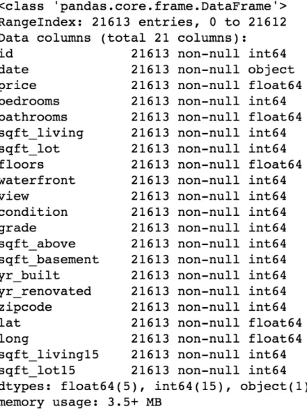
Figure 1: Data information... 19

Figure 2: missing value count ... 20

Figure 3: plots on a selection of features ... 22

Figure 4: Housing price distribution ... 23

Figure 5: price statistics before log transformation ... 23

Figure 6: price statistics after log transformation ... 24

Figure 7: correlation heatmap between features ... 25

Figure 8: standardize features ... 27

Figure 9: transform features ... 27

Figure 10: principal components ... 27

Figure 11: PCA ... 28

Figure 12: covariance matrix ... 28

Figure 13: explained variance ... 29

Figure 14: variance explained plot ... 29

Figure 15: principal components explained in percentage ... 30

Figure 16: MSE plot of different principal components in train data ... 31

Figure 17: MSE plot for different principal components in test data ... 31

Figure 18: MSE for both training and testing data at different PCs ... 32

Figure 19: feature selection results ... 33

Figure 20: sklearn RFE ... 34

Figure 21: RFE ... 35

Figure 22: lasso features ... 36

Figure 23: Ridge features ... 37

Figure 24: Random ForestRegressor() ... 38

Figure 25: Random Forest features ... 38

Figure 26: SVR objective function ... 39

Figure 27: epsilon loss function ... 39

Figure 28: sklearn SVR() ... 40

Figure 29: non-linear separable ... 40

Figure 30: SVR poly kernel ... 41

Figure 31: SVR RBF kernel ... 41

Figure 32: SVR kernels ... 41

(10)

Page 8 of 56

List of Tables

Table 1: data descriptions ... 17

Table 2: data statistics overview ... 21

Table 3: SVR results ... 44

Table 4: SVR with PCA results ... 45

Table 5: SVR with feature selection results ... 46

Table 6:after log transformation results ... 48

Table 7: after log transformation (with PCA) ... 49

(11)

Page 9 of 56

Introduction

The relationship between house prices and the economy is an important motivating factor for predicting house prices (Pow, Janulewicz, & Liu, 2014). There is no accurate measure of house prices (Pow, Janulewicz, & Liu, 2014). A property’s value is important in real estate transactions. House prices trends are not only the concerns for buyers and sellers, but they also indicate the current economic situations. Therefore, it is important to predict the house prices without bias to help both buyers and sellers make their decisions.

There are different machine learning algorithms to predict the house prices. This project will use Support Vector Regression (SVR) to predict house prices in King

County, USA. The motivation for choosing SVR algorithm is it can accurately predict the trends when the underlying processes are non-linear and non-stationary.

There are many factors affect house prices, such as numbers of bedrooms and bathrooms. In addition, choosing different combinations of parameters in Support Vector Regression will also affect the predictions greatly. This project is guided by these

questions: Which features are important for predicting price of houses? How to select those features in the data to achieve a better performance? Which parameters in SVR have better performance in predicting house price? The structure of this report will follow the graph in Fig. 1.

(12)

Page 10 of 56

Fig. 1. Flow of the report

Conclusion and Future Work Results and Discussions

Evaluation Metrics Results Discussions

Methods

Feature Extractions Feature Selections SVR

Data Analysis Data

Data Analysis

Experimental Design

Research Objective and Hypotheses Literature Review

(13)

Page 11 of 56

Literature Review

Support Vector Machine (SVM) was introduced in 1992 by Boser, Guyon, and Vapnik (Boser, Guyon, &Vapnik, 1992). It became popular after its success in handwriting recognition (Bottou et al., 1994). The algorithm was developed from Statistical Learning Theory in 1960s, which is the mathematical foundation of SVM. It gives the conditions for a learning algorithm to generalize effectively (Vert, 2002). There are a range of fields using SVM, such as machine learning, optimization, statistics, and functional analysis. SVM is treated as an important example of kernel methods, which is the key area in machine learning (Martin, 2012). SVM tries to classify objects with large confidence to prevent over fitting, so programmer will avoid fitting too much lines on the training set, which will degrade the performance of generalization (Vert, 2002). A version of SVM called Support Vector Regression was proposed in 1996 by Vapnik and his coworkers (Drucker, 1997).

Pow states that Real Estate property prices are linked with economy (Pow, Janulewicz, & Liu, 2014). He also states there is no accurate measure of house prices. A property’s value is important in real estate transactions. Pow tries to predict the sold and asking prices of real estate values without bias to help both buyers and sellers make their decisions. He analyzes and predicts the real estate property prices in Montreal based on 130 features such as geographical location and room numbers. He compares different machine learning methods such as linear regression, Support Vector Regression, k-Nearest Neighbor, and Random Forest. He concludes that Random Forest outperforms other algorithms (Pow, Janulewicz, & Liu, 2014).

Pow uses dataset consisted of 130 features from Centris.ca and deProprio.com (Pow, Janulewicz, & Liu, 2014). He first pre-processes the data. He determines the outlier by looking at distribution of values. Then he applies feature engineering on the dataset by reducing the dimensionality with Principal Component Analysis (PCA). Pow uses average error as the evaluation metrics. The result is not improved with combining PCA and KNN Algorithm. He uses 10-fold cross validations to train Random Forest model. When increasing the number of trees, the average error decreases to around 0.113.

(14)

Page 12 of 56

Even though KNN has low error (0.1103), it strongly depends on geographical distances between neighbors. (Pow, Janulewicz, & Liu, 2014).

Park’s paper analyzes the housing data on 5359 townhouses in Firfax County, Virgina based on different machine learning algorithms such as RIPPER (Repeated Incremental Pruning to Produce Error Reduction), Naïve Bayes, AdaBoost. He proposes an improved prediction model to help sellers make their decisions on the house price valuations. He concludes RIPPER algorithm outperforms other models on predicting house price (Park & Bae, 2015).

Housing market is growing rapidly and therefore it is hard to predict the house prices. According to Kumar, house price is concern for both individuals and government because house price is a factor of influencing the socio-economic conditions. Kumar tries to find a machine learning approach to predict house prices around Bangalor based on features such as house size and bedroom number. He extracts data from real estate website and analyzes using the dataset with WEKA. Kumar experiments with different machine learning algorithms such as Linear regression, Decision Tree, and Nearest Neighbor (Kumar et al., 2015). He concludes that Naïve Bayes is consistent for unequal distribution frequency and Decision Tree is the most consistent classifier for equal frequency distributions. The error in linear regression is little high, but it predicts numerical values of selling prices instead of a range of selling prices as the other classifiers do (Kumar et al., 2015).

Housing market is important for economical activities (Khamis & Kamarudin, 2014). Traditional housing price prediction is based on cost and sale price comparison. So, there is a need for building a model to efficiently predict the house price. Khamis compares the performance of predict house price between Multiple Linear Regression model and Neural Network model in New York. The dataset is a sample of randomly chosen 1047 houses with features such as lot size and house ages from Math10 website. (Khamis & Kamarudin, 2014). The experimental results show that R square value in Neural Network model is higher than Multiple Linear Regression mode by approximately 27% (Khamis & Kamarudin, 2014). The Mean Squared Error (MSE) in Neural Network is lower than Multiple Linear Regression model. Khamis concludes that Neural Network

(15)

Page 13 of 56

Model has an overall better performance and is preferred over Multiple Linear Regression model (Khamis & Kamarudin, 2014).

Bahia collects the data from UCI Machine Learning Repository. He pre-processes the data, follows by feature selection and transformation. The dataset has 506 samples. Bahia selects 13 variables to use for Artificial Neural Network predictions. He compares the results between Feed Forward Back Propagation Artificial Neural Network with Cascade Forward Back Propagation Neural Network. The input layer is a 13 x 506 matrix, and the output layer is a 1 x 506 matrix of median value of owner-occupied homes (Bahia, 2013). He uses mean square error (MSE) from the output in training, validation, and test as the evaluation metrics. He divides the dataset to 80% training and 20% for testing, and trains up to 100 epochs. Bahia concludes that Cascade Forward Neural Network outperforms Feed Forward Neural Network because the MSE for Cascade Feedforward Back Propagation is less than Feed Forward Back Propagation neural network (Bahia, 2013).

(16)

Page 14 of 56

Research Objective and Hypotheses

Research Objective

In the literature review, we have seen different the results of different machine learning algorithms on house price predictions. They all focus on the results of different machine learning algorithms. There have not been comparisons between the performance of feature selections with SVR and PCA with SVR on house price predictions in King County of USA. Some of the previous work do not involve enough evaluation metrics to help assess and compare the performance of different models. It is important to choose the correct evaluation metrics to test the results. Due to these technical gaps, this project will bridge these gaps by perform comparative study between feature selections with SVR and feature extraction with SVR. The chosen evaluation metrics are R square score, MAE, MSE, and RMSE.

Hypotheses

Alternative hypothesis I : Using Feature Selection techniques will allow Support Vector Regression to have over 5 % lower RMSE than using feature extraction algorithm in PCA with SVR.

Null hypothesis I: Using Feature Selection techniques will not allow Support Vector Regression to have over 5 % lower RMSE than using feature extraction algorithm in PCA with SVR.

Alternative hypothesis II : Using Feature Selection techniques will allow Support Vector Regression to have over 5 % higher R square score than using feature extraction

algorithm in PCA with SVR.

Null hypothesis II: Using Feature Selection techniques will not allow Support Vector Regression to have over 5 % higher R square score than using feature extraction algorithm in PCA with SVR.

(17)

Page 15 of 56

Experimental Design

The experiment compares the results on feature selection techniques with SVR and feature extraction algorithm with SVR. The goal of the experiment is to test the two hypotheses stated above. The experiment has two phase. First phase is reduce the dimension with PCA on the raw features, then use the reduced features as an input for SVR model. Second phase is selected features using different feature selection

techniques, then use the selected feature to carry out SVR model. The chosen evaluation metrics are R square score, Mean Absolute Error (MAE), Mean Square Error (MSE), Root Mean Square Error (RMSE). The steps of the experiment are the followings: Phase 1: Feature extraction using PCA with SVR

1. Use PCA to reduce the dimensionality of the data.

2. Pick the principal components that will generate the lowest MSE error. 3. Use the reduced dimensional features as inputs for the SVR model. 4. Calculate R square score, MAE, MSE, RMSE for PCA-SVR.

Note: The dataset is not square matrix. There are more rows of data than the features. Singular Value Decomposition will be automatically used when calling PCA in scikit-learn library.

Phase 2: Feature Selections with SVR

1. Perform feature selection techniques (RFE, Lasso, Ridge, Random Forest Selectors) to get the important features.

2. Take the mean of the applied feature section technique results, and select the important features.

3. Use the selected features as inputs for the SVR model.

4. Calculate R square score, MAE, MSE, RMSE for feature selections with SVR.

(18)

Page 16 of 56

Data

The dataset for some of the previous works on housing price predictions is not large. For example, Bahia only studies 506 samples to develop the model (Bahia , 2013). There is a limitation in the paper by Pow saying the research does not have enough historical transaction data. Pow points out using enough data might increase the performance of predictions (Pow, Janulewicz, & Liu, 2014).

This project uses a dataset from Kaggle open source datasets. The dataset consists of 20 explanatory features and 21,613 entries of housing sales in King County, USA. It describes different aspects of housing sales from May 2014 to May 2015 (Kaggle Inc.). The table below shows the feature names and their descriptions.

(19)

Page 17 of 56 Table 1: data descriptions

King County is a county in US of Washington. The population is approximately 2,117,125 in July 2015, which is also the County with most population in Washington

(20)

Page 18 of 56

(Census, 2016). There are 893,157 housing units as in July 2015. The median income is $81916 (Datausa).

From the table shown above, we can see the independent variables from the housing dataset are the explanatory variables. The independent variables are date, price, bedrooms, bathrooms, sqft_living, sqft_lot, floors, waterfront, view, condition, grade, sqft_above,sqft_basement, yr_built, yr_renovated, zipcode, latitude, longitude, sqft_living15, and sqft_lot15. We can see that these variables include categorical variables, numerical variables, and time series variables. The dependent variable is the sale price of houses from May 2014 to May 2015 in King County USA.

(21)

Page 19 of 56

There are 21613 observations of house sales price from King County USA in a one year time frame with different aspects. In the figure below, we can see the data does not have any missing values.

(22)

Page 20 of 56

Figure 2: missing value count

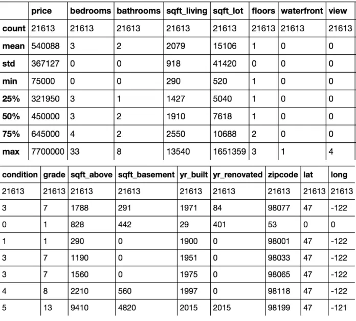
The following table shows the statistics for all the features. There are 21,613 records of data. The average house price is $540,088. The standard deviation of price is 367,127, which is relatively high. The minimum price is $75,000 and the highest price is $7,700,000. In the bedroom number column, we can see that the highest bedroom number is 33, which implies that outliers exist in this column because the average bedroom size is only 3. Also, the maximum lot size is 1,651,359, but the average is only 15,106, which also implies outliers exist for lot size feature. Values that are three

(23)

Page 21 of 56

Table 2: data statistics overview

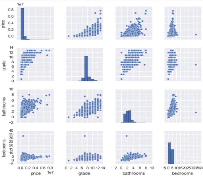
To see the outliers visually, we can use the Seaborn library for Python to draw different plots. The following figure shows the plot on a selection of features: price, grade, bathrooms, and bedrooms. We can see clearly, there exist one or more outliers in these features. In addition, we can see the general trends for price over different features. Most are not very linearly related. Hence, more feature engineer work need to process the data.

(24)

Page 22 of 56

Figure 3: plots on a selection of features

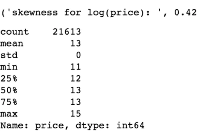
The following figure shows the distribution of the house prices. The plot is clearly shown that the distribution is skewed to the left. To be more precise, the skewness is 4.023, which is very high. A highly skewed data will affect the prediction result greatly. We first apply SVR without log transformation of sale price, the result is not very good. To improve the results, we apply log transformation on the house price to reduce the skewness. After transform the price with log, the skewness reduced to only 0.428. The performance of SVR model also improves, as we will show in the next sections.

(25)

Page 23 of 56

Figure 4: Housing price distribution

(26)

Page 24 of 56

Figure 6: price statistics after log transformation

The following figure shows the correlation matrix heatmap with Python Seaborn library. We can see that there are a few variables have quite high correlated between each other. The correlation between sqft_above and sqft_living is 0.88. The correlation

between sqft_livng and grade is 0.76. In general, the correlation for sqft_living associated features are higher than others. High correlation between features might have

multicollinearity problem. Also, when applying the PCA in the later, it will put larger weight on the features that have highly correlated variables. Therefore, to solve this problem, we can either drop sqft_living or combine sqft_living with sqft_above to create a new feature called sqft.

(27)

Page 25 of 56

Figure 7: correlation heatmap between features

After an overview on the data by visualization and statistical analysis, we have a better knowledge on the data. The next section will discuss how to use PCA to reduce the feature dimensions before serving as an input for SVR model.

(28)

Page 26 of 56

Methods

Feature Extraction with SVR

Principal Component Analysis (PCA)

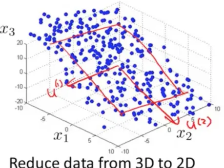
The goal of Principal Component Analysis (PCA) is reduce the dimensionality of data that contains variables with correlation between each other, while maintaining the variation of the data, to the maximum extent (Deyzre). The variables that have lower variance, which are not spread out a lot, will be projected to a lower dimension. Then, the model will be trained on this transformed data.

The PCA in our experiment is implemented by scikit-learn library. Sklearn uses Singular Value Decomposition (SVD) to implement the dimension reduction of PCA. Since our data is not a square matrix, SVD will be automatically applied when we call PCA() from sklearn library. The general steps of PCA are shown as follow:

1. Normalize data

2. Calculate covariance matrix and get the eigenvalues and eigenvectors 3. Choosing principal components and forming feature vector

4. Transform original dataset to get the k-dimensional feature subspace First, we standardize the features. This is a requirement of PCA techniques (Dezyre). We scale the features with Standarscaler() function from sklearn.preprocessing library in Python. Sklearn has different methods to scale the data. Standardscalar() scales all the features to the unit variance (Sklearn). Standardize the data before applying machine learning models is a very common requirement. The accuracy might be low if the data is very skewed to the left or right without standardization. There is one

assumption about the objective function’s elements in SVM RBF kernel : the variables are centered at zero and variance to be in same order (Sklearn). If it contains features with variance that are not in same order, then those features with larger magnitude variance will dominate the objective function; the model will not be accurately predict the data (Sklearn).

(29)

Page 27 of 56

Figure 8: standardize features

Then, use PCA() from Python scikit-learn library to fit and transform the features and get principal components. The following figure shows how to get the principal components after the transformation of the features. The principal components are just the new set of features after transforming them.

Figure 9: transform features

Figure 10: principal components

The following figure shows the covariance matrix of the features (Udacity). Covariance matrix is (1/n) * (M transposed) * (M). The ideal case is the non-diagonal values in the covariance matrix are all zeros. The first principal component is to the direction that has most variance. The second one is the orthogonal vector of the first one. Orthogonal means that the vectors are perpendicular with each other, the dot product mean is zero. There is no covariance between them.

(30)

Page 28 of 56 Figure 11: PCA

Figure 12: covariance matrix

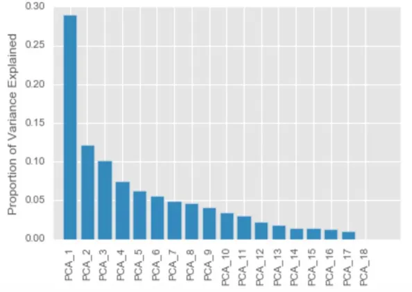
The following three figures show how much variance the principal components explained in ratio and in plot. The first three principal components have about 50% variance explained. Principal components four to nine have about 35% variance

explained. There are two ways to choose the number of principal components. The first way is pick principal components explain most of the variation. The second way is pick principal components that will have a lower error rate.

(31)

Page 29 of 56

Figure 13: explained variance

(32)

Page 30 of 56

Figure 15: principal components explained in percentage

Since one of the goals of this project is to decrease the prediction error rates. So, we choose the second way to pick the principal component numbers. We calculate the lowest mean square error (MSE) for every principal component. The following two figure show the plots of the MSE for eighteen principal components for training data and for testing data, respectively. The lowest MSE in the training data is at sixteen principal components, with MSE equal to 45930386781.5. The lowest MSE for testing data is also at sixteen principal components, with MSE equal to 53895288367.4.

(33)

Page 31 of 56

Figure 16: MSE plot of different principal components in train data

(34)

Page 32 of 56

To compare the MSE between training data and testing data, the following plot is drawn. The MSE for training data is lower at every principal component. The MSE decreases dramatically until principal components equal to seven. After seventh principal components, the MSE for both training data and testing data still decrease, but not a lot.

Figure 18: MSE for both training and testing data at different PCs

We set the principal components equal to sixteen. We choose sixteen instead of seven principal components because we try to minimize the error as much as possible. After transform and fit the data, the transformed features will serve as the inputs for Support Vector Regression. The procedure for SVR will be discussed in the later SVR sections.

(35)

Page 33 of 56

Feature Selections

Since the feature selection methods are not stable, we apply four different feature selection methods. After applying all four methods to the initial set of features, we take the mean of those results. We plot the features with the highest score to the lowest score in the following plot. In the plot, we can see the features with lowest scores are ‘sqft_lot’, ‘sqft_lot15’, and ‘yr_renovated’. It is surprising to see both ‘sqft_lot’ and ‘sqft_lot15’ are not having high score. The following subsections will show how each feature selection technique is used and the result of each feature selection technique.

(36)

Page 34 of 56

Recursive Feature Elimination

Recursive Feature Elimination (RFE) uses an estimator model to rank the features. RFE selects the good features by recursively calling the smaller set of features (Sklearn). Sklearn has built in function to apply RFE to select features. A model need to trained before applying RFE. First, a chosen model is trained on initial set of features. Each feature will be assigned to a weight in the first round. In the second round, the feature with smallest weight will be pruned from the initial set. It will recursively perform this process until the desired number of features is reached (Sklearn). There are different parameters can be specified in RFE functions, as shown in the following figure (Sklearn). The estimator is the chosen supervised model to fit the features. The parameter n_features_to_select is the desired feature we want. If we do not stated this, half feature will be selected from the original set of features.

Figure 20: sklearn RFE

We have tried both SVR (kernel = ‘linear’) and regular linear model as the estimator model. SVR takes a lot longer to train than linear model, but the results of feature importance are same. After training with an estimator model, we call RFE() function to fit the features with the target variable. The figure below shows the result of RFE feature selection. Longitude variables gets assign to a score of zero.

(37)

Page 35 of 56 Figure 21: RFE

Lasso and Ridge

Both Lasso and Ridge use the concepts of coefficients of Regression model to rank the feature importance. The higher the coefficients, the more important the features. Both work well when data is in linear shape and not too many noisy data exist. Since our data do not have many noisy data exist, we assume the Lasso and Ridge will work good. Lasso and Ridge are regularization models. Lasso is L1 Regularization. It adds penalty to the loss function with a term α∑|wi|. The weak features have zero coefficients in Lasso model. Increase alpha parameter in Lasso function will produce more zeros in the coefficient. The following figure shows how we call lasso and the results of the

coefficients. The following variables have zero coefficients: sqft_above, sqft_basement, sqft_living, sqft_15, sqft_lot, sqft_lot15, yr_renovated, and zipcode.

(38)

Page 36 of 56 Figure 22: lasso features

Ridge is a L2 Regularization. It adds penalty to the loss function with a

term α∑|wi|^2. Ridge regularization gives more penalty because the term is the square of the Lasso penalty term. The coefficients spread out more equally than Lasso. It is also more stable than Lasso. The following figure shows how we call ridge regression and the results of their coefficients. The following variables have zero coefficients: sqft_above, sqft_basement, sqft_living, sqft_15, sqft_lot, sqft_lot15, yr_renovated, and zipcode.

(39)

Page 37 of 56 Figure 23: Ridge features

Random Forest Selector

Random Forest is an algorithm built with many decision trees. Every node is a feature condition. Sklearn has RandomForestRegressor() with built in feature importance function. After fitting with RandomForestRegressor(), we can call feature_importances to get the importance score for every feature. The higher the score, the more important the feature is.

(40)

Page 38 of 56

Figure 24: Random ForestRegressor()

(41)

Page 39 of 56

Support Vector Regression

The objective function is a function combining a loss function and flatness (SVR mini-lectures).

Figure 26: SVR objective function

The loss function can be any loss function. Most used loss function is epsilon-insensitive loss function because it is more epsilon-insensitive to a bad data point (SVR mini-lectures). The following figure shows that there is no penalty between the epsilon values. Flatness is the measure of curvature with ith shape function (SVR mini-lectures). One example of flatness function is 𝐹 = 𝜅 𝑏 . We try to minimize the loss function and flatness of the curve.

(42)

Page 40 of 56

We use Python scikit-learn library to build SVR model. There are different parameters in SVR. This project will compare the results between different kernels, C values, epsilon values.

Figure 28: sklearn SVR()

Figure 29: non-linear separable

If the data point is not linear separable, we can use a kernel trick to transform the data. An example of non-linearly data point shown in the above figure (Udacity). The original data will transform to a higher dimensional data so the points can be linear separable. The options of kernels in SVR are linear, poly, RBF, sigmoid, and precomputed (Sklearn). The default kernel is RBF. Choosing the right kernel is very important. R square score can be dramatically affect with different choices of kernel. The two most popular non-linear kernels are polynomial kernel and radial basis function (RBF) kernel. Polynomial kernel is 𝐾(𝑥, 𝑦) = (𝑥 y+1) . RBF kernel is 𝐾(𝑥, 𝑦) =

exp (− ‖𝑥 − 𝑦‖ ). The following figures show the plots for examples of polynomial

(43)

Page 41 of 56

Figure 30: SVR poly kernel

Figure 31: SVR RBF kernel

(44)

Page 42 of 56

The SVR kernels figure shows a comparison with applying different kernels on same dataset (Sklearn). The trend of data follows RBF kernel. If we fit with a wrong kernel such as linear kernel, the model will be under fitted. The model does not capture the trend of the data. Under fitting the model will produce high error and low R square score.

Another important parameter is ‘C’. C is the penalty term. It is a tradeoff between misclassification of training examples and simplicity of the decision surface (Udacity). A lower C has a smoother decision surface. A higher C tries to classify all training data correctly by giving the model more options to choose support vectors.

Epsilon is the epsilon in the epsilon tube. No penalty is associated in the training loss function when points are inside epsilon tube (SVR mini-lectures). The following figure shows the epsilon tube (SVR mini-lectures). The goal is to get as many points fitted within this epsilon tube as possible.

(45)

Page 43 of 56

Results and Discussions

Evaluation Metrics

This project uses four different evaluation metrics to test the hypotheses: R square score, MAE, MSE, RMSE.

R square is the goodness of fit of the predictions to actual values (Coefficient of determination). It is the explained variation divided by the total variation.

MAE (Mean Absolute Error) measures how close the predictions to the actual value. It is the average of the sum of the absolute difference between the predicted value and true value (Metrics).

MSE (Mean Square Error is the average of the error. It is the average of the sum of the squares of the difference between the predicted value and true value (Metrics).

RMSE (Root Mean Square Error) is the square root of the average of all the error. It is simply the square root of the mean square error (Metrics).

(46)

Page 44 of 56

SVR results without feature reductions

The following table shows the R square scores and different test error rates for SVR without any feature reductions. With applying SVR regression model on the initial set of features (exclude id and date), SVR model with linear kernel and C sets to 1000 has the highest R-square score, 0.65. All three error rates are lowest with using linear SVR. Therefore, without performing feature reductions, SVR (kernel = ‘linear’, C =1000) has the lowest RMSE at 231,135.68 and highest R square score at 0.65.

Table 3: SVR results

Kernel C R-square MAE MSE RMSE

Linear 10 0.49 138928.75 137645952853.92 278,480.76 Linear 100 0.62 120969.32 77551535678.49 238,137.81 Linear 1000 0.65 119740.90 56709617656.39 231,135.68 Poly 10 0.16 213886.9 127282458766.08 356,766.67 Poly 100 0.21 178572.01 119825660031.39 346,158.43 Poly 1000 0.51 141816.28 74071135395.94 272,160.13 RBF 10 -0.04 224819.67 157679652596.13 397,088.97 RBF 100 0.09 191570.64 136879612004.73 369,972.45 RBF 1000 0.33 140966.29 101363622894.39 318,376.54

(47)

Page 45 of 56

SVR results with feature extraction using PCA

The following table shows the R square scores and different test error rates for first extract features using PCA and then apply SVR to train the model. After applying SVR regression model on the extracted features with sixteen principal components, the results show that SVR model with linear kernel and C sets to 1000 has the highest R-square score, 0.64. This combination of parameters (kernel = ‘linear’, C = 1000) is same as without feature reductions in the previous table. All three error rates are lowest with using linear SVR. Even the error rates decrease after applying PCA, the R-square score is 0.01 lower than before. Therefore, SVR (kernel = ‘linear’, C =1000) has the lowest RMSE at 226,800.30 and highest R-square score at 0.64.

Table 4: SVR with PCA results

Linear 10 0.47 141220.17 76911305047.56 277328.88 Linear 100 0.62 121462.19 54766443417.89 234022.31 Linear 1000 0.64 120303.78 51438377107.2 226800.30 Poly 10 0.16 210104.24 120804966395.84 347570.09 Poly 100 0.29 173611.51 101944271679.71 319287.13 Poly 1000 0.59 136145.06 59244776572.03 243402.50 RBF 10 -0.04 222662.74 150635285121.72 388117.62 RBF 100 0.080 193204.56 132590272407.56 364129.47 RBF 1000 0.32 142125.49 98105291671.69 313217.64

(48)

Page 46 of 56

SVR results with feature selections

The following table shows the R square scores and different test error rates for first select features using different feature selection techniques and then apply SVR to train the model. After applying SVR regression model on the selected features, the results show that SVR model with linear kernel and C sets to 1000 has the highest R-square score, 0.65. This combination of parameter is same as without any feature reductions and with PCA in the previous two tables. The R-square score is same as without applying any feature reduction algorithms. All three error rates are lowest with using linear SVR. Therefore, SVR (kernel = ‘linear’, C =1000) has the lowest RMSE at 225,685.03, and highest R square score at 0.65.

Table 5: SVR with feature selection results

Linear 10 0.47 141064.08 76188405500.43 276022.47 Linear 100 0.62 120992.37 54319222759.4 233064.85 Linear 1000 0.65 119878.27 50933731611.07 225685.03 Poly 10 0.21 207270.63 114016412381.63 337663.16 Poly 100 0.29 172666.16 103090733397.26 321077.46 Poly 1000 0.55 136855.08 64392872573.31 253757.51 RBF 10 -0.04 222454.04 150522810072.81 387972.69 RBF 100 0.09 191813.82 131930014086.40 363221.71

(49)

Page 47 of 56

RBF 1000 0.34 138583.22 95566130042.71 309137.72

Before taking log transformation on the house price, SVR regression model with linear kernel and C equals to 1000 has the best performance in both feature selection techniques and feature extraction. The highest R square score is 0.64 with applying PCA before training with SVR. The highest R square score is 0.65 with feature selections and SVR. Therefore, feature selections-SVR has 0.01 higher R square score than using PCA-SVR.

(50)

Page 48 of 56

The following table shows the R square scores and different test error values for SVR without any feature reductions. With applying SVR regression model on the initial set of features (exclude id and date), SVR model with RBF kernel and C equals 10 has the highest R-square score at 0.86. All three error values are also lowest with using SVR with RBF kernel.

The R square score increases from 0.65 to 0.86 after taking the log transformation on house price. R square score is negative with poly kernel, which mean the poly kernel does not capture any shape of the data. Therefore, without performing feature reductions, SVR with RBF kernel and C equals to 10 has the lowest RMSE (0.2)and highest R square score (0.86).

Table 6:after log transformation results

Linear 10 0.77 0.20 0.07 0.23

Poly 10 -2.43 0.27 0.97 0.98 RBF 10 0.86 0.14 0.04 0.2

After log transformation: PCA-SVR results

The following table shows the R square scores and different test error (MAE, MSE, RMSE) values for SVR with PCA. After applying PCA to reduce to sixteen principal components, SVR model with RBF kernel and C sets to 10 has the highest R-square score (0.86). All three error rates are lowest with using SVR model with RBF kernel.

The R square score increases from 0.64 to 0.86 after taking the log transformation on house price. After extract features with PCA, R square score for poly SVR is negative . This implies that poly kernel does not makes any sense in predicting the target value.

(51)

Page 49 of 56

Therefore, by applying PCA to reduce the features, SVR (kernel = ‘RBF’, C =10) has the lowest RMSE at 0.2 and highest R square score at 0.86.

Table 7: after log transformation (with PCA)

Linear 10 0.77 0.20 0.07 0.26

Poly 10 -1.35 0.24 0.67 0.82 RBF 10 0.86 0.14 0.04 0.2

After log transformation: Feature Selections-SVR results

The following table shows the R square scores and different test error (MAE, MSE, RMSE) values for feature selections with SVR after log transformation on house price. After dropping three least important features using feature selection tecniques, SVR model with RBF kernel and C sets to 10 has the highest R-square score (0.86). All three error rates are lowest with using SVR model with RBF kernel.

The R square score increases from 0.65 to 0.86 after taking the log transformation on house price. R square score for poly SVR is also negative. This implies that poly kernel does not makes any sense in predicting the target value. Therefore, by applying feature selections to reduce the features, SVR (kernel = ‘RBF’, C =10) has the lowest RMSE at 0.2 and highest R square score at 0.86.

Table 8: after log transformation(with FS)

Linear 10 0.76 0.20 0.07 0.26

Poly 10 -1.12 0.25 0.6 0.77 RBF 10 0.86 0.14 0.04 0.2

(52)

Page 50 of 56

After taking log transformation on house price, the best R square score increases from 0.65 to 0.86. The highest R square score is 0.86 with SVR(kernel = ‘rbf’, C = 10) on all three sets of features. The best performance of kernel changes from Linear to RBF. The results for all evaluation metrics are same for the SVR(kernel = ‘rbf’, C = 10) with feature selection techniques and feature extraction in PCA.

Discussions

Before log transformation of house price, both null hypotheses are rejected. Applying feature selections before SVR do not have over 5% lower error rates than using PCA with SVR. The RMSE is only 0.49% lower. Using feature selections with SVR do not have over 5% higher R square score than using PCA with SVR. The R square score is only 0.01 higher with using features selections and SVR than using PCA and SVR, which is not significant.

• We do not reject null hypothesis I, which is using Feature Selection techniques will not allow SVR have over 5 % lower RMSE than using feature extraction in PCA with SVR. RMSE only decreases 0.49% with applying feature selections and SVR

o RMSE (FS) – RMSE(PCA) = 225685.03 - 226800.30 = -1115.27 o -1115.27 / 225685.03 = 0.49%

• We do not reject null hypothesis II, which is using Feature Selection techniques will not allow SVR to have over 5 % higher R square score than using PCA with SVR. There is only 1.54% increase in R square score with applying feature selections and SVR.

o R^2 (FS with SVR)– R^2 (PCA with SVR) = 0.65-0.64 = 0.01 o 0.01/0.65 = 1.54%

After log transformation on house price, R square scores increase. But results for different evaluation metrics are same for building the model with SVR(kernel = ‘rbf’, C =

(53)

Page 51 of 56

10) on both feature selection techniques and PCA algorithm. So, even we have achieved higher R square score, both hypotheses still do not get rejected because feature

selections-SVR do not have 5% better performance than PCA-SVR.

• We do not reject null hypothesis I, which is using Feature Selection will not allow SVR have over 5 % lower RMSE than PCA with SVR.

o RMSE (FS with SVR) – RMSE (PCA with SVR) = 0.2-0.2 = 0

• We do not reject null hypothesis II, which is using Feature Selection will not allow SVR to have over 5 % higher R square score than PCA with SVR.

(54)

Page 52 of 56

Conclusion and Future Work

This project conducts two experiments on applying feature selections with Support Vector Regression and feature extraction with SVR. For feature extraction experiment, we use sixteen principal components as inputs of SVR. For feature selection experiment, we select fifteen features. The experimental results show that there is no difference between the performance of feature selections and feature extraction. Both achieve 0.86 R-square scores after log transformation on house price. The best combination of parameter that achieves the highest R-square score is SVR with RBF kernel and C sets to 10.

This project only uses and analyzes Support Vector Regression (SVR) machine learning algorithm. In the future, different machine learning models such as XGBoost can be used to carry out the experiment. Also, since the numbers of features are small, more feature engineering, such as feature aggregation, can be done in the future. In addition, p-value should be calculated to test the significance of the results.

(55)

Page 53 of 56

Project Schedule

TASK LIST

MY TASKS START DATE DUE DATE % COMPLETE

CS 297 Report 9/1/16 1/31/17 100% Analyze data 2/1 2/10 100% Conducting experiments and testing 2/11 2/28 100% Review preliminary results 3/1/17 3/7/17 100% Make tweaks to approach as needed 3/8 3/31 100%

Analyze and evaluate

results 4/1 4/15 100%

(56)

Page 54 of 56

Reference

Bahia, I. S. (2013). A Data Mining Model by Using ANN for Predicting Real Estate Market: Comparative Study. International Journal of Intelligence Science,03(04), 162-169. doi:10.4236/ijis.2013.34017

Boser, B. E., Guyon, I. M., & Vapnik, V. N. (1992). A training algorithm for optimal margin classifiers. Proceedings of the fifth annual workshop on Computational learning theory - COLT '92. doi:10.1145/130385.130401

Bottou, L., Cortes, C., Denker, J., Drucker, H., Guyon, I., Jackel, L., Vapnik, V. (1994). Comparison of classifier methods: a case study in handwritten digit

recognition. Proceedings of the 12th IAPR International Conference on Pattern Recognition (Cat. No.94CH3440-5). doi:10.1109/icpr.1994.576879

Coefficient of determination. (2017, April 22). Retrieved May 25, 2017, from https://en.wikipedia.org/wiki/Coefficient_of_determination

Census: Population estimates, July 1, 2016, (V2016). Retrieved May 25, 2017. Available: https://www.census.gov/quickfacts/table/PST045216/53033

Datausa: King County, WA. Retrieved May 25, 2017. Available:

https://datausa.io/profile/geo/king-county-wa/

Dezyre: Principal Component Analysis Tutorial. Retrieved May 25, 2017. Available:

https://www.dezyre.com/data-science-in-python-tutorial/principal-component-analysis-tutorial

Kumar, A., Anil, B. , Anand, C.U., Aniruddha, S., Kumar, U. (2015). Machine Learning Approach to Predict Real Estate Prices. Discovery, 44-205, 2015, 173-178. Available: http://discoveryjournals.com/discovery/current_issue/v44/n205/A2.pdf.

(57)

Page 55 of 56

Khamis, A.B., Kamarudin, N. (2009). Comparative Study On Estimate House Price Using Statistical and Neural Network Model. International Journal of Scientific & Technology Research, vol. 19, no. 4, pp. 573-582, 2009. Available:

http://www.ijstr.org/final-print/dec2014/Comparative-Study-On-Estimate-House-Price-Using-Statistical-And-Neural-Network-Model-.pdf.

Martin, M. (2012), A simple introduction to Support Vector Machines. Available : http://www.cs.upc.edu/~mmartin/SVMs.pdf, 2012.

Park, B., & Bae, J. K. (2015). Using machine learning algorithms for housing price prediction: The case of Fairfax County, Virginia housing data. Expert Systems with Applications,42(6), 2928-2934. doi:10.1016/j.eswa.2014.11.040

Pow, N., Janulewicz, E. & Liu, L. (2014). Applied Machine Learning Project 4 Prediction of real estate property prices in Montreal, Available:

http://rl.cs.mcgill.ca/comp598/fall2014/comp598_submission_99.pdf

Vapnik, V., Levin, E., & Cun, Y. L. (1994). Measuring the VC-Dimension of a Learning Machine. Neural Computation,6(5), 851-876. doi:10.1162/neco.1994.6.5.851

Vert J. (2002). SVM in bioinformatics. Available: http://svms.org/tutorials/Vert2002.pdf. What value should I use for significance level? (2016). Retrieved February 05, 2017. Available: http://support.minitab.com/en-us/minitab/17/topic-library/basic-statistics-and-graphs/introductory-concepts/p-value-and-significance-level/significance-level

Sklearn: machine learning in Python — scikit-learn 0.16.1 documentation. Retrieved May 25, 2017. Available: http://scikit-learn.org/

Sklearn.preprocessing.StandardScaler. Retrieved May 25, 2017. Available:

(58)

Page 56 of 56

Udacity: Free Online Classes. Retrieved May 25, 2017, from http://www.udacity.com/

SVR mini-lectures. Retrieved May 25, 2017. Available:

www2.mae.ufl.edu/haftka/eoed/mini-lectures/Support-vector-regression.pptx Metrics. Retrieved May 25, 2017. Available: https://www.kaggle.com/wiki/Metrics