1
Valuing Energy Efficient Buildings Subtasks 6.2 Informing Policy Makers Subtask 9.2: Changing AER Practice Author: Susan Wachter
2
Valuing Energy Efficient Buildings
Valuing Energy Efficient Buildings ... 2
Executive Summary ... 4
Introduction ... 5
1. The Impact of Energy Efficiency on the Overall Value of Buildings ... 6
Background ... 6
LEED and Energy Star ... 7
2. Econometric Evidence Based on LEED and Energy Star Buildings ... 7
3. Evidence from Case Studies ... 12
4. The Philadelphia Case ... 13
5. Economics of Energy Efficient Retrofits ... 18
Cap Rates: Market Information, Regulatory Risk, and the Brown Discount ... 20
Cost of Capital and Risks and Volatility of Energy Costs ... 22
Implications for the Cap Rate... 23
3
Acknowledgment: This material is based upon work supported by the Energy Efficient Buildings Hub (EEB Hub), an energy innovation hub sponsored by the U.S. Department of Energy under Award Number DE-EE0004261.
Disclaimer: This report was prepared as an account of work sponsored by an agency of the United States Government. Neither the United States Government nor any agency thereof, nor any of their employees, makes any warranty, express or implied, or assumes any legal liability or responsibility for the accuracy, completeness, or usefulness of any information, apparatus, product, or process
disclosed, or represents that its use would not infringe privately owned rights. Reference herein to any specific commercial product, process, or service by trade name, trademark, manufacturer, or otherwise does not necessarily constitute or imply its endorsement, recommendation, or favoring by the United States Government or any agency thereof. The views and opinions of authors expressed herein do not necessarily state or reflect those of the United States Government or any agency thereof.
4
Executive Summary
In 2010, commercial buildings accounted for 19% of US energy consumption, making the sector an important target of the efforts to reduce environmental impact, achieve energy independence, and increase economic productivity through energy efficiency. In addition to the potential for net social benefits, energy efficiency reduces building operation expenses, and therefore it is in the private interest of building owners to invest in energy efficiency.
Nonetheless, efforts to quantify the economic gains associated with energy efficiency face a number of obstacles: retrofits and other energy efficient investments vary significantly in cost and
effectiveness; depreciation of these investments is not well understood; it is difficult to establish costs not incurred; and the high level of expertise required for energy auditing limits both access to, and reliability of, projections for potential energy savings. Despite these challenges, significant
considerable efforts are underway to establish the value of energy efficiency in commercial real estate.
This Report shows considerable progress towards that goal. The Report provides evidence on
substantial price and rent premiums that are associated with sustainable buildings in the commercial sector. Studies that investigate the impact of certifications such as LEED and Energy Star deploy state of the art methodologies, based on econometrics, combined with current real estate industry data to identify the relationships between green building practices and value. On average, they establish value premiums of 6% for rents and 15% for prices for buildings with LEED and Energy Star labels. This Report provides a meta-analysis of econometric studies, as well as case studies that identify these relationships. The Report also combines these estimated links with data provided by the Building Owners and Management Association (BOMA) and Econsult to calculate estimated annual energy cost savings for the Philadelphia region. Doing so results in an estimated annual energy cost savings, for the Philadelphia region, of $87.2 million from the implementation of advanced energy retrofits (AERs), through decreasing energy consumption by 20%, creating a potential market for AERs of over $1 billion.
The Report identifies the two key metrics—Net Operating Income (NOI) and the Capitalization Rate (Cap Rate)—and the mechanisms that lead to value gains through Advanced Energy Efficient Retrofits (AERs) that operate on these metrics. AERs potentially improve NOI directly by reducing energy costs. AERs also may impact NOI by increasing rents through reduced vacancy and by increasing a tenant’s willingness to pay higher rents due to higher worker productivity and a desire for “green” space and the reputational advantages associated with it. The NOI impacts are capitalized into value gains. Additional value gains occur, as the Report documents, as capitalization rates decline with the adoption of AERs. With the goal of better understanding how energy efficiency relates to value, the Report provides an economic analysis of the sources of value increases resulting from energy efficient investments.
5
Introduction
The objective of this Report is to advance our understanding of the impact of energy efficient retrofits on the value of buildings. This Report was completed as part of the second year work of the Energy Efficient Buildings Hub (EEB Hub). The EEB Hub was established in Philadelphia as an Energy-Regional Innovation Cluster (E-RIC) with funding from the Department of Energy (DOE), the Economic
Development Administration (EDA), the National Institute of Standards and Technology (NIST), the Small Business Administration (SBA), and the Commonwealth of Pennsylvania. The Hub has a unique dual mission of improving energy efficiency in buildings and promoting regional economic growth and job creation. The special focus of the EEB Hub is on reducing energy use in commercial buildings in the Greater Philadelphia region by accelerating the adoption of Advanced Energy Efficiency Retrofits (AERs) with an overall goal of “reducing annual energy use in the commercial buildings sector in Greater Philadelphia by 20 percent by 2020.”1
The contribution of the Report to this mission is to weigh and assemble evidence regarding the
incorporation of energy efficiency into building valuation. This is part of Subtasks 6.2 “Informing Policy Makers” and 9.2 “Changing AER Practice” of the EEB Hub that aim to support the implementation of the Hub policy effort to develop a policy and market environment in the Greater Philadelphia region that is conducive to the adoption of AERs. As part of this effort, the Asset Valuation Team, which completed the Report, contributed to discussions with others investigators at the Hub and regional partners on the Philadelphia commercial building energy benchmarking and data disclosure
ordinance, building codes, appraisal and underwriting practices, as well as loan structures.
In order to conduct a review of the evidence of the building valuation impact associated with AER investment, the Asset Valuation Team reviewed over 50 studies examining the impact of energy efficiency and green labeling on building valuation and completed a “metastudy” of the literature. The results are compelling. First the “gold standard” econometric based studies report a positive valuation impact from green building technology investment. On average, the studies report valuation increases of 6% for rents and 15% for prices.
The econometric evidence relies on the “green” metrics, LEED and Energy Star ratings. The studies measure the impact of direct energy savings on a building’s value as well as reputational “signaling” advantages that are associated with green labels. The Report also provides an analysis of the available evidence on the direct impact on valuation of energy efficient investments through an examination of the literature on the ROIs associated with investment in energy retrofits.
Section 1 of the Report provides an overview of the research literature. Section 2 identifies how econometric studies measure the impact of energy efficiency. Section 3 presents findings from case studies. Section 4 focuses on Philadelphia to estimate the value that can be added by AERs to
commercial Philadelphia buildings. Section 5 provides an economic analysis of the source of AER value gains. Section 6 concludes.
6
1. The Impact of Energy Efficiency on the Overall Value of Buildings Background
In 2010, commercial buildings accounted for 19% of US energy consumption, making the sector an important target of the efforts to reduce environmental impact, achieve energy independence, and increase productivity through energy efficiency. In addition to the potential for net social benefits, energy efficiency reduces building operation expenses, creating a private interest for building owners to invest in energy efficiency. In a 2009 report on energy efficiency opportunities, Granade et al. (2009) point to the $1.2 trillion in net present value that could be released in the US economy through energy efficiency savings, significantly more than the estimated $520 billion required to finance these projects.
Any attempt at reducing national energy consumption must consider the existing building stock. Existing buildings consume approximately 39% of primary energy in the US, and emit close to 40% of carbon emissions.2 Newly constructed, efficient office buildings can save as much as 50% of this energy use.3 But the building stock is only replaced with newly constructed structures at about 1.0-1.5% of total inventory per year (even in building booms) (McAllister and Sweet, 2007). While energy savings (and emissions reductions) achieved through existing building retrofits may sometimes be less effective than building new (Turner and Frankel, 2008), it is clear that any solution looking to address domestic consumption and emissions must propose a strategy for retrofitting existing buildings. To ascertain the impact of extent energy efficient investments on the existing building stock, there has been a growing focus on measuring the impact of energy efficiency on the overall value of
buildings (Fuerst and McAllister, 2009a; Fuerst and McAllister, 2011, Eichholtz, Kok and Quigley, 2009; Eichholtz, Kok and Quigley, forthcoming). If energy efficiency investments are cost effective they will have a positive impact on building value (Falkenbach, Lindom and Schleich, 2010). But how to
determine whether they do so? Property values are impacted by many variables. Thus it is not enough to simply compare the value of buildings with and without energy efficient investments. The other differences between these sets of buildings, those with and without energy efficient investments, need to be accounted for and controlled in any direct comparisons. The methodology used to do this in the real estate research literature is hedonic regression analysis (Dunse and Jones, 1998).
This methodology deploys econometric techniques to identify the impact of building characteristics on value and can thus be used to identify the impact of green investments in building value. Hedonic regression is frequently used in real estate economics to establish consumers’ willingness to pay for a given feature ranging from views, to trees, to clean air, to proximity to amenities.4 This analytical technique allows appraisers, investors, and policy makers to understand the value of otherwise hard
2
World Business Council for Sustainable Development (WBCSD), “Energy Efficiency in Buildings Facts & trends,” September 8, 2008. www.wbcsd.org
3 New Buildings Institute, Energy Performance of LEED for New Construction Buildings, March 4, 2008, pp. 1—5. 4 See for example: Stephen Malpezzi, . "Hedonic Pricing Models: A Selective and Applied Review," Wisconsin-Madison CULER working papers 02-05, University of Wisconsin Center for Urban Land Economic Research. 2001. And Edward Coulson, “House Price Index Methodologies,” in International Encyclopedia of Housing and Home, Ed.: Susan J. Smith, London: Elsevier, Ltd. (2012).
7
to quantify property features. At its core, the approach compares the price of two buildings deemed otherwise identical apart from the feature in question. In the case of green labels, researchers use data on building rent and value, controlling for building class, size, age, and other relevant features to determine how green labels alone influence the price (Anderson and Newell, 2004; Chao and Parker, 2000; Finlay, 2010; Finlay, 2011), worker satisfaction (Miller and Buys, 2008; Miller, Pogue, Gough and Davis, 2009) and the occupancy rate (Fuerst and McAllister, 2009b). Although this method does not necessarily provide insight into the micro-scale decisions that go into appraisal of green label buildings, it does indicate how those decisions culminate in macro-scale price premiums associated with these labels (Dermisi, 2009; Dermisi and McDonald, 2011). Section 2 which follows describes the methods and findings of researchers investigating the impact of green labels using hedonic
regressions. It is also possible to analyze case studies of investment in buildings to measure returns on investment as reported in section 3. A general issue in all of these studies is how to identify a “green” investment that has been completed (Price-Robinson, 2008; Popescu et al., 2012). The implications of this difficulty are discussed further below but the general approach is in the case studies to only use those investments whose purpose is to reduce energy costs. In the econometric literature, the measurement issue is generally dealt with through the deployment of green labels. Thus it is important to understand the foundation for these green labels and what they measure.
LEED and Energy Star
There are two green label systems that are generally utilized in the econometric literature, LEED and Energy Star. The LEED (Leadership in Energy and Environmental Design) label5 is an initiative of the U.S. Green Buildings Council (USGBC). LEED certification is based on a point system, which awards points for a variety of green features, such as use of recycled construction materials, low-flow plumbing, and energy efficient lighting. During the certification process, the points are compiled and determine the certification level (certified, silver, gold, platinum) of a given building. It is important to note that LEED is not the same as energy efficient, as a LEED label can also be attained by focusing on other components of “green building,” such as air quality, storm water control, and water use, although energy efficiency is a source of points (Larson, Keach and Lotspeich, 2008; Lee and Burnett, 2008; Diamond, 2011). Energy Star6 is a joint program of the US EPA and the US Department of Energy, in which building owners submit energy use data, and are scored based on their energy use percentile when compared to similar buildings. Buildings with scores of 75 or higher, i.e. those that are in the top quartile for energy efficiency, receive an Energy Star label. The structure of the program creates a sliding scale such that, as the building stock becomes more energy efficient, the level of efficiency required to receive a label also increases.
2. Econometric Evidence Based on LEED and Energy Star Buildings
The studies summarized below provide evidence that LEED and Energy Star green labels create rent and value premiums in the commercial real estate market. LEED and Energy Star are both associated with market leading products; buildings with these labels tend to be of higher quality, larger, and more likely to include an anchor tenant. However these features are not the cause of the higher value
5 The LEED green building rating system was started in 19999 by USGBC to encourage the “adoption of sustainable green building and development practices.” See: USGBC: An Introduction to LEED: http://new.usgbc.org/leed
6 The Energy Star is a voluntary labeling program started in 1992 to identify and promote energy-efficient products in order to reduce greenhouse gas emissions. See: EPA: Energy Star: http://www.energystar.gov/
8
and rent associated with green labels, since the methodologies employed by these studies, control for observed quality advantages.
That being said, it is clear that green labels are associated with high-end commercial real estate. Fuerst and McAllister (2011) use as most of the other studies reviewed a dataset identifying LEED and Energy Star building provided by CoStar. 7 Descriptive statistics of this datasets show that observed quality differences between green label buildings and other building are large. For example, they report an average occupancy of 63% for all buildings v. 91% for LEED and 92% for Energy Star
buildings. The average building size for the overall sample is 53,000 square feet, while LEED buildings in the sample average 176,000 square feet and Energy Star buildings, 283,000 square feet. On average buildings in the sample had 3 stories compared to 6 stories for LEED buildings and 12 stories for Energy Star buildings. The average building age is 28 years, while the average age of LEED buildings is 12 years and Energy Star, 19 years. These statistics imply higher value in the green label building stock independent of the presence of the label itself. The uncorrected rent and value statistics provided by Fuerst and McAllister (2011) illustrate the magnitude of the value discrepancy. Average rent per square foot for the sample was $19.50 for all buildings, $26.39 for LEED buildings, and $27.50 for Energy Star buildings. Similarly, average sale price per square foot for all buildings is $141, and a far higher $247 for LEED buildings, and $255 for Energy Star buildings.
Figure 1 summarizes the major studies that include controls for observables features associated with quality advantages.
Miller, Spivey, and Florence (2008) is one of the first studies to evaluate green label premiums using a regression analysis framework. The study is based on CoStar datasets from 2003-2007.To control for confounding factors, the authors limit the dataset to multi-tenanted Class A office buildings built after 1970 of more than 5 stories and more than 200,000 square feet. Using this database of 927 sales prices, they perform a hedonic regression controlling for age, proximity to CBD, and metropolitan area. They report value premiums of 5.8% for Energy Star, and 10% for LEED, although with limited statistical significance (15%). 8
Wiley, Benefield, and Johnson (2010) find similar green premiums for value. Using CoStar 2008 data, limited to class A office space and to properties with available data about lease type and rental rate— a total of 7,300 rental properties and 1,151 sale prices, their regression controls for lease type, age, maximum contiguous area, and location., They use both two stage-least squares (2SLS) where occupancy is instrumented to account for the fact that rent and occupancy rates are co-determined and ordinary least squares (OLS), with similar results.9 Rent premiums are calculated at 15% (OLS) and 17% (2SLS) for LEED, and 7% (OLS) and 8% (2SLS) for Energy Star. . Their analysis of the sale price data using an OLS regression model results in sales price premiums of 6.1% for Energy Star, and 26.6% for LEED.
7
The CoStar Group is a provider of information and analytic services for commercial real estate clients that provide data to analyze commercial property values, market conditions and current availabilities.
8 They also report rental rate higher by 8.9% for Energy Star buildings and 50.5% for LEED buildings but those are based on simple descriptive statistics rather than regression analysis. These results are not controlled for other factors than the initial narrowing of the dataset and can therefore not be interpreted as the premium associated with these labels.
9 In the model using two-stage least-squares, the first-stage estimation predicts the value for occupancy based on 11 lease type indicators and 45 market indicators. In the second-stage, occupancy is replaced by the value estimated in the first-stage.
9
***= significant at 1% level, **=significant at 5% level, *=significant at 10% level, X=not significant, NL=significance not listed
kk 10http://www.usgbc.org/ShowFile.aspx?DocumentID=5537 11 https://datapro.fiu.edu/campusedge/files/articles/johnsonk1590.pdf 12 http://onlinelibrary.wiley.com/doi/10.1111/j.1540-6229.2010.00286.x/pdf 13 http://ideas.repec.org/a/aea/aecrev/v100y2010i5p2492-2509.html 14 http://www.u.arizona.edu/~gpivo/PIVO%20FISHER%20RPI%20Feb%2010.pdf 15http://www.CoStar.com/uploadedFiles/JOSRE/JournalPdfs/01_4-22-J4_The_Economics_of_Green_Retrofits.pdf Data Source Sample Size Independent Variables ES Rent
Premium ES Value Premium LEED Rent Premium LEED Value Premium R
2 Adj. R2
Miller et al.
(2008)10 CoStar 2003-2007, sale
927 total (sale) Rents: Data set limited to class A, 200,000 Sq feet or more, 5 stories or more, built since 1970, multi-tenanted. Value: Age, Energy Star, LEED, Size, CBD, metro area (Boston, LA, NYC, Wash DC, San Fran),
NA 0.058X NA 0.099X NL (rent);
0.47 (value) NL (rent); 0.46 (value)
Wiley et al.
(2010)11 CoStar 2008, rent; 2004-2008, sale
7,308 total (rent)
1,151 total (sale) Age, size, type of lease, Energy Star, LEED, max contiguous space available, market controls 0.086*** 0.061** 0.173*** 0.266*** 0.58 (rent) 0.83 (value) NL Fuerst and McAllister (2011)12 CoStar Q4 2008, rent; 1999-2008, sale 834 ES, 197 LEED, 10,977 total (rent); 559 ES, 127 LEED (sale)
Age, Number of Stories, Lot Size, Latitude, Longitude, Net Lease, Building Class, Submarket, LEED Energy Star.
0.040*** 0.260*** 0.050** 0.270*** NL 0.61 (rents); 0.42 (value)
Eichholtz et
al. (2010)13 CoStar 2007, rent; 2004-2007, sale 694 green label; 8,105 total (rent) 199 green label, 1,813 (sale)
LEED, ES Building Size, Building Class (A,B), Net Contract, Employment Growth, Age, Renovated, Stories (Intermediate, High), Amenities, Constant.
0.033*** 0.191*** 0.052X 0.113X 0.72 (rent);
0.43 (value) 0.69 (rent); 0.35 (value)
Pivo and Fisher (2010)14
NCREIF
1999-2008 1,199 total Energy Star label, location, annual regional employment growth rate, office growth rate, regional percent occupancy for all NCREIF properties, quarterly return for office properties in the NCREIF Office Property Index, age, floors, square footage, effective property tax, average commute time, population density, occupancy rate.
0.052NL 0.085*** NA NA 0.49 (rent);
0.60 (value) 0.48(rent); 0.59 (value)
Kok et al.
(2012)15 CoStar 2005-2010 374 green label; 956 total LEED, ES, Building Class, Building Size, Typical Floor Area, Age, Distance to Transit, City-Fixed Effects
0.056*** NA 0.052** NA 0.64 0.64
10
Fuerst and McAllister (2011) regression for rents and for sales prices also uses an OLS model with a dummy variable that controls for submarkets fixed effects. By including this submarket fixed effect, the model can control for differences in price, incentives, and taxes across markets, while detecting differences in parameter estimates across markets. Both the rental and sales price regressions are conducted with three specifications for the green label variables. The first model uses an “eco-certified variable” that combines LEED and Energy Star properties; the second uses distinct dummy variables for Energy Star and LEED; the third subdivides LEED into Certified, Silver, Gold, and Platinum certification levels.
In the rental price regression, the premiums show consistency throughout all three specifications, with premiums of 5% for eco-certified properties, 5% for LEED, and 4% for Energy Star.16 Fuerst and McAllister’s sales price regressions show sale premiums associated with green labels of 30%; 25% premiums associated with LEED of 25%; and premiums associated with Energy Star of 26% (2011).17 Another important finding of this study is that properties with green labels had lower cap-rate by approximately 50 basis points.
Eichholtz Kok and Quigley (2010) analytical approach differs somewhat from that of the previous papers. Using CoStar data they compare green label buildings to conventional buildings within a 0.2 square mile radius, as opposed to using regression techniques to control for location differences. In addition, they control for class, size, and occupancy rate. They perform regressions for the logarithm of rent per square foot, the logarithm of effective rent per square foot (encapsulates rent and occupancy), and the logarithm of sale price per square foot. Eichholtz et al. (2010) identify the influence of Energy Star and LEED on rents together and independently. The combined green label is associated with a 3.5% rent premium. In contrast to other studies, however, when separating LEED from Energy Star they do not find a statistically significant premium associated with LEED, but find a highly significant premium for Energy Star of 3.3%. The study also investigates green premiums derived from higher occupancy rates, by looking at “effective rents,” which account for occupancy premiums in green building when
calculating rent income premiums. The study finds an effective rent premium of 10% for green labels, 10% for Energy Star, and 9.4% for LEED (although this finding was only significant at the 10% level). Their estimated value premiums are 16.8% for green buildings, and 19.1% for Energy Star buildings, but once again, there was no statistically significant premium associated with LEED.
Pivo and Fisher (2010) do not use CoStar data, but instead use survey-based data from the National Council of Real Estate Investment Fiduciaries (NCREIF). The study
16 Some variations emerge, when LEED is subdivided into certification level with rent premium varying from 3% to 16% but not significant for Silver and Gold and with LEED Certified, the lowest level having a higher premium than Gold or Silver. The authors attribute these discrepancies to a sample size that is too small.
17 Again, dividing LEED into certification levels introduces variation in premium that do not appear to be meaningful.
11
investigates Energy Star and other measures of “Responsible Property Investment” such as access to public transit and whether the property is located in a redevelopment zone, but does not investigate LEED. Although it contains a smaller sample size than CoStar, the NCREIF data includes information on quarterly returns, NOI and cap rates, and related components of real estate finance that provide insight into the relationship between the Energy Star label, income, and value of commercial office space.
They control for regional differences using yearly regional employment as a measure of demand and office occupancy rates as a measure of supply, and a dummy CBSA
variable. The regression results show a rent premium of 5.2%, and an NOI premium of 2.7%. Using NCREIF provided appraised value, they obtain a per square foot market value premium of 8.5%. They also find that cap-rate on Energy Star properties were lower by about 50 basis point. The authors also investigate yearly appreciation returns and total returns, but do not find statistically significant results.
The investigations summarized above provide evidence that green labels create rent and value premiums in the commercial real estate market, an indication that energy efficiency can and should be factored into the appraisal process. Observed premiums, however, show variability across the studies, despite the fact that all but Pivo and Fisher (2010) draw on the same overall database, which is to be expected given the differences in how the data are used and in methodology across studies. In particular location is an important variable and treated differently in these studies.
The most recent regression based valuation study by Kok, Miller and Morris (2012) focuses on LEED-EB buildings that have gone through the certification over the period 2005-2010.18 Using CoStar data for 374 LEED-EB properties and 582 buildings as a control group, Kok et al. (2012) are able to measure the change in rents for buildings that went through the certification compared to the changes in rents in buildings that did not go through these upgrades. Their difference in difference design offers a robust control. They find a 5.2% premium in rent for the LEED certification and 5.6% for the Energy Star status when both are included in the same model. When looking at effective rents the premium associated with LEED is 5.8% and not significant but the premium associated with Energy Star increases to 9.8%. An additional finding reported by Kok et al (2012) is that occupancy is approximately 2% higher in green buildings than in similar non-green buildings. Combined they find that on average LEED-EB results in an
increased value of $25/SQFT. They report estimates of the cost per square foot of retrofitting various elements, and, based on the existing literature, find that it is possible to address plug load, lighting, ventilation, cooling and heating for cost ranging from $10 to $20 per square foot, below the capitalized benefits associated with such a retrofit. Kok et al. (2012) thus conclude that the premium associated with the EBOM certification through rent and occupancy increase outweighs the costs of a retrofit.
18 LEED EB only applies to existing buildings, as such this datset differs from the other studies that consider all LEED buildings including those that were certified as new buildings.
12
3. Evidence from Case Studies
Case studies are of great importance in understanding the benefits of energy efficient investments. Nonetheless the literature on this is relatively limited in what information is reported, and, particularly, the complete Return on Investment (ROI) is often not reported in these studies. The general approach used to measure the benefits and cost associated with energy efficiency improvement from case studies of individual AER projects is to rely on payback periods which will not include the ongoing benefits of the investment beyond the payback year, including of course the value gain to the building upon sale, that has been identified in the previous section. Market actors do need to have a clear understanding of the benefits associated with an investment to improve the energy efficiency of their buildings and, at the least, the payback method provides standardized information that can be gathered in a relatively straightforward way to inform investment decisions.
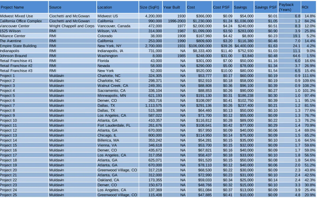
This Report looked at evidence from over 75 case studies. Using data from these case studies provides anecdotal evidence suggesting that AERs result in a wide range of returns in the commercial real estate market. Returns vary based on the size of the initial investment, larger investments necessary for deep retrofits having in general lower ROIs than the light ones (windows, insulation, light bulbs). In addition, the payback will also vary by building structure and age and whether there are energy inefficiencies to begin with; where there areare energy inefficiencies to begin with, there will be higher rate of returns. The payback will vary by region as pointed out in Jaffe et al. (2012), based on differing structure of energy pricing and energy sources. In Figure 2, we summarize 38 case studies that report information on costs of the AERs, energy savings, operational savings, and information on the financing of the investment. In particular, we focus on cases with sufficient information to quantify a payback period or simple one year Return on Investment (ROI). The retrofits reported in these case studies vary in how deep they are. Those in Muldavin (2009) are lighter while those reported in Ciochetti and McGowan (2010), by the Rocky Mountain Institute and by Wright Chappell and Corps (2010) are more extensive retrofits.
The first set of cases, reported in Muldavin (2009) constitutes of 25 retrofits on buildings that obtained the LEED-EB certification. These retrofits were undertaken on relatively large buildings (on average over 400, 000 square feet). On average these retrofits cost $86,455 ($0.21/SF) and saved $62,820 ($0.16/SF) annually with an average estimated payback of 1.38 years (ranging from 0.9 to 4.8 years). The one year ROI for these retrofits is on average of 67.7%. These are light retrofits with evidence of cost savings associated with reduction in energy consumption of 7.1% on average based on average energy cost for commercial buildings in the US of $2.21/SF (Econsult, 2010).
The second group of cases comprises three sets of studies: 2 projects analyzed by Ciochetti and McGowan (2010); 9 cases from the Rocky Mountain Institute; and one from Wright Chappell and Corps (2010). These 12 AERs have enough quantitative
13
information to allow for financial analysis. The retrofits reported were performed on large buildings or building portfolios (over 800,000 SF on average). From this set,
reported retrofits cost $10.1M ($10.03/SF) on average and provided savings of $591,913 (0.86/SF) on average annually with an average estimated payback of 13.52 years
(ranging from 1.4 to 64.6). The one year ROI for these retrofits is on average of 17.6%. These are deeper retrofits with evidence of cost savings associated with reduction in energy consumption of 39% on average.
These two groups of case studies represent very different depths of intervention and different types of buildings. These differences point how difficult it is to of standardize case studies and offer precise estimates of the costs and savings associated with AERs. Even when standardizing the costs per square foot, the investments vary by five orders of magnitude. The return on investments associated with AERs will vary significantly across building type, energy use intensity, geographic region, and whether the retrofit is "deep" or "low hanging fruit." More standardized studies are required to provide
comparative estimates of the costs associated with different levels of retrofits in different type of buildings. Such estimates are important both for owners to decide to invest the energy to engage an AER in their property and for lenders to underwrite the loans associated with such investments.
4. The Philadelphia Case
To identify the macro scale implications of energy efficient investments, this Report applies the findings of the previous sections to estimates of potential size of the market for energy retrofits in the Philadelphia region. In a report produced for the EEB Hub, Econsult Corporation (2011) analyzed commercial and industrial buildings in the Philadelphia area to determine the market for energy retrofits and estimated that this set of buildings included 9,058 commercial properties in the Greater Philadelphia region representing 397.5 million square feet (SF). Of those, 4,201 buildings (representing 154 million SF) could benefit from an AER.
The average annual energy cost for US commercial properties is $2.21 per square foot. In Philadelphia, this average is higher, and the typical commercial property spends $2.83 per year on energy costs (BOMA Experience Exchange Report for Philadelphia Area, 2011)—this is despite Econsult’s estimate that 18% of the commercial space in the Philadelphia region is eco-labeled. This result could be due to: a lower relative
concentration of eco-labels in Philadelphia versus nationally; a higher concentration of “energy hogs” among the non-labeled buildings; a higher relative cost of energy in Philadelphia; and/or eco-labeling that does not always correlate with levels of energy efficiency. Regardless of the cause, AERs could reduce the amount of energy spend for retrofitted building owners; moreover, in addition to energy savings, Econsult estimates that retrofitting the buildings identified as prime for AERs would generate $618m in local spending, and support 23,500 jobs. Based on this analysis this Report estimates the corresponding size of the green retrofit market in Philadelphia that would support this job creation. This requires an understanding of the mechanisms through which a building’s energy efficiency impacts its potential value.
14
Table 2: Findings from Case Studies—Cost and Savings Associated with EERs
Project Name Source Location Size (SqFt) Year Built Cost Cost PSF Savings Savings PSF Payback (Years) ROI Midwest Mixed Use Ciochetti and McGowan Midwest US 4,200,000 1930 $366,000 $0.09 $54,000 $0.01 6.8 14.8% California Office Complex Ciochetti and McGowan California 990,000 1996-2003 $1,230,000 $1.24 $1,036,000 $1.05 1.2 84.2% Vancouver Center Wright Chappell and Corps Vancouver, Canada 472,000 1977 $2,000,000 $4.24 $240,000 $0.51 8.3 12.0% 1525 Wilson RMI Wilson, VA 314,000 1987 $1,099,000 $3.50 $283,000 $0.90 3.9 25.8% Alliance Center RMI Colorado 38,000 1908 $167,960 $4.42 $8,800 $0.23 19.1 5.2% The Aventine RMI California 253,000 1990 $809,600 $3.20 $116,380 $0.46 7.0 14.4% Empire State Building RMI New York, NY 2,700,000 1931 $106,000,000 $39.26 $4,400,000 $1.63 24.1 4.2% Indianapolis RMI Indianapolis, IA 731,000 NA $8,333,400 $11.40 $752,930 $1.03 11.1 9.0% Johnson Braund RMI Washington 8,000 1985 $248,000 $31.00 $3,840 $0.48 64.6 1.5% Retail Franchise #1 RMI Florida 43,000 NA $301,000 $7.00 $50,000 $1.16 6.0 16.6% Retail Franchise #2 RMI Nevada 58,000 NA $290,000 $5.00 $78,000 $1.34 3.7 26.9% Retail Franchise #3 RMI New York 52,000 NA $520,000 $10.00 $80,000 $1.54 6.5 15.4% Project 1 Muldavin Charlotte, NC 324,305 NA $53,777 $0.17 $60,000 $0.19 0.9 111.6% Project 2 Muldavin Charlotte, NC 298,371 NA $52,910 $0.18 $58,000 $0.19 0.9 109.6% Project 3 Muldavin Walnut Creek, CA 249,391 NA $88,808 $0.36 $96,100 $0.39 0.9 108.2% Project 4 Muldavin Sacramento, CA 336,104 NA $88,853 $0.26 $90,000 $0.27 1.0 101.3% Project 5 Muldavin Minneapolis, MN 621,193 NA $191,130 $0.31 $186,238 $0.30 1.0 97.4% Project 6 Muldavin Denver, CO 263,716 NA $108,097 $0.41 $102,750 $0.39 1.1 95.1% Project 7 Muldavin Dallas, TX 1,113,575 NA $291,136 $0.26 $237,400 $0.21 1.2 81.5% Project 8 Muldavin Dallas, TX 515,388 NA $64,460 $0.13 $50,000 $0.10 1.3 77.6% Project 9 Muldavin Los Angeles, CA 587,022 NA $71,700 $0.12 $55,000 $0.09 1.3 76.7% Project 10 Muldavin Atlanta, GA 410,357 NA $116,812 $0.28 $89,000 $0.22 1.3 76.2% Project 11 Muldavin Fort Lauderdale, FL 261,676 NA $108,641 $0.42 $77,000 $0.29 1.4 70.9% Project 12 Muldavin Atlanta, GA 670,000 NA $57,950 $0.09 $40,000 $0.06 1.4 69.0% Project 13 Muldavin Chicago, IL 800,000 NA $114,950 $0.14 $75,000 $0.09 1.5 65.2% Project 14 Muldavin Billerica, MA 353,242 NA $54,281 $0.15 $35,000 $0.10 1.6 64.5% Project 15 Muldavin Vienna, VA 346,618 NA $53,700 $0.15 $32,000 $0.09 1.7 59.6% Project 16 Muldavin Denver, CO 435,672 NA $67,821 $0.16 $40,000 $0.09 1.7 59.0% Project 17 Muldavin Los Angeles, CA 317,058 NA $58,437 $0.18 $33,000 $0.10 1.8 56.5% Project 18 Muldavin Atlanta, GA 625,071 NA $91,520 $0.15 $50,000 $0.08 1.8 54.6% Project 19 Muldavin Atlanta, GA 670,000 NA $78,110 $0.12 $40,000 $0.06 2.0 51.2% Project 20 Muldavin Greenwood Village, CO 317,218 NA $68,530 $0.22 $30,000 $0.09 2.3 43.8% Project 21 Muldavin Atlanta, GA 312,000 NA $72,990 $0.23 $31,000 $0.10 2.4 42.5% Project 22 Muldavin Oakland, CA 173,355 NA $59,033 $0.34 $25,000 $0.14 2.4 42.3% Project 23 Muldavin Denver, CO 150,673 NA $48,766 $0.32 $15,000 $0.10 3.3 30.8% Project 24 Muldavin Los Angeles, CA 137,369 NA $51,084 $0.37 $13,000 $0.09 3.9 25.4% Project 25 Muldavin Greenwood Village, CO 115,408 NA $47,885 $0.41 $10,000 $0.09 4.8 20.9%
15
As discussed in further detail below, the basis of a single property’s value is its Net Operating Income (NOI), calculated as the gross revenues of the building (rents, expense reimbursements, ancillary income) less the operating expenses of the building (including maintenance, taxes, insurance, utilities and other energy costs). Once the NOI is
determined, the most common means of estimating the value of the building is to divide the NOI by a Capitalization (or “Cap”) Rate. The Cap Rate most simply is described as a measure of the relative worth of the building’s cash flows, or NOI, and takes into account such factors as location, relative risk of cash flows, quality of the asset (class A, B, etc.), competition of similar properties and other factors influencing demand for the asset. These two key metrics—NOI and Cap Rate—form the fundamentals of value. An owner can increase the value of the property by improving the NOI (reducing the operating costs or increasing the revenues) and/or by improving the Cap Rate. AERs can do both. AERs improve NOI by both reducing energy costs (which represent 25% of the operating expenses) and also can increase rents by reducing vacancy (Frew and Jud, 1998; Kok et al. 2012), and by increasing a tenant’s willingness to pay higher rents due to a higher worker productivity and a desire for “green” space and the reputational advantages associated with it (Chau et al., 2010). AERs can also decrease the Cap Rate—which improves the property’s value—since Cap Rates represent in-place yield of the asset, a higher Cap Rate is indicative of a higher risk investment, which lowers the underlying value. AERs can decrease the risk associated with a given cash flow (NOI), therefore decreasing the Cap Rate and increasing the property’s value. The decrease in risk provided by AERs includes: reducing the volatility of cash flow by limiting exposure due to: fluctuating energy prices, regulatory uncertainty, and the chance of obsolescence (see discussion of Jaffee et al. 2012 and Mills, 2003).
The literature on green labels for real estate provides insights into how energy efficiency contributes to the value of commercial properties. In particular, the hedonic studies of green label premia discussed above indicate that under current market conditions, green office space enjoys a considerable premium, outside of energy savings, and that energy efficiency contributes to value through both of these two ways: improving NOI (savings on energy, increases in rents) and from improving the Cap Rate through the reductions in risk/reward mentioned immediately above as well as through a
supply/demand dynamic that generates a green premium derived from increased demand for “green” real estate.
We can use data on average energy expenditures to illustrate the difference between the NOI effect and the Cap Rate effect in Energy Star buildings. Below, we use this data to demonstrate the NOI effect on value (figure 3) and the Cap Rate effect (figure 4). Following that we can size the total market for AERs in the Philadelphia case.
The Building Owners and Managers Association provides data on commercial real estate expenditures and income based on annual surveys. Figure 3 uses Building Owners and Managers Association (BOMA) data on NOI and operating expenses in the Philadelphia
16
market and Real Capital Analytics data reporting office cap rate of 7.1% in Philadelphia for 2012 to model the impact of energy efficiency derived NOI improvements associated with Energy Star.19 Energy efficiency per square foot values have been extrapolated for 20,000 SF, 50,000 SF, and 200,000 SF building cases to illustrate how the size of a building influences energy efficiency valuation improvements. Fields labeled “max investment” describe the added value associated with the retrofit; this also can be understood as the maximum amount an investor can spend on energy efficiency relative to the base case without incurring losses.
Table 3: Energy Efficiency and Value Premia Due to Cost Savings in Commercial Real Estate—the Philadelphia Case
Average Building 20% Efficiency Improvement
Average Total Operating Expenses per ft2 $10.15 $9.72
Total Income per ft2 $25.52 $25.52
NOI per ft2 $15.37 $15.80
Cap Rate 7.1% 7.1%
Annual Savings per ft2 - $0.44
Value per ft2 $216.48 $222.54
Value premium - 2.8%
Value added per ft2 Investment - $6.06
Value of a 20k ft2 Building $4,329,577 $4,450,704
Value of a 50K ft2 Building $10,823,943 $11,126,760
Value of a 200k ft2 Building $43,295,774 $44,507,042
Max Investment for 20k ft2 Building - $121,126
Max Investment for 50k ft2 Building - $302,816
Max Investment for 200k ft2 Building - $1,211,267
In contrast to energy efficiency NOI improvements through energy savings, and similar to improved Willingness-to-Pay NOI effects, Cap Rate effects are difficult to isolate. As discussed above, Cap Rate effects result from increased demand for green space and from improvements in the risk/reward investment equation by offsetting risks of
fluctuating energy prices, regulatory uncertainty, and the chance of obsolescence. These effects are not easily factored into valuation, however, the literature suggests that there are real premiums derived from consumer preference for green buildings and supports an association between green label buildings and lower cap rates. Both Fuerst and McAllister (2011) and Pivo and Fisher (2010) found that cap rates were approximately 50 basis points, or 0.5 %, lower in green label buildings than conventional buildings. Figure 4 shows the impact a 0.5% lower cap rate has on value when combined with energy efficiency derived premiums described in Figure 3.
19
Note that we are only demonstrating here the improved NOI from cost savings—as noted above, there are also further potential improvements in NOI from increased willingness-to-pay and decreased vacancy
17
Table 4: Energy Efficiency and Value Premia Due to Cap Rate Effects in Commercial Real Estate—the Philadelphia Case
Building Average Improvement 20% Efficiency
Average Total Operating Expenses per
ft2 $10.15 $9.72
Total Income per ft2 $25.52 $25.52
NOI per ft2 $15.37 $15.80
Cap Rate 7.1% 0.066
Annual Savings per ft2 - $0.44
Value per ft2 $216.48 $239.39
Value premium - 10.6%
Max per ft2 Investment - $22.92
Value of a 20k ft2 Building $4,329,577 $4,787,879
Value of a 50K ft2 Building $10,823,944 $11,969,697
Value of a 200k ft2 Building $43,295,775 $47,878,788
Max Investment for 20k ft2 Building - $458,301
Max Investment for 50k ft2 Building - $1,145,753
Max Investment for 200k ft2 Building - $4,583,013
Figure 4 shows that the literature suggested Cap Rate improvement causes significantly higher premia than that experienced due to NOI improvements alone. Combining the NOI Effects (figure 3) and Cap rate effects (figure 4) makes a strong financial case for investing in green buildings for small (as well as large) building owners. Given the observations made for the “average” building as discussed in the two figures above, we estimate the size of a potential market for AERs in the Philadelphia case. We know that on average, Philadelphia commercial buildings spend $2.83 per SF per year on energy consumption (BOMA Experience Exchange Report for Philadelphia Area, 2011). Based on the EEB Hub’s energy consumption reduction goal we model the impact of a 20% efficiency improvement. From Econsult’s study we estimate 154 million SF of
commercial office in the Philadelphia case is a good target for AERs. We then calculate the annual NOI improvements associated with a 20% energy saving as follows:
($2.83 / SF) * (20% Savings) * (154 M SF of target space) = $87.2 million This number represents the NOI improvements due to cost savings alone. Therefore these would be in our estimation conservative numbers for direct value improvements. In order to turn annual NOI savings into valuation impacts, we must use the value equation:
18
Using a Philadelphia office market Cap Rate of 7.1% (as calculated by Real Capital Analytics for 2012), we can size the market for AERs:
Value, Estimate for 20% Savings = (87.2 million) / (7.1%) = $1.2 Billion
This number represents the forecasted increased asset value in aggregate across the Philadelphia commercial office market. These numbers do not include increasing NOI through improved willingness to pay. Therefore, the actual market may be larger.
5. Economics of Energy Efficient Retrofits
The core market concept of single property real estate economics is the value equation: how the valuation of a building asset relates to its existing cash flow, its competitive set and its relative risk as an investment. This market approach is focused heavily on the purchaser and seller as the prime agents, and therefore emphasizes arbitrage between
price and long term economic value:20 a good price is one which is lower than or equal to the long term discounted, risk-adjusted value (NPV Positive). Appraisers have a more generalized responsibility, to assess value today. The Appraisal Institute lists three ways of determining the assessed value of a building: sales comparables,
replacement/construction cost, and the income approach.21 These three are all valid ways for determining the value for a building.22
However, core investors and owners in the private commercial real estate market primarily rely on just one of these methods to determine price: the income approach (ULI, 2009). The reason for this is that the income approach is the only one of the three that is built upon an investment framework of fundamental value: how what one pays for an asset relates to (i) the income that the asset can generate; and (ii) the risk-adjusted return of this asset versus its peers. Commonly, income is expressed as Net Operating Income (NOI) and anticipated risk-adjusted return in the form of a
capitalization rate (CR).23 The value equation can then be expressed as: BUILDING VALUE = NOI / CR
NOI is calculated as gross property income less vacancy and operating expenses— notably it does not include debt service payments, taxes or capital expense allocations. The CR is a ratio used to estimate the value of the revenue stream (for income
producing properties), and contributes to the value equation an accounting for risk, real
20 Public policy can be used to re-align price with social good, such as reduced energy consumption. In this paper, however, we are concerned with endemic economics of EER.
21
The Appraisal of Real Estate, p. 582 (AIREA, 9th Ed., 1987)
22 Commercial real estate investors can propose a thesis for uncovering properties where there is inefficient pricing: that is, when price and value do not match. This is exactly the type of strategy available during the EE adoption curve.
23
Anticipated risk adjusted return (CR in the value equation) is not to be confused with current in-place yield. The CR is a predictive value, estimating the long term expectation of the value of currently in-place cash flows.
19
estate cycle, location and other ( capitalized) considerations.24 In looking at the value equation, we can see simply that a building’s value goes up as: (a) the NOI increases (operational changes); or (b) the CR decreases (market pricing changes).
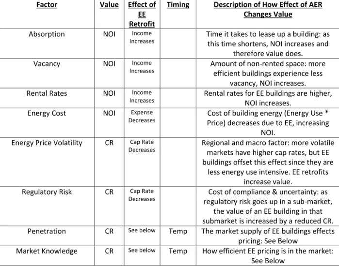
As such, we can divide AERs into two categories: impacting NOI or CR. Table 5: NOI and CR Effects of AERs
Factor Value Effect of
EE Retrofit
Timing Description of How Effect of AER
Changes Value
Absorption NOI Income
Increases Time it takes to lease up a building: as this time shortens, NOI increases and
therefore value does.
Vacancy NOI Income
Increases Amount of non-rented space: more efficient buildings experience less
vacancy, NOI increases.
Rental Rates NOI Income
Increases Rental rates for EE buildings are higher, NOI increases.
Energy Cost NOI Expense
Decreases Price) decreases due to EE, increasing Cost of building energy (Energy Use *
NOI.
Energy Price Volatility CR Cap Rate
Decreases Regional and macro factor: more volatile markets have higher cap rates, but EE
buildings offset this effect since they are less energy use intensive. EE retrofits
increase value.
Regulatory Risk CR Cap Rate
Decreases regulatory risk goes up in a sub-market, Cost of compliance & uncertainty: as
the value of an EE building in that submarket is increased by a reduced CR.
Penetration CR See below Temp The market supply of EE buildings effects
pricing: See Below
Market Knowledge CR See below Temp How efficient EE pricing is in the market:
See Below
The factors that affect NOI are all measurable, although in some cases attributing them to an AER can be difficult. As discussed above, in the literature, there are numerous studies that establish a correlation between green labels and valuation. To review here: Miller et al. (2008) perform a hedonic regression controlling for age, proximity to CBD, and metropolitan area and report value premiums of approximately 6% for Energy Star, and 10% for LEED.25 Wiley et al. (2010) use CoStar 2008 data on class A office space—a
24 This is a vastly simplified explanation of cap rates. For a more detailed analysis see: Geltner, David; Miller, Norman G., Clayton, Jim; Eichholtz, Piet; Commercial Real Estate Analysis and Investments. 2nd Ed. Dec. 2006.
20
total of 7,300 properties for rental and 1,151 for sales price—estimating rent premiums at 7.3% (Energy Star) and 15.2% (LEED), and sales premiums at $29-$129/SF.26 Fuerst and McAllister’s (2011) sales price regression indicate much larger effects with 30% premiums associated with green labels, 25% premiums with LEED, 26%-27% with Energy Star. Eichholtz et al. (2010) find that a combined green label is associated with a 3.5% rent premium and a statistically significant premium associated with LEED, but did find a highly significant premium for Energy Star of 3.3%.
These results vary widely because: (a) green labels are serving as a proxy for quantifiable economic factors; (b) markets are in the midst of an adoption curve; and (c) the studies sometimes are measuring different things due to variance in the underlying data sets utilized.27 Assuming even a constant income stream AERs increase NOI by lowering operating costs. 28
This Report reviews 75 case studies of AERs. First, a set of 25 retrofits reported in Muldavin (2009) costing an average of $86,455 ($0.21/SF) with an average estimated payback of 1.38 years (and an average first year savings of $62,820). The second group of case studies was assembled from work done by the Rocky Mountain Institute,29 Wright Chappell and Corps (2009), and Ciochetti and McGowan (2010): we selected all of the cases that had enough quantitative information to allow for simple analysis, revealing 12 retrofits costing an average of $10.1M ($10.03/SF) with an average estimated payback of 13.52 years (and an average annual savings of $591,913). These two sets represent outcomes of different depths of intervention. Nonetheless large positive impacts on NOI are shown and again overall market conditions will matter.
Cap Rates: Market Information, Regulatory Risk, and the Brown Discount Since the AER market is still in its early development phases, it is subject to an adoption curve that causes market effects. There are three main causes of these effects: level of sub-market penetration, market knowledge asymmetry and regulatory risk. On the adoption curve, Andrew Nelson of RREEF notes:
‘‘...many major markets will reach the critical mass where green buildings account for enough of the building stock that tenants have a choice. At this point, the performance premiums for green buildings will flip to a discount for older, less efficient, conventional buildings. We are already at or near this point in the mature
26 Information not provided to translate sales premiums to percentage values.
27 Energy cost reduction is the source, along with tenant productivity, of the payback results for AERs. The former is fully quantifiable with a growing number of case studies and examples, as discussed above. This presupposes a solution to Jevon’s Paradox: that as a building becomes more energy efficient, the user of the building uses more energy, since it is cheaper. This is a substantive issue, but is more accurately described as an agency problem than a paradox. Solutions to this paradox abound in both the public side (regulation, disclosure) and the private side (incentive leases, energy price).
28
That is, ignoring the other potential positive effects of absorption, vacancy, rent increases. 29 Rocky Mountain institute, http://www.rmi.org/retrofit_depot_get_connected_true_retrofit_stories
21
economies of Europe and developed Asia, and getting closer in the major money centers of the United States,’’ (Nelson, 2009).30
Each of these market factors has a CR effect driven by three market specific factors: market penetration, regulatory risk, and market knowledge.
Figure 1: Market Penetration of AERs
To illustrate these CR effects, we use a hypothetical representation of the Philadelphia Office market. Our hypothetical example shows Philadelphia office pricing at two time periods, representing a low level of AER building penetration (Period 0, left) and a much higher level of AER penetration (Period 1, right).
Market Penetration: Each market has a different adoption rate—the rate at which AER buildings become the norm. A more specific effect observed in new markets is the substitution effect: when there are fewer AER buildings available, a buyer will increase the price they are willing to pay beyond what would be expected from NOI effects alone. This should be related to the new general state of market equilibrium. This is
30Runde and Thoyre (2010) apply this idea to appraisal characteristics. They focus on the NOI effects on
overall valuation: that is, how market rents will vary with market penetration. In general, they contend that the effect on valuation of a green (and for us AER) building will change with time, experiencing an inflection point at which premia to green turn into discount to brown. In addition to this noted NOI effect, there also is likely to be a CR effect.
22
basic supply/demand, and feeds the pipeline for new AER buildings (Runde and Thoyre, 2010).
In the example above, Period 0 shows AER buildings at approximately 20% of the market, and trading at a 50 bps spread CR over non AER (6.5% vs. 7.0%). In Period 1, as market penetration of AER passes the inflection point, the CR spread of AER over non-AER increases to 100 bps, as the higher risk associated with non-energy efficient buildings is recognized. 31 It is vital to note here that NOI effects due strictly to AER retrofits remain exactly the same at both levels of market penetration because these are tied to direct operating savings.
Market Knowledge: Since market knowledge lags behind market propagation, there can be information asymmetry in a new market composed only of local actors. In real
estate, information asymmetry most commonly leads to the “winner’s curse” in which the bid winning party is willing to pay more. In this case, a party (or counter-bidder) with less knowledge about AERs would be outbid by the buyer who uses information to arbitrage energy efficient investments that are not fully valued. Regulatory Risk: This factor points to the risk associated with uncertainty as to the future of regulation in a market. Currently, markets have very different regulatory frameworks with relation to energy and AERs. As both the cost of compliance and uncertainty increase in a market, the value of an AER building is increased by a reduced cap rate.
Cost of Capital and Risks and Volatility of Energy Costs
Besides the risks of investing in real estate, there is the cost of borrowing for these investments. Jaffee, Stanton and Wallace (2012) evaluate commercial office mortgage underwriting and find that standard practices for making loans on these properties do not take into account energy efficiency’s key contribution to potential default risk. Given that energy prices are highly volatile, and energy efficient buildings are less exposed to that volatility, EE buildings should have less default risk, be less expensive to finance per square foot and therefore more attractive to investors. However, the authors find that existing loan practices provide no incentive for doing AERs. Standard underwriting focuses on managing interest rate risk and market pricing dynamics, as well as evaluating potential pre-payment risk and overall default (credit) risk. The authors develop a theoretical model that extends standard underwriting to manage risks associated with energy: electrical/gas pricing dynamics and location dynamics of energy pricing. They then back-test this theoretic model to calibrate it against known valuation results and find that building loans can—and in their opinion should—be differentiated based on energy efficiency. This change in valuation due to decreased risk exposure of the cash flows would be captured in a lower cost of finance and cap rate.
31
In essence, empirical work can reveal a Period 0 to Period 1 CR compression as shown in the
hypothetical Philadelphia example above. For REITs, a similar strategy can be employed to immediately increase dividends.
23
To estimate how much of an impact this might have on the cost of finance, Jaffe et al. (2012) analyze the geography of energy risk in the US to demonstrate that energy pricing and volatility is affected by measurable and known factors: the nodal structure of natural gas delivery, the proximity to electricity pricing hubs and the geography of proximate population centers. Their conclusion is that there is no national market for electricity or gas, but that building location can serve as a proxy for relative energy risk and that a building’s level of energy efficiency can then indicate the level of exposure to that relative energy risk.
Since energy prices for electricity and gas vary across space and over time, so too must the NOI of the corresponding buildings, since energy costs represent approximately 12% of gross rent and 30% of costs (BOMA). By extending underwriting to take into account the exposure to energy price volatility, underwriters manage the risk linked to electrical and gas pricing dynamics and location dynamics. Jaffe et al. use these two factors: building location and building level of EE to develop a commercial-mortgage valuation model accounting for energy risks. In order to develop this model, the authors must measure both consumption of energy and volatility of energy pricing. Providing an accurate measure of consumption and volatility for underwriting purposes is costly and can prove difficult. There are five main methods of approach. The first is measuring utility bills—but these are not always available, and even when available cannot be easily related to building systems, relative occupancy and equipment. The second is using the DOE/EPA Energy Star and Portfolio Manager system—but lenders cannot directly correlate these systems to energy. For the next two methods: simulation and regression—the available data are insufficient and the buildings too heterogeneous to successfully execute. As a result of these limitations the authors favor the fifth method, benchmarking, to calculate the Energy Use Intensity (EUI) of a building compared to peer group and use its location to determine that volatility and pricing.
Jaffee et al. (2012) use two datasets for this benchmark: the Commercial Buildings Energy Consumption Survey (CBECS) that collects extended information about 5,215 buildings across country, and the California Commercial End-Use Survey that collects data about 2,790 commercial buildings with information about the utility area, the region’s climate, the building type and its EUI.32 Their results indicate that not explicitly accounting for energy volatility leads to mortgage mispricing. Their simulations show that the inclusion of energy risk reduces commercial mortgage mispricing by 8.5%.
Implications for the Cap Rate
While short term conditions in sub-markets persist (in the form of low market penetration and low market knowledge of AERs), investment opportunities exist. In single building investment, consider three buildings with identical NOI: (a) “brown building”; (b) an AER building; and (c) a green label building. In each case, the NOI will reflect the value of the cash flow, already capitalizing into the value equation the worth
32
Limitations associated with these datasets are that they do not have information about relative energy efficiency, that they exclude some of the important MSAs and that they do not differentiate the climates within large regions.
24
of any consumption savings (or the discount due to their lack). Since we are in a low penetration market, we can assume several things: there is a significant CR spread from brown to AER; there is room for NOI improvement with short-term AER payback; and there is low market knowledge of buyers and sellers as to the previous two
assumptions. As a buyer, then, the opportunistic strategy is to “Buy Brown, and Turn it Around” to take advantage of NOI effects as well as NOI volatility effects that, once recognized, will be positively impact buildings with AERs. As volatility effects are
capitalized, greater than warranted for the risk of the investment. in the long run, a cap rate differential remains, both due to lower NOI volatility and exposure to regulatory risk.
25
Conclusion
This Report provides information on the identification of the value premiums (price, rent) associated with energy efficient buildings in the commercial office sector. Recent studies that use hedonic regression techniques (Kok et al., 2012; Pivo and Fisher, 2010; Eichholtz et al., 2010; Wiley et al., 2010; Fuerst and McAllister, 2011; and Miller et al., 2008), establish value premiums of 6% for rents and 15% for prices attributed to buildings with LEED and Energy Star labels. In addition, the Report assembles case studies to further analyze the underlying economics of AERs. One group of case studies includes light retrofits that on average: have energy saving of 7.1%, an estimated
payback of 1.4 years and yield a one year ROI of 67.7%. The other includes deep retrofits that on average: save 39% of energy consumption, pay back in 13.5 years and return 17.7% on invested capital. More studies are required to provide standardized estimates of the costs associated with different levels of retrofits in different type of buildings. Such estimates are important both for owners to decide to invest the energy to engage an AER in their property and for lenders to underwrite the loans associated with such investments. These case studies show the potential for financing retrofits purely based on cash flow improvements due to energy savings.
The Report combines these findings with Philadelphia specific information to highlight “The Philadelphia Case.” By forecasting the increase in asset value due to cost savings across an energy efficient retrofit of the Philadelphia commercial office market, the Report estimates the potential market activity to be over $1 Billion from AERs financed purely from energy savings that increase net cash flows (NOI).
AERs improve NOI not just by lowering energy costs but also by increasing a tenant’s willingness to pay higher rents for productivity improvements or reputational
advantages. Moreover, AERs also decrease the Cap Rate—which improves the
property’s value—by reducing the volatility of cash flows by limiting exposure due to: fluctuating energy prices, regulatory uncertainty, and the chance of obsolescence. This is a period of change for the energy efficiency building market, and some of these effects are short term—effects of limited market penetration (that reduces as more efficient buildings come on line) or information asymmetry (addressed by the increasing prevalence of energy disclosure laws). But some effects are permanent: the cost savings from reduced energy intensity, the decrease in exposure to energy price volatility and the defense against changing efficiency regulation.
In 2010, commercial buildings accounted for 19% of US energy consumption, making the sector an important target of the efforts to reduce environmental impact, achieve energy independence, and increase productivity through energy efficiency. In addition to the potential for net social benefits, energy efficiency reduces building operation expenses, creating a private interest for building owners to invest in energy efficiency. Energy efficient buildings account for an ever increasing share of the commercial office market and we can expect that increase to continue, even as non-efficient buildings experience a “brown discount.” Private investors can take advantage of this evolving
26
market to increase profitability. Increased standardized information provided by disclosure policies, building rating systems and data aggregation and analysis can be helpful in speeding the adoption of energy efficiency in the marketplace and improving the timetable for achieving reduced energy consumption even as they increase
27
Bibliography
Anderson, Soren T., and Richard G. Newell. Information Programs for Technology
Adoption: The Case of Energy-Efficiency Audits. Resource and Energy Economics, (2004). 26. 1: 27–50.
Chao, M., and Gretchen Parker. Recognition of energy costs and energy performance in commercial property valuation. New York, NY: New York State Energy Research and Development Authority, 2000.
Chau, C-K., M.S. Tse, and K.Y. Chung. A Choice Experiment to Estimate the Effect of Green Experience on Preferences and Willingness-to-Pay for Green Building Attributes. Building and Environment, (2010), 45.11: 2553–61.
Ciochetti, B. A. and M. D. McGowan. “Energy Efficiency Improvements: Do they Pay?”
Journal of Sustainable Real Estate, (2010), 2.1: 305-333.
Dermisi, Sofia and McDonald, John. “Effect of ‘Green’ (LEED and Energy Star)
Designation on Prices/SF and Transaction Frequency: the Case of the Chicago Office Market,” Journal of Real Estate Portfolio Management, (2011). 17.1.
Dermisi, S. “Effect of LEED Ratings and Levels on Office Property Assessed and Market Values.” Journal of Sustainable Real Estate, (2009). 1.1: 23–47.
Diamond, Rick. "Evaluating the energy performance of the first generation of LEED-certified commercial buildings." (2011). Available at
http://escholarship.org/uc/item/498009ks#page-2.
Dunse, Neil, and Colin Jones. "A hedonic price model of office rents." Journal of Property Valuation and Investment, (1998). 16.3: 297-312.
Econsult Corporation. “The Market for Commercial Property Energy Retrofits in the Philadelphia Region.” October 2011.
http://www.eebhub.org/media/files/eebhub_reports_energy-market.pdf.
Energy Information Administration. “Commercial Buildings Energy Consumption Survey: Building Characteristics Tables; Table B9. Washington DC. (2006).
Eichholtz, Piet, Nils Kok, and John M. Quigley. "Doing Well by Doing Good: Green Office Buildings." American Economic Review, (2010). 100.5: 2494–511.