Intended for submission to the28th Annual ACM SIGPLAN-SIGACT Symposium on Principles of Programming Languages
An Abstract Monte-Carlo Method for the Analysis of
Probabilistic Programs
∗
David Monniaux
´
Ecole Normale Sup´erieure
Laboratoire d’Informatique 45, rue d’Ulm 75230 Paris cedex 5 France[email protected]
ABSTRACT
We introduce a new method, combination of random test-ing and abstract interpretation, for the analysis of programs featuring both probabilistic and non-probabilistic nondeter-minism. After introducing “ordinary” testing, we show how to combine testing and abstract interpretation and give for-mulas linking the precision of the results to the number of iterations. We then discuss complexity and optimization is-sues and end with some experimental results.
1
INTRODUCTION
We introduce a generic method that lifts an ordinary ab-stract interpretation scheme to an analyzer yielding upper bounds on the probability of certain outcomes, taking into account both randomness and ordinary nondeterminism.
1.1
Motivations
It is sometimes desirable to estimate the probability of cer-tain outcomes of a randomized computation process, such as a randomized algorithm or an embedded systems whose environment (users, mechanical and electrical parts. . . ) is modelized by known random distributions. In this latter case, it is particularly important to obtain upper bounds on the probability of failure.
Let us take an example. A copy machine has a comput-erized control system that interacts with the user through ∗This work was partially funded by Commissariat `a l’´Energie Atomique under contract 27234/VSF.
c
-Notice
some control panel, drives (servo)motors and receives infor-mation from sensors. In some circumstances, the sensors can give bad information; for instance, some loose scrap of paper might prevent some optical sensor from working cor-rectly. It is nevertheless desired that the probability that the machine will stop in an undesired state (without having returned the original, for instance) is very low given some re-alistic rates of failure from the sensors. To make the system more reliable, some sensors are redundant and the control-ling algorithm tries to act coherently. Since adding sensors to the design costs space and hardware, it is interesting to evaluate the probabilities of failure even before building a prototype. A similar case can be made of industrial systems such as nuclear power plants were sensors have a limited life time and cannot be expected to be reliable. Sound analysis methods are especially needed for that kind of systems as safety guidelines are often formulated in terms of maximal probabilities of failures [8].
Treating the above problem in an entirely probabilistic fashion is not entirely satisfactory. While it is possible to modelize the user by properties such as “the probability that the user will hit the C key during the transfer of double-sided documents is less than 1%”, this can prevent detecting some failures. For instance, if pressing some “unlikely” key combi-nation during a certain phase of copying has a good chance of preventing correct accounting of the number of copies made, certain users might use it to get free copies. This is certainly a bug in the system. To account for the behavior of inputs that cannot be reliably modelized by random distributions (for instance, malicious attacks) we must incorporate non-determinism.
1.2
Comparison to other works
An important literature has been published on software test-ing [11, 15, . . . ]; the purpose of testing techniques is to discover bugs and even to assert some sort of reliability cri-terion by testing the program on a certain number of cases. Such cases are either chosen randomly(random testing) or according to some ad hoc criteria, such as program state-ment or branch coverage(partition testing). Partition-based methods can be enhanced by sampling randomly inside the partition elements. Often, since the actual distribution in production use is unknown, an uniform distribution is as-sumed.
In our case, all the results our method gives are relative to some fixed, known, distributions driving some inputs. On the other hand, we will not have to assume some known distribution on the other inputs: they will be treated as nondeterministic. We thus avoid all problems pertaining to arbitrary choices of partitions or random distributions; our method, contrary to most testing methods, is fully mathe-matically sound.
There exists a domain called probabilistic software engi-neering[12] also aiming at estimating the safety of software. It is based on statistical studies on syntactic aspects of source code, or software engineering practices (programming lan-guage used, organization of the development teams . . . ), trying to estimate number of bugs in software according to recorded engineering experience. Our method does not use such considerations and bases itself on the actual software only.
Our analysis is based on a semantics equivalent to those proposed by Kozen [6, 7, 2nd semantics] and Monniaux [9]. We proposed a definition of abstract interpretation on prob-abilistic programs, using sets of measures, and gave a generic construction for abstract domains for the construction of an-alyzers. Nevertheless, this construction is rather “algebraic” and, contrary to the one explained here, does not make use of the well-studied properties of probabilities.
Several schemes of guarded logic commands [3] or refine-ment [10] have been introduced. While these systems are based on semantics broadly equivalent to ours, they are not analysis systems: they require considerable human input and are rather formal systems in which to construct derivations of properties of programs.
1.3
Contribution
We introduce for the first time a method combining statisti-cal and static analyses. This method is proven to be math-ematically sound. While some other methods have been re-cently proposed to statically derive properties of probabilis-tic programs in a general purpose programming language [9], ours is to our knowledge the first that makes use of statistical convergences.
1.4
Structure of the paper
We shall begin by an explanation of ordinary testing and its mathematical justification, then explain our “abstract Monte-Carlo” method. We shall then give the precise con-crete semantics that an abstract interpreter must use to im-plement our method. We shall finish with some early results from our implementation.
We shall take as an example a simple imperative language. Our method is by no means limited to imperative program-ming, but we found this choice to be both close to the most common programming uses and relatively simple to explain our method on.
2
ABSTRACT MONTE-CARLO: THE
IDEA
In this section, we shall explain, in a mathematical fashion, how our method works.
2.1
The Ordinary Monte-Carlo Testing
Method
Let us consider a deterministic programcwhose inputxlies inX and whose output lies inZ. We shall note [[c]] :X 7→Z
the semantics ofc(so that [[c]](x) is the result of the compu-tation ofcon the inputx). We shall takeX andZtwo mea-surable spaces and constrain [[c]] to be measurable. These measurability conditions are technical and do not actually restrict the scope of programs to consider [9]. For the sake of simplicity, we shall suppose in this sub-section thatc al-ways terminates.
Let us considerW ⊆Z a measurable set of final states whose probability we wish to measure whenxis a random variable whose probability measure isµ. The probability of
W is thereforeµ([[c]]−1(W)). Noting
tW(x) = 1 if [[c]](x)∈W
0 otherwise,
this probability is the expectation EtW. The law of large
numbers says that if we independently choose inputs xk,
with distributionµ, and compute the experimental average ¯ t(Wn) = n1 n k=1tW(xk), then limn→∞¯t (n) W =EtW. We can
even evaluate the probability of underestimating the prob-ability by more thantusing the Chernoff-Hoeffding [4] [14, inequality A.4.4] bounds:
Pr X¯
(n)
−EX≥t ≤e −2nt2
(1) TakingX= 1−tW, it follows that
Pr EtW ≥¯t
(n)
W +t ≤e −2nt2
(2) This method suffers from two drawbacks that make it un-suitable in certain cases:
• It supposes that all inputs to the program are either constant or driven according to a known probability distribution. In general, this is not the case: some in-puts might well be only specified by intervals of possible values, without any probability measure. In such cases, it is common [11] to assume some kind of distribution on the inputs, such as an uniform one for numeric in-puts. This might work in some cases, but grossly fail in others, since this is mathematically unsound.
• It supposes that the program terminates every time within an acceptable delay.
We propose a method that overcomes both of these prob-lems.
2.2
Abstract Monte-Carlo
We shall now consider the case where the inputs of the pro-gram are divided in two: those, inX, that follow a random distributionµand those that simply lie in some setY. Now [[c]] : X×Y → Z. The probability we are now trying to quantify isµ{x∈X | ∃y∈Y [[c]]hx, yi ∈W}. Some techni-cal conditions must be met so that this probability is well-defined; namely, the spacesXandY must be standard Borel
spaces [5, Def. 12.5].1 Since countable sets, , products of sequences of standard Borel spaces are standard Borel [5,
§12.B], this restriction does not concern most semantics. Noting
tW(x) = 1 if∃y∈Y [[c]]hx, yi ∈W
0 otherwise, this probability is the expectationEtW.
While it would be tempting, we cannot use a straight-forward Monte-Carlo method since, in general, tW is not
computable.2
Let us first recall the mathematical foundations of ab-stract interpretation [2, 1]. Let us now consider two pre-ordered setsA] and Z] so that there exist monotone func-tions γA :A] → (A), where A=X×Y, and γW :Z
] →
(Z), where (Z) is the set of parts of set Z, ordered by inclusion. The elements inA] andZ] represent some
prop-erties; for instance, ifX=
mandY =
n,A]could be the
set of descriptions of polyhedra in
m+nandγ
Athe function
mapping the description to the set of points inside the poly-hedron [2]. We then define anabstract interpretationof programcto be a monotone function [[c]]]:A]→Z]so that
∀a]∈A], ∀a∈A a∈γA(A])⇒[[c]](a)∈γB◦[[c]]](a]).
Let us also suppose that we can compute the following functions:
• I:X →A] so that
∀x∈X γA◦I(x)⊇ {x} ×Y;
• τW :Z] → {0,1}so that for allz]∈Z],τW(z]) = 0⇒
γZ(z])∩W =∅.
It is then possible to compute a functionTW suitable for our
needs: TW =τW ◦[[c]]]◦I.
We shall see in the following section how to build abstract interpreters with a view to using them for this Monte-Carlo method.
1Let us supposeX and Y are standard Borel spaces [5,
§12.B]. X×Y is thus a Polish space [5, §3.A] so that the first projection π1 is continuous. Let A ={x ∈ X | ∃y ∈
Y [[c]]hx, yi ∈ W}; then A =π1([[c]]−1(W)). Since [[c]] is a measurable function and W is a measurable set, [[c]]−1(W) is a Borel subset in the Polish spaceX×Y. Ais therefore analytic [5, Def. 14.1]; from Lusin’s theorem [5, Th. 21.10], it is universally measurable. In particular, it isµ-measurable [5,§17.A]. µ(A) is thus well-defined.
2Let us take a Turing machine (or program in a Turing-complete language)F. There exists an algorithmic transla-tion takingF as input and outputting the Turing machine
˜
F computing the total functionϕF˜ so that
ϕF˜hx, yi= 1 ifF terminates inyor less steps on inputx 0 otherwise.
Let us takeX = Y = andZ ={0,1} and the program ˜
F, and define t{1} as before. t{1}(x) = 1 if and only if F terminates on inputx. It is a classical fact of computability theory that thet{1}function is not computable for allF[13].
3
A CONCRETE SEMANTICS
SUIT-ABLE FOR ANALYSIS
From the previous section, it would seem that it is easy to use any abstract interpreter in a Monte-Carlo method. Alas, we shall now see that special precautions must be taken in the presence of calls to random generators inside loops.
3.1
Concrete Semantics
We have for now spoken of deterministic programs taking one inputx chosen according to some random distribution and one inputyin some domain. Calls to random generators (such as the POSIXdrand48() function) are usually mod-elized by a sequence of independent random variables. If a bounded number of calls (≤N) to such generators is used in the program, we can consider them as input values: xis then a tuplehx1, . . . , xN, viwherex1,. . .,xnare the values
for the generator andv is the input of the program. If an unbounded number of calls can be made, it is tempting to consider as an input a countable sequence of values (xn)n∈ where x1 is the result of the first call to the generator, x2 the result of the second call. . .; a formal description of such a semantics has been made by Kozen [6, 7].
Such a semantics is not very suitable for program analysis. Intuitively, analyzing such a semantics implies tracking the number of calls made to number generators. The problem is that such simple constructs as:
if (...) { random(); } else {}
are difficult to handle: the countings are not synchronized in both branches.
We shall now propose another semantics, identifying oc-currences of random generators by their program location and loop indices. The Backus-Naur form of the program-ming language we shall consider is:
instruction ::=elementary | instruction ;instruction | ifboolean expr theninstruction elseinstruction endif
| whileboolean expr
doinstruction
done
We leave the subcomponents largely unspecified, as they are not relevant to our method. elementary instructions are deterministic, terminating basic program blocks like as-signments and simple expression evaluations. boolean expr boolean expressions, such as comparisons, have semantics as sets of acceptable environments. For instance, aboolean expr expression can bex < y + 4; its semantics is the set of exe-cution environments where variablesxandyverify the above comparison. If we restrict ourselves to a finite numbernof integer variables, an environment is just an-tuple of integers. The denotational semantics of a code fragmentcis a map-ping from the setX of possible execution environments be-fore the instruction into the setY of possible environments after the instruction. Let us take an example. If we take
environments as elements of
3, representing the values of three integer variables x, y and z, then [[x:=y+z]] is the strict function hx, y, zi 7→ hy+z, y, zi. Semantics of basic constructs (assignments, arithmetic operators) can be easily dealt with this forward semantics; we shall now see how to deal with flow control.
The semantics of a sequence is expressed by simple com-position
[[e1; e2]] = [[e2]]◦[[e1]] (3) Tests get expressed easily, using as the semantics [[c]] of a boolean expressioncthe set of environments it matches:
[[if c then e1 else e2]](x) =
ifx∈[[c]] then [[e1]](x) else [[e2]](x) (4) and loops get the usual least-fixpoint semantics (considering the point-wise extension of the Scott flat ordering on partial functions)
[[while c do f]] = lfp(λφ.λx.
ifx∈[[c]] thenφ◦[[f]](x) elsex). (5) Non-termination shall be noted by⊥.
As for expressions, the only constructs whose semantics we shall precise are the random generators. We shall con-sider a finite setGof different generators. Each generatorg
outputs a random variablerg with distributionµg; each call
is independent from the precedent calls. Let us also con-sider the set P of program points and the set
∗ of finite sequences of positive integers. The set C = P×
∗ shall denote the possible times in an execution where a call to a random generator is made:hp, n1n2...nlinotes the execution
of program pointpat then1-th execution of the outermost program loop,. . .,nl-th execution of the innermost loop at
that point. Cis countable. We shall suppose that inside the inputs of the program there is for each generatorg inGa family (ˆghp,wi)hp,wi∈C of random choices.
The semantics of the language then become:
[[e1; e2]] = [[e2]]◦[[e1]] (6) Tests get expressed easily, using as the semantics [[c]] of a boolean expressioncthe set of environments it matches:
[[if c then e1 else e2]].hw, xi=
ifx∈[[c]] then [[e1]].hw, xielse [[e2]].hw, xi (7) Loops get the usual least-fixpoint semantics (considering the point-wise extension of the Scott flat ordering on partial functions):
[[while c do f]].hw0, x0i=
lfp (λφ.λhw, xi.ifx∈[[c]] thenφ◦S◦[[f]]hw, xi) elsex).h1.w0, x0i (8) where S.hc.w, xi=h(c+ 1).w, xi. The only change is that we keep track of the iterations of the loop.
As for random expressions,
[[p:randomg]].hw, xi= ˆghp,wi (9) wherepis the program point.
This semantics is equivalent to the denotational semantics proposed by Kozen [6, 7, 2nd semantics] and Monniaux [9], the semantic of a program being a continuous linear opera-tor mapping an input measure to the corresponding output. The key point of this equivalence is that two invocations of random generators in the same execution have different indices, which implies that a fresh output of a random gen-erator is randomly independent of the environment coming to that program point.
3.2
Analysis
Our analysis algorithm is a randomized version of an ordi-nary abstract interpreter. Informally, we treat calls to ran-dom generators are treated as follows:
• calls occurring outside fixpoint convergence iterations are interpreted as constants chosen randomly by the interpreter;
• calls occurring inside fixpoint convergence iterations are interpreted as upper approximations of the whole do-main of values the random generator yield.
For instance, in the following C program:
int x;
x = coin_flip(); /* coin_flip() returns 0 or 1 */ /* each with probability 0.5 */ for(i=0; i<5; i++)
{
x = x + coin_flip(); }
the first occurrence ofcoin_flip()will be treated as a ran-dom value, while the second occurrence will be treated as the least upper bound of{0}and{1}.
This holds for “naive” abstract interpreters; more ad-vanced ones might perform “dynamic loop unrolling” or other semantic transformations corresponding to a refine-ment of the abstract domain to handle execution traces:
[[while cdo e]](x) = k<N1+N2 ψk(x) ∪ψ N2 lfp λl.ψN1(x)∪ψ(l) ∩[[c]] C (10)
whereψ(x) = [[e]](x∩[[c]]) andN1andN2are possibly decided at run-time, depending on the computed values. In this case, the interpreter uses a random generator for the occurrences ofrandomgoperations outside lfp computations and abstract
values for the operations inside lfp’s. Its execution defines the finite setKofhp, n1. . . nlitags uniquely identifying the
random values chosen for ˆghp,n1...nli, as well as the values
(ˇgc)c∈K that have been chosen. This yields
∀(ˆgc)g∈G,c∈C ∀y∈Y (∀c∈K ˆgc= ˇgc)⇒
[[c]]h(ˆgc)g∈G,c∈C, yi ∈γZ(z]) (11)
which means that
∀(ˆgc)g∈G,c∈C (∀c∈Kgˆc= ˇgc)⇒
If we virtually choose randomly some ˇgcforc /∈K, we know
that tW((ˇgc)g∈G,c∈C) ≤τW(z]). Furthermore, (ˇgc) follows
the product random distributionµ⊗C
g (each ˇgchas been
cho-sen independently of the others according to measureµg).
Let us summarize: we wish to generate upper bounds of experimental averages of a Bernoulli random variable
tW :X→ {0,1}whose domain has the product probability
measureµI⊗ g∈Gµ⊗ C
g whereµI is the input measure and
the µg’s are the measures for the random number
genera-tors. The problem is that the domain of this random vari-able is made of countvari-able sequences; thus we cannot generate its input strictly speaking. We instead effectively choose at random a finite number of coordinates for the countable se-quences, and compute a common upper bound fortW for all
inputs identical to our chosen values on this finite number of coordinates. This is identical to virtually choosing a ran-dom countable sequencexand getting an upper bound of its image bytW.
Implementing such an analysis inside an ordinary abstract interpreter is easy. The calls to random generators are inter-preted as either a random generation, or as the least upper bound over the range of the generator, depending on a “ran-domize” flag. This flag is adjusted depending on whether the interpreter is computing a fixpoint. The interpreter does not track the indices of the random variables: these are only needed for the proof of correctness. The analyzer does a certain numbernof trials and outputs the experimental av-erage ¯t(Wn). As a convenience, our implementation also
out-puts the ¯t(Wn)+t upper bound so that there is at least a
probability 1−ε that this upper bound is safe according to inequation (2). This is the value that is reported in the experiments of section 5.
While our explanations referred to a forward semantics, the abstract interpreter can of course combine forward and backward analysis [1, section 6], provided the chosen random values are recorded so that subsequent passes of analysis can reuse them. Another related improvement, explained in the next section, uses a preliminary backward analysis prior to random generation.
4
COMPLEXITY
The complexity of our method is the product of two inde-pendent factors:
• the complexity of one ordinary static analysis of the program; strictly speaking, this complexity depends not only on the program but on the random choices made, but we can take a rough “average” estimate that de-pends only on the program being analyzed;
• the number of iterations, that depends only on the re-quested safety margins; the minimal number of itera-tions to reach a certain safety criterion can be derived from inequalities [14, appendix A] such as inequation (1) and does not depend on the actual program being analyzed.
We shall now focus on the latter factor, as the former de-pends on the particular case of analysis being implemented.
Let us recall inequation (2): Pr EtW ≥¯t
(n)
W +t ≤
e−2nt2. It means that to get with 1
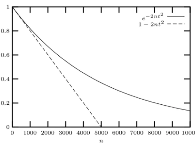
−ε probability an ap-1e−2nt2 −2nt2 n 10000 9000 8000 7000 6000 5000 4000 3000 2000 1000 0 1 0.8 0.6 0.4 0.2 0
Figure 1: Upper bound on the probability that the computed probability exceeds the real value by more thant, for t = 0.01. −logt2t t log 10 scale 0.1 0.08 0.06 0.04 0.02 0 7 6.5 6 5.5 5 4.5 4 3.5 3 2.5 2
Figure 2: Numbers of iterations necessary to achieve a prob-ability of false report on the same order of magnitude as the error margin.
proximation of the requested probabilityµ, it is sufficient to compute an experimental average over −log2t2ε trials.
This exponential improvement in quality (Fig. 1) is nev-ertheless not that interesting. Indeed, in practice, we might want εand tof the same order of magnitude as µ. Let us take ε = αt where α is fixed. We then have n ∼ −logt
t2 , which indicates prohibitive computation times for low prob-ability events (Fig. 2). This high cost of computation for low-probability events is not specific to our method; it is true of any Monte-Carlo method, since it is inherent in the speed of convergence of averages of identically distributed random variables; this relates to the speed of convergence in the cen-tral limit theorem [14, ch 1]. It can nevertheless be circum-vented by tricks aimed at estimating the desired low prob-ability by computing some other, bigger, probprob-ability from which the desired result can be computed.
Fortunately, such an improvement is possible in our method. If we know thatπ1([[c]]−1(W))⊆R, with a mea-surableR, then we can replace the random variable tW by
its restriction to R: tW|R; then EtW = Pr (R).EtW|R. If
Pr (R) and EtW are on the same order of magnitude, this
means that EtW|R will be large and thus that the number
of required iterations will be low. Such a restricting Rcan be obtained by static analysis, using ordinary backwards ab-stract interpretation.
A salient point of our method is that our Monte-Carlo computations arehighly parallelizable, with linear speed-ups: niterations on 1 machine can be replaced byn/m iter-ations onmmachines, with very little communication. Our method thus seems especially adapted for clusters of low-cost PC with off-the-shelf communication hardware, or even more distributed forms of computing. Another improvement can be to compute bounds for severalWsets simultaneously, doing common computations only once.
5
PRACTICAL IMPLEMENTATION
AND EXPERIMENTS
We have a prototype implementation of our method, imple-mented on top of an ordinary abstract interpreter doing for-ward analysis using integer and real intervals. Figures 3 to 5 show various examples for which the probability could be computed exactly by symbolic integration. Figure 6 shows a simple program whose probability of outcome is difficult to figure out by hand. Of course, more complex programs can be handled, but the current lack of support of user-defined functions and mixed use of reals and integers prevents us from supplying real-life examples. We hope to overcome these limitations soon as implementation progresses.
6
CONCLUSIONS
We have proposed a generic method that combines the well-known techniques of abstract interpretation and Monte-Carlo program testing into an analysis scheme for probabilis-tic and nondeterminisprobabilis-tic programs, including reactive pro-grams whose inputs are modelized by both random and non-deterministic inputs. This method is mathematically proven correct, and uses no assumption apart from the distributions and nondeterminism domains supplied by the user. It yields
int x, i; know (x>=0 && x<=2); i=0; while (i < 5) { x += coin_flip(); i++; } know (x<3);
Figure 3: Discrete probabilities. The analyzer es-tablishes that, with 99% safety, the probability p of the outcome (x < 3) is less than 0.509 given worst-case nondeterministic choices of the precondition (x≥0∧x≤2). The analyzer usedn= 10000 random trials. Formally,pis
Prcoin flip∈ {0,1}5| ∃x∈[0,2]∩
[[P]](coin flip, x)<3. Each coin flip is chosen randomly in {0,1} with an uniform distribution. The exact value is0.5.
double x;
know (x>=0. && x<=1.);
x+=uniform()+uniform()+uniform(); know (x<2.);
Figure 4: Continuous probabilities. The analyzer es-tablishes that, with 99% safety, the probability p of the outcome (x <2) is less than0.848given worst-case nonde-terministic choices of the precondition (x ≥ 0∧x ≤ 1). The analyzer used n = 10000 random trials. Formally,
p is Pruniform∈[0,1]
3
| ∃x∈[0,1] [[P]](uniform, x)<2 . Eachuniformis chosen randomly in [0,1] with the Lebesgue uniform distribution.
The exact value is 5/6≈0.833.
double x, i; know(x<0.0 && x>0.0-1.0); i=0.; while (i < 3.0) { x += uniform(); i += 1.0; } know (x<1.0);
Figure 5: Loops. The analyzer establishes that, with 99% safety, the probability p of the outcome (x <
1) is less than 0.859 given worst-case nondeterministic choices of the precondition (x < 0 ∧x > −1). The analyzer used n = 10000 random trials. Formally,
p is Pruniform∈[0,1]
3
| ∃x∈[0,1] [[P]](uniform, x)<1 . Eachuniformis chosen randomly in [0,1] with the Lebesgue uniform distribution. The exact value is 5/6≈0.833.
{ double x, y, z; know (x>=0. && x<=0.1); z=uniform(); z+=z; if (x+z<2.) { x += uniform(); } else { x -= uniform(); } know (x>0.9 && x<1.1); }
Figure 6: The analyzer establishes that, with99% safety, the probability p of the outcome (x > 0.9 ∧x < 1.1) is less than 0.225 given worst-case nondeterministic choices of the precondition (x≥0∧x≤0.1). Formally,pis Pruniform∈[0,1]
2
| ∃x∈[0,0.1] [[P]](uniform, x)∈[0.9,1.1] . Eachuniformis chosen randomly in [0,1] with the Lebesgue uniform distribution.
upper bounds on the probability of outcomes of the program, according to the supplied random distributions, with worse-case behavior according to the nondeterminism; whether or not this bounds are sound is probabilistic, and a lower-bound of the soundness of those bounds is supplied. While our ex-planations are given using a simple imperative language as an example, the method is by no means restricted to imper-ative programming.
The number of trials, and thus the complexity of the com-putation, depends on the desired precision. The method is parallelizable with linear speed-ups. The complexity of the analysis, or at least its part dealing with probabilities, in-creases if the probability to be evaluated is low. However, static analysis can come to help to reduce this complexity.
We have implemented the method on top of a simple static analyzer and conducted experiments showing interesting re-sults on small programs written in an imperative language. As implementation progresses, we expect to have results on complex programs akin to those used in embedded systems.
REFERENCES
[1] Patrick Cousot and Radhia Cousot. Abstract interpre-tation and application to logic programs.J. Logic Prog., 2-3(13):103–179, 1992.
[2] Patrick Cousot and Nicolas Halbwachs. Automatic dis-covery of linear restraints among variables of a program. InProceedings of the Fifth Conference on Principles of Programming Languages. ACM Press, 1978.
[3] Jifeng He, K. Seidel, and A. McIver. Probabilistic mod-els for the guarded command language.Science of Com-puter Programming, 28(2–3):171–192, April 1997. For-mal specifications: foundations, methods, tools and ap-plications (Konstancin, 1995).
[4] Wassily Hoeffding. Probability inequalities for sums of bounded random variables. J. Amer. Statist. Assoc., 58(301):13–30, 1963.
[5] Alexander S. Kechris. Classical descriptive set theory. Graduate Texts in Mathematics. Springer-Verlag, New York, 1995.
[6] D. Kozen. Semantics of probabilistic programs. In20th Annual Symposium on Foundations of Computer Sci-ence, pages 101–114, Long Beach, Ca., USA, October 1979. IEEE Computer Society Press.
[7] D. Kozen. Semantics of probabilistic programs. Journal of Computer and System Sciences, 22(3):328–350, 1981. [8] N. G. Leveson. Software safety: Why, what, and how.
Computing Surveys, 18(2):125–163, June 1986. [9] David Monniaux. Abstract interpretation of
probabilis-tic semanprobabilis-tics. InSeventh International Static Analysis Symposium (SAS’00), number 1824 in Lecture Notes in Computer Science. Springer-Verlag, 2000.
[10] Carroll Morgan, Annabelle McIver, Karen Seidel, and J. W. Sanders. Refinement-oriented probability for CSP. Formal Aspects of Computing, 8(6):617–647, 1996.
[11] Simeon Ntafos. On random and partition testing. In Michal Young, editor, ISSTA 98: Proceedings of the ACM SIGSOFT International Symposium on Software Testing and Analysis, pages 42–48, 1998.
[12] Panel on Statistical Methods in Software Engineering. Statistical Software Engineering. National Academy of Sciences, 1996.
[13] H. Rogers.Theory of recursive and effective computabil-ity. MGH, 1967.
[14] Galen R. Shorack and Jon A. Wellner. Empirical Pro-cesses with Applications to Statistics. Wiley series in probability and mathematical statistics. John Wiley & Sons, 1986.
[15] P. Th´evenod-Fosse and H. Waeselynck. Statemate ap-plied to statistical software testing pages 99-109. In Pro-ceedings of the 1993 international symposium on Soft-ware testing and analysis, pages 99–109. Association for Computer Machinery, June 1993.