Combining Control and Data Abstraction in the
Verification of Hybrid Systems
Xavier Briand and Bertrand Jeannet
Abstract—This paper addresses the verification of hybrid systems built as the composition of a discrete software controller interacting with a physical environment exhibiting a continuous behavior. The goal is to attack the problem of the combinatorial explosion of discrete states that may happen if a complex software controller is considered. It proposes as a solution to extend an existing abstract interpretation technique, namely dynamic par-titioning, to hybrid systems described in a symbolic formalism. Dynamic partitioning allows us finely tune the tradeoff between precision and efficiency in a reachability analysis. It shows the effectiveness of the approach by a case study that combines a nontrivial controller specified in the synchronous dataflow programming language Lustre with its physical environment.
Index Terms—Abstract interpretation, hybrid systems, logico-numerical properties, synchronous languages verification.
I. Introduction
H
YBRID SYSTEMS have the particularity to combinea discrete behavior, specified with traditional test and assignment operations, with a continuous behavior, specified by the mean of differential equations or inclusions. They primarily allow us to model a physical environment ruled by physical laws, which may be either purely continuous, or mixing discrete and continuous aspects (like a bouncing ball). Hybrid systems are also particularly well-suited to model the behavior of a software controller that exhibits a discrete behavior, interacting with a physical environment ruled by physical laws. Such systems have recently been given the name ofcyberphysical systems.
This paper targets specifically this latter case, and is mo-tivated by the problem of analysing a Lustre synchronous program interacting with a physical environment. Lustre
[23] is a domain-specific dataflow language for programming control-command systems that periodically sample inputs from their environment, compute outputs and move to a new internal state. When verifying properties on such programs, it is mandatory to take into account a reasonably accurate model of their physical environment, as these programs make assump-tions on their environment. For instance, a speed regulation system implicitly assumes that when it orders an acceleration,
Manuscript received December 16, 2009; revised April 10, 2010; accepted May 19, 2010. Date of current version September 22, 2010. This paper was recommended by Associate Editor R. Bloem.
The authors are with INRIA-Grenoble, Rhˆone-Alpes, Montbonnot Saint Martin 38334, France (e-mail: [email protected]; bertrand. [email protected]).
Color versions of one or more of the figures in this paper are available online at http://ieeexplore.ieee.org.
Digital Object Identifier 10.1109/TCAD.2010.2066010
the speed should increase. The resulting combination of a program and its environment is a hybrid system, that has usually the specificity of having a large discrete state-space, inherited from the state-space of the controller program.
Verification of hybrid systems focuses, however, mainly on the analysis of the continuous behavior; the values of
non-numerical variables are encoded in the control structure. Invariants for numerical variables are then defined for each
corresponding control point, as illustrated in Fig. 1(a). This may result in a combinatorial explosion of the number of control points, a well-known problem in the verification of finite-state systems. Moreover, compared to the case of purely discrete systems, hybrid systems make this combinatorial explosion even more difficult to tackle because invariants are more complex properties (e.g., convex polyhedra) rather than a boolean value (indicating that a state is or is not reachable).
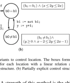
The aim of this paper is to tackle this combinatorial explo-sion problem by extending the principle ofdynamic partition-ingto hybrid systems [29], [30]. The initial motivation for this technique, based on abstract interpretation, was to apply linear relation analysis [16], [25] to dataflow synchronous programs manipulating Boolean and numerical variables. The idea is to consider more general and less detailed control structures, such as the one depicted in Fig. 1(b). Fig. 1 illustrates the less precise invariants obtained by the analysis if we merge the locations according to the propertyb0 = b1.
The term “dynamic” refers to the ability of incrementally refiningsuch a control structure in order to reach a sufficient precision for the verification goal. The refinement is performed in conjunction with a combination of forward and backward analyses, so that only states that potentially belong to a counter-example are considered in the refinement process.
A. Existing Approaches for Verifying Hybrid Systems
Since the first papers on the verification of such systems [2], [24], [27], the approaches based on the use of convex polyhedra and on the resolution of fixpoint computations are still of interest. Convex polyhedra are indeed able to infer
subtle relationship between the variables of a system [15]. An obvious limitation of convex polyhedra is that they cannot provide good approximations of non convex invariants. The
HyTech tool [26] solves this problem by using unions of convex polyhedra, but it results a possibly non-terminating (and more costly) analysis, unlike the abstract interpretation approach of [25]. As an alternative, [5] and [6] suggest approximating subsets ofRnwith unions of hypercubes, using 0278-0070/$26.00 c!2010 IEEE
Fig. 1. Associating invariants to control location. The boxes formula give the invariant computed for each location with a linear relation analysis. (a) Fully explicit control structure. (b) Partially explicit control structure.
efficient algorithms. A strength of this method is the ability to have canonical representation of non-convex sets and to handle more complex differential equations. However, a combinato-rial explosion of the numbers of hypercubes quickly arises. Ellipsoid methods have also been proposed [32]. Presented as a successor of HyTech, thePHAvertool offers sophisticated refinement techniques for representing non-convex invariants by unions of polyhedra and for approximating on-the-fly linear differential equations by simpler piecewise-constant dral inclusions that can be treated directly with convex polyhe-dra. Convergence of computations can be achieved by various heuristics.
As mentioned in [17],HyTechandPHAverfail when deal-ing with large discrete space because only continuous behav-iors are treated symbolically. [17] proposes a fully symbolic technique based on backward (greatest) fixpoint computation, in which sets of states are represented exactly with a vari-ant of Boolean circuits mixing Boolean variables and linear constraints. The technique does not guarantee termination (on unbounded time intervals), and relies on a sophisticated semi-canonical representation rather than on approximations to ad-dress the efficiency issue. In the case of discrete systems, [11] adopts a similar approach by combining binary decision dia-grams (BDDs) and Presburger formulas in disjunctive normal
forms.
Methods based on predicate abstraction will be discussed later in Section IV.
All the above-mentioned methods are based on reachable state exploration. Another approach, mostly applied to discrete systems until recently, exploits the power of modern satisfia-bility (SAT) and satisfiasatisfia-bility modulo theory (SMT) solvers to perform two different tasks:
1) finding counter-examples of some length k ≤ K, by
encoding this problem as a (generalized) SAT problem;
2) proving properties by induction of order k, which
con-sists of proving that if a property is true for any k
consecutive execution steps, it is true for the stepk+ 1
(in addition to the corresponding base case that considers the initial states).
Reference [18] applies (1), in the particular case of hybrid systems with rectangular constant inclusion, which is less general than our model. Technique (2) is not complete, in particular because it does not take into account reachability information, but it can be very efficient in practice (see [22] for its application to discrete Lustre programs). We are not aware of an application ofk-induction to hybrid systems.1
B. Contribution
We present here a reachable state analysis that combines efficiently discrete and continuous behavior for the verification of hybrid systems obtained as the composition of a physi-cal environment and a software controller, as illustrated in Section II.
To implement our idea, we need a higher-level model for hybrid systems.
1) We should be able to embed dataflow Lustreprogram in our model.
2) We also need a more symbolic model, as a key point of our technique is to handle symbolically both the discrete and the continuous part of the state-space.
From a specification point of view, we thus propose in Section III a flexible model for hybrid systems which is more symbolic in a number of aspects. Some usual constraints are relaxed, like the requirement that invariants and guards should be convex. One can also combine freely numerical and non-numerical variables in formulas, as in Lustre programs, and we propose an original way to specify more concisely continuous behaviors, in particular by specifying with a sin-gle formula both continuous invariants and constraints on derivatives.
Section IV reminds the principles of dynamic partitioning developed in [29]. In this context, Section V extends these principles to hybrid systems, by defining a suitable method for computing continuous post and preconditions induced in a partitioned abstract domain. Integrated in our tool NBac, this extension allows us to inherit the features of dynamic partitioning for hybrid systems.
We last illustrate in Section VI with experiments the po-tential of our approach. We first performed various analyses on the example presented in Section II, and we then tackled a very detailed model of the famous steam-boiler specification of Abrial [1]. Such a system could hardly be handled with-out treating symbolically the discrete state-space, due to the complexity of its discrete behavior.
Our original contributions are located in Sections III, V, and VI. This paper is a journal version of [10], with some material considered as not essential removed and other mate-rial explained with more details and examples.
II. Connecting aLUSTRE Program to a Hybrid Environment
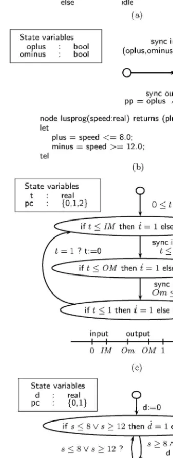
Fig. 2 shows a model of a system composed of a Lus-tredisk controller interacting with its physical environment, namely a disk motor device (hybrid system). Fig. 2(a) depicts the behavior of the disk motor. It emits its speed on theinput
channel, and obeys to the command received with theoutput
channel, but may diverge slightly from the ideal behavior (parameter!).
Fig. 2(b) depicts the disk controller. It receives the speed of the disk and emits appropriate signals plus and minus
to maintain the motor speed within a specified range (here the interval [8,12]). This program is embedded in a hybrid
automaton which receives the speed on the channel input, computes the reaction of theLustrecontroller and stores the computed outputs in internal variables, before emitting them on channeloutput.
The process of Fig. 2(c) forces the synchronizations on channels input and output to take place in the right order, within specific time intervals. We model thus the reaction time of the controller, and variations in the sampling period and the reaction time. The parameters are!, m, M,IM,Om,OM.tis
a local clock used for measuring delays, andpcis the implicit program counter that encodes the three locations (we dot not have explicit control location in our formal model presented in Section III, although we use them in graphical descriptions).
Fig. 2(d) depicts the property observer.dis the time during which the speed has been outside the interval [8,12]. We want
to check if d ≤ 8 always holds. As initially the speed is 0,
the controller should put the motor speed in the desired range quickly enough, and control it properly afterward.
III. Symbolic Hybrid Automata (SHA)
We introduce in this section a symbolic model for hybrid systems, which allows us to manipulate symbolically locations and location invariants, and which is actually used in Fig. 2. Thus, we can avoid the state-explosion problem in the speci-fication and delay this issue to the analysis.
From a computational point of view, the expressiveness of SHA is identical to linear hybrid automata. However, from a specification language point of view, SHA are more expressive in so far as they allow much more compact descriptions.
A. SHA Model
A SHA H = (V,Init, "H, DH) is defined by a set V
of variables evolving from initial state Init according either to discrete and instantaneous changes (with assignments) specified by"H, or tocontinuous evolutionsspecified with a
global,conditional differential inclusionDH. More precisely:
1) V is a finite set of variables partitioned into variables of
any type inVQ (subject to discrete behaviors only) and
real-valued variables inVX.Q(resp.X) denotes the set
of valuations of variables inVQ (resp.VX).S=Q×X
is the set of states of the system andInit⊆S the initial
states.
Fig. 2. Disk controller connected to its environment, and a property observer. (a) Environment: disk motor device emits the speed of the disk on channel input and reacting to the controller (channel output). (b) LUSTRE controller embedded in a process. It emitsplusandminuscommands to the physical device. (c) Scheduler defining the scheduling above. (d) Property observer on the physical environment: d counts the delay for which the speed s has been outside the desired range.
Fig. 3. Formal definition of the SHA of Fig. 2(a).
2) Discrete changes of the system are defined by a finite set "H of transitions. In a discrete transition δ =
(σ, p, G, A)∈"H:
a) σ is achannelcarrying a tuple ofcommunication parametersp=%p1, . . . , pk&;
b) the guard G ⊆ S ×Pσ is a predicate on the
variables and the communication parameters (Pσ
denotes the set of valuations of parameters);
c) the assignment A : S ×Pσ → S defines the
evolution of the values of variables during the discrete transition.
For instance, in Fig. 2(a) the transition labeled by the
outputchannel is defined byσ=output,p=%pp,mm&,
G= true, and Aassigns the variable mode depending on the communication parameterspp,mm, and leaves the
other state variables unchanged.
3) The continuous evolution is defined by a functionDH : Q×X→2Xthat associates with each discrete stateq∈ Q adifferential inclusionx˙(t)∈DH(q, x(t)). Examples
of differential inclusions DH are [if b then dx = dy +1 else dx = dy] or [if x> =2then dx = dy +1else dx = dy].
For instance, Fig. 3 gives the formal definition of the SHA depicted in Fig. 2(a).
We detail some key differences of our model compared to the “classical” model of hybrid automata most often consid-ered in the verification community [2], [19].
1) It does not restrict a priori the types of the discrete variables in VQ, as the software controller part may
manipulate variables of various types (integers, floating-point numbers, and so on).
2) It does not use explicit locations or control points; these need to be encoded withprogram countervariables. This enables us to play with the control structure, as shown in Fig. 1.
3) The constraints DH on the derivatives of continuous
variables are a function on all state variables rather than a function on discrete locations only.
4) The classical model uses the notion oflocation invariant
to partially solve the non-determinism between the time elapse and the firing of a discrete transition. A location invariant is a predicate on continuous variables that must be true for the time to elapse, and that forces a discrete transition to be taken when it becomes false. For instance, in Fig. 5(a) the constraint 1≤ x≤3 is
a location invariant that must be true for x to evolve
according to the differential equationx˙=x. In our model
location invariants are implicitly defined by (the guards
of) the differential inclusion functionDH, as explained
below.
Let us illustrate by a few examples points 3 and 4. The differential inclusion [if b then dx = dy + 1 else dx = dy] uses the Boolean variable b to encode two traditional locations with the universe as invariant [see also Fig. 2(a)]. The differential inclusion [if x> = 2 then dx = dy +
1 else dx = dy] specifies two traditional locations with invariantsx≥2 (resp.x <2) and differential inclusionsx˙ =y˙+1
(resp.x˙ =y˙), with an implicit discrete transition between them
when x = 2; trajectories may cross the frontier of the two
connex regions. [if x <=3 then dx = 1 else empty] is our way to specify a traditional location with differential equation
˙
x= 1 and invariant x≤3; when x >3, there are no possible
valuations for the derivatives (DH =∅), hence the time cannot
elapse any more.
SHAs can be composed in parallel and communicate by
rendez-vous on valued channels. When a synchronization takes place on a channel σ(p), all the involved SHAs should
agree on the value of the communication parameters p. The
corresponding product, used in Fig. 2, is classical and is not detailed here. Notice that once SHAs are composed in parallel, in the resulting product SHA the synchronizations on valued channels are still meaningful, because they introduce “input” communication parameters that may be constrained by the guard and used in the assignment of a transition. Stated differently, they allow us to model opened systems receiving (possibly constrained) inputs from their environments.
1) Syntax of Expressions: In our verification tool, functions involved in the definition of hybrid automata are functions that can be put under the form defined by the grammar of Fig. 4. For instance
dx1 = (if b1 then1else 0) and dx2 = (if b2 then1else 0)
can be rewritten as if b1
then (if b2 then dx1 = dx2 = 1 else dx1 = 1 and dx2 = 0)
else (if b2 then dx1 = 0 and dx2 = 1 else dx1 = dx2 = 0)
which belongs to this grammar.
Such functions are internally represented with binary de-cision diagrams (multiterminal BDDs,MTBdds, [9]) built on atomic decisions (Boolean variables or linear constraints) and elementary functions, as in [28]. For elementary differential inclusions, denoted in Fig. 4 by the non-terminal “%diffcons&,” in this paper we consider only linear hybrid automata, that is, hybrid systems with constant and closed differential inclusion (conjunction of non-strict linear constraints on derivatives, like 1 ≤ ˙x+ 2y˙ ≤ 3). This excludes affine differential equations
of the form x˙ = x. They can however be approximated by
piecewise constant differential inclusions. Notice that a few tools like PHAVer internally perform such approximations.
B. Behavior of SHA
Therunof a SHAHis composed of a succession of discrete
and continuous transitions. The global transition relation is →=→c∪ →d is defined as follows.
Fig. 4. Syntax of normalized expressions in SHA.
1) Discrete Transition Relation: The discrete transition relation→d⊆S×S induced by "H is defined by
(σ, p, G, A)∈"H, vp ∈Pσ, (s, vp)∈G∧s,=A(s, vp) s→d s,
.
2) Continuous Transition Relation: We denote byFT the
set of functionsf : [0, T]→X piecewiseC1, i.e., there is a
finite sequence T0 = 0 < T1 < . . . < Tn = T such that f is
continuously differentiable on ]Ti, Ti+1[ and has a left limit in Ti and a right limit inTi+1. The continuous transition relation
→c⊆S×S induced by the conditional differential inclusion DH is defined by
q∈Q, T ≥0, f ∈FT, f(0) =x∧f(T) =x,
∀i < n, ∀t∈]Ti, Ti+1[:f˙(t)∈DH(q, f(t)) s= (q, x)→cs,= (q, x,)
. (1)
Remark that if DH(s) = ∅, there is no possible continuous
transition from s, so the time cannot elapse any more, and
only discrete transitions can possibly be taken. This allows to implement the traditional notion of invariants as explained in Section III-A. The linear hybrid automata defined in [2] are SHA where the valuations of discrete variablesQare the
locations, and where DH(q, x) = ifx ∈ Iq thenCq else ∅,
with the invariant Iq and condition on derivatives Cq are
convex polyhedra.
We introduce also few additional notations, used below for reachability analysis. Given a discrete state q we call T
-trajectories the functions ν : [0, T] → S such that ν(t) =
[q, f(t)] and we denote by TT the set ofT-trajectories. The
postcondition and precondition operatorspost,pre: 2S
→2S
are defined as
post(X) ={s, |s∈X∧s→s,} (2) pre(X) ={s| s,∈X∧s→s,}. (3)
For a monotone function F : L → L where L is a lattice,
lfp(F) denotes the least solution of the fixpoint equationX= F(X). States reachable for an initial setI ⊆Sor coreachable
from a final setF ⊆S can be characterized by the following
fixpoint equations on the lattice (2S,
⊆):
reach(I) = lfp(λX.I∪post(X)) (4) coreach(F) = lfp(λX.F∪pre(X)). (5)
As we focus in this paper only on (co)reachability proper-ties, we are not concerned with some pathological behavior
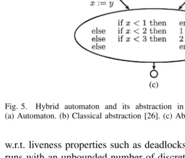
Fig. 5. Hybrid automaton and its abstraction in two different models. (a) Automaton. (b) Classical abstraction [26]. (c) Abstraction with SHA.
w.r.t. liveness properties such as deadlocks or Zeno runs (i.e., runs with an unbounded number of discrete transitions within a bounded time interval). Our analysis method still returns sound results in such cases.
C. Discussion
Although the primary motivation for our symbolic model is to implement the ideas developed in the introduction re-garding symbolic verification techniques, we think it is a very interesting model for its expressiveness and compactness.
For instance, the automaton of Fig. 5(a) can be abstracted by the automaton of Fig. 5(b). This requires however the duplication of discrete transitions, sometimes with guards modifications (incoming transitions), whereas our model en-ables a more straightforward specification of the abstraction [Fig. 5(c)]. In the same way, in Fig. 2(a), we do not need to specify explicitly the discrete transitions between the different continuous modes defined according to the value of variable
mode. Fig. 2(d) illustrates the ability to specify with the same formula both the location invariant and the constraints on derivatives, and the possibility to have non-convex invariants. In this respect, our SHA model is higher-level than the classical models considered in [2] and in theHyTech or the
PHAververification tools. However, it is still a mathematical model in the sense that it remains automaton-based and it does not offer modeling constructs such as the χ hybrid process
algebra [8], [38].
If we look now to models mainly dedicated to simulation, likeSimulink[35] orModelica, [34] the picture is different. On the one hand, in those models both the discrete and the continuous behavior may be specified in a very general way, using for instance C functions. On the other hand, simulation models forbid (implicit) non-deterministic choices between leaving the time elapse or firing discrete transitions. They thus replace the notion of (location) invariant by the notion of zero-crossings, which are numerical expressions given to
the numerical integration solver. The solver will stop the integration process as soon as one of these expressions crosses zero from below and changes its sign. When this happens, the solver gives the hand back to the discrete simulator, which then fires the discrete transition guarded by the activated zero-crossing.
For verification purposes however, location invariants or guarded differential inclusions as in our case are more ade-quate for symbolically computing the effect of time elapse.
IV. Abstract Interpretation and Dynamic Partitioning
We want to check an invariance property on a hybrid system, or equivalently to show that some states cannot be reached. If
BAD⊆S denotes such states, we expect
reach(Init)∩BAD=∅ or coreach(BAD)∩Init=∅.
As the sets reach and coreach are not computable for the considered systems, we will use approximation techniques of [29] based on abstract interpretation [14].
A. Base Abstract Domain
The idea of abstract interpretation is to replace the powerset of states (2S,
⊆) partially ordered by inclusion [on which (4) and (5) are defined] by a simpler abstract lattice (A,/) in
order to achieve reasonable performance of the resulting ab-stract analysis, without being too imprecise either. An abab-stract domain may be seen as a class of geometrical shapes that enjoy nice properties w.r.t. their expressiveness and the complexity of the operations on them. The meaning of anabstract value a∈Ais given by aconcretization function γ:A→2S such
that a1/a2 ⇔γ(a1)⊆γ(a2).
For instance, if S= Rm, one can replace 2S by theconvex polyhedra abstract domain Pol(Rm). As convex polyhedra
are just specific subsets of Rm, γ is just the identity. The
abstraction comes from the fact that the set union∪which is the least upper bound of the lattice (2S,
⊆) is approximated by the convex hull 1C which is the least upper bound of the lattice (Pol(Rm),
⊆).
In our particular case, a concrete value is a subset of the state-spaceS2Bn
×Rm (enumerated variables
×numerical variables). Here we make the choice that an abstract value
a= (B, P) ∈ A= 2Bn×Pol(Rm) (6)
is the conjunction of a Boolean formulaB (represented with
a BDD) and an m-dimensional convex polyhedron P. The
concretization functionγ:A→2Sand the least upper bound
1are defined by
γ(B, P) ={(b, x)∈S | b∈B∧x∈P} (7)
(B1, P1)1(B2, P2) = (B1∨B2, P11CP2). (8)
Such an abstract domain forgets the relations between vari-ables of different types, which is a quite rough approximation.
For instance, one cannot represent the relation (b0⇔x0≥0),
because (b0, x0 ≥0) 1(¬b0, x0 <0) = (true,R) according
to (8).
An alternative could be to consider the much more precise abstract domain
A,=Bn→Pol(Rm) (9)
with
γ,(f ∈A,) ={(b, x)| x∈f(b)} (10) f11,f2=λb . f1(b)1Cf2(b) (11)
in which a convex polyhedra is associated with each discrete state, which allows us to represent accurately a relation like (b0 ⇔ x0≥0). This solution does not address however the
combinatorial explosion problem. More generally, none of these two solutions can represent non-convex invariants for numerical variables.
1) Solving Fixpoint Equations on an Abstract Domain:
We remind that we want to solve the fixpoint (4) and (5). The transfer fixpoint theorem says that ifFα:A→Ais acorrect approximationofF : 2S→2S, which means thatγ◦Fα⊇F◦ γ, thenγ◦lfp(Fα)⊇lfp(F). In other words, a fixpoint equation X = F(X), X∈ 2S can be abstracted by Y = Fα(Y), Y ∈A,
and the least solutionY0= lfp(Fα) overapproximates the exact
setX0= lfp(F).
IfFαis continuous andAis a complete lattice that contains
no infinitely increasing sequences, the most classical way to compute lfp(Fα) is to compute the sequence
Y(0)=⊥, Y(n+1)=Fα(Y(n)) (12)
which converges in a finite number of steps to lfp(Fα)
ac-cording to Kleene’s theorem. Otherwise, if A is not
com-plete and/or contains infinitely increasing sequences (as for instance the convex polyhedra lattice), in addition to thestatic approximation induced by the abstract lattice, one introduces a dynamic approximation by using an extrapolation operator ∇ :A×A→Acalledwidening[14]. Equation (12) is replaced
by
Y(0)=⊥, Y(n+1)=Y(n)∇Fα(Y(n)) (13)
which converges in a finite number of steps to apost-fixpoint Y 8Fα(Y)
8lfp(Fα) thanks to technical properties of
∇.2
The aim of abstract interpretation framework is thus to generalize the intuitive approximation of geometrical shapes (for instance by bounding boxes or convex polyhedra) to the approximation of more complex objects encountered in program analysis. An important point to be noticed is that in numerical analysis, the notion of approximation is based on the notion of topological neighborhoods, whereas in program analysis and abstract interpretation, it is based on set inclusion.
2The use of widening solves in particular problems related to Zeno behavior
B. Partitioned Abstract Domain
We already mentioned the shortcomings of the two abstract domains A and A, we defined for 2S [(6) and (9)] w.r.t.
precision and efficiency.
A flexible solution to these problems is to partition the efficient but not very precise abstract domain A in order to
improve its expressiveness. Intuitively, partitioning allows us to introduce case reasoning by distinguish different situations and by manipulating disjunctions. For instance, if we partition
Aaccording to an inequalityx≥10, we can represent exactly
an invariant like ⊆ x≥10 ! "# $ (b, x≥20) ∪ ⊆x<10 ! "# $ (true,−10≤x≤0) (14)
whereas a single abstract value inAcan only approximate the
above invariant with (true,−10≤x).
More formally, ifπ={A1, . . . , An} ⊆Ais a finite set such
that {Sk = γ(Ak) | 1≤k≤n} defines a finite partition of S,
then we can define the abstract domainAπ ={(a1, . . . , an)∈ An | ak / Ak}. Its concretization function and least upper
bound are defined as
γπ(a1, . . . , an) =γ(a1)∪. . .∪γ(an)
(a1, . . . , an)1π(a,1, . . . , a,n) = (a11a,1, . . . an1a,n).
This allows us to manipulate bounded and canonical unions of abstract values, and in particular to represent non-convex numerical invariants, as in (14).
To reflect the partitionπin (4), we first exploit the
isomor-phism 2S≈2S1×. . .×2Sn to rewrite the reachability fixpoint
equationX=I∪post(X) as Xk=Ik∪% k, postk,,k ! "# $ (post(Xk,)∩Sk)(Xk,) (15) withXk, Ik⊆Sk and 1≤k≤n. We then abstract it with
Yk=Yk(0)1 &
k,
postαk,,k(Yk,) (16) where γ(Yk(0) ⊇ Ik and postk,,k
α : A → A is a correct
approximation of postk,,k : Sk, → Sk. The abstract interpre-tation framework ensures that we can compute iteratively the reachability set in the partitioned abstract domain Aπ using
widening. We obtain an overapproximation reach+
⊇ reach of the concrete reachability set. Fig. 1 illustrates two possible partitioning ofS=B2×R2, according either to all the Boolean
variables, or to the conditionb0=b1, and the corresponding
reachability analyses.
C. Partition Refinement
The more the partitionπis detailed, the more the abstraction Aπ is precise, but also costly. The idea of [29], illustrated in
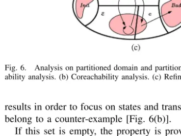
Fig. 6, is then to start with a simple partition, to perform reachability and coreachability analysis, and to intersect their
Fig. 6. Analysis on partitioned domain and partition refinement. (a) Reach-ability analysis. (b) CoreachReach-ability analysis. (c) Refinement.
results in order to focus on states and transitions that possibly belong to a counter-example [Fig. 6(b)].
If this set is empty, the property is proved. Otherwise, we refine the partition and start a new analysis cycle. Contrary to most predicate abstraction refinement techniques, that are based on the search of concrete counter-examples [3], our refinement technique can be viewed as based on abstract counter-examples, that is, it tries to remove paths from initial to bad states. In a partition member, a condition [like the condition cin Fig. 6(b)] that separates different behaviors (in
terms of abstract transitions) is a good candidate for partition refinement, as it allows us to remove some transition paths in the partition. For instance, the refinement depicted in Fig. 6(c) makes clear that one cannot go in one step from the partition member labeled by ¯c to the bad states, something which
appeared as possible in Fig. 6(a).
Reference [29] proposes several refinement heuristics on this basis. Necessary conditions to jump from one partition member to another one (like the condition c in Fig. 6) are
naturally obtained as a side effect of the technique described in Section V for computing postconditions.
1) Dynamic Partitioning and Predicate Abstraction: Pred-icate abstractionconsists of abstracting a (hybrid) system with an abstract finite automaton, by partitioning the state-space of the original system according to a set of formulas, and then abstracting accordingly its transition relation [21]. The abstract system is then checked by classical finite-state exploration techniques. As the choice of a suitable partition is of crucial importance (as in dynamic partitioning), refinement techniques have been developed, both for non-hybrid or hybrid cases [3], [12], [27], based on concrete counter-examples or the notion of interpolants [33]. Predicate abstraction can be seen as an instance of dynamic partitioning, where the base abstract domain is the simple lattice{⊥,;}with⊥ ! ;; the fixpoint
computation on the abstract finite automaton can only show that an abstract state is either non-reachable (⊥) or possibly reachable (;). In contrast, dynamic partitioning makes use of more sophisticated abstract domains like convex polyhedra [30], which allows a full range of properties lying between⊥ and;to be discovered by the fixpoint computation.
In some intuitive way, the “cleverness” of predicate abstrac-tion is mainly located in the generaabstrac-tion of a detailed partiabstrac-tion by the refinement process, whereas dynamic partitioning relies less on a detailed partitioning and more on propagation of symbolic properties during fixpoint computations. In particu-lar, in our method we forbid the refinement process to split the state-space according to a condition (Boolean variable or numerical constraint) that does not appear in the program. The main motivation is that we do not want to start enumerating the value of a counteri= 0,i= 1,. . . in the partition, something
which can happen with some predicate abstraction refinement techniques, and which is much less useful in our case, as our fixpoint computations can discover new facts in a non-finite, more expressive abstract domain.
As a side-effect, our refinement process is guaranteed to terminate, leading to a finite partition such that the transition functions partially evaluated on each partition member do not contain conditions any more (according to the syntax of Fig. 4). However, there is no guarantee that the property is provable on the corresponding partitioned abstract domain.
V. Computing Continuous Postconditions
Section III presented our SHA model and Section IV presented our general approach to compute reachable states of such systems. To instantiate it, we need to compute the operatorpostk,,k
α appearing in (16), which is a correct
approx-imation of the operator λX ⊆ Xk,.'post(X)∩Xk
(. As the
transition relation of a SHA has been defined in Section III-B as the union of a discrete and continuous transition relations, we can decompose the postcondition operatorpostdefined by (2) as the union of adiscreteand acontinuouspostcondition operators. A method for efficiently computing the discrete postcondition operator is described in [28], so we will focus only on the computation of continuous postconditions.
In classical linear hybrid automata defined in [2], computing a continuous postcondition is quite straightforward; a change of mode requires a discrete transition, and in each mode the constraints on derivatives are constant; only trajectory segments that are line segments need to be considered. Our framework introduces two difficulties.
1) In the SHA model a change of mode can occur during continuous evolutions; the trajectory segments to con-sider are more complex and the induced postcondition should sometimes be approximated. Moreover, the topo-logical aspects on the frontier separating two partition members have to be taken into account carefully. 2) We must take into account the interactions between
the discrete and the continuous part of the state-space, especially in the context of general partitions of the state-space, which are more complex that the partition induced by the control structure of a classical hybrid automaton.
To address these difficulties, we first focus in Section V-A to the case where the state-space is purely continuous, and we then consider the general case in Section V-B. In each case, we first consider the easy subcase for which we can compute the exact postcondition operator, and then for the general case
Fig. 7. Decomposing trajectory segments into simple ones and straightening them.
we propose approximation techniques similar to the techniques developed for computing discrete conditions in [28].
A. Case of Purely Continuous State-Space
We consider a SHAHwithout discrete state-space:S=X=
Rm. We fix a partition X = ) k∈KX
k of the state-space into
convex polyhedra, that defines a partitioned abstract domain. We denote by Fi,j the frontier (Xi∩X¯j)∪( ¯Xi∩Xj), where
¯
X denotes the topological closure of a set X.
We first decompose general trajectories into sequences of
simple trajectories, that are included in pairs of connected regions in the partition, and “crosses” only once the frontier (see Fig. 7).
Definition 1 (Simple Trajectories): We denote by Si,j T the
subset of T-trajectories f ∈ TT (see Section III-B2), named simple (T, i, j)-trajectories, such that
∃Tf : f([0, Tf[)⊆Xi ∧ f(Tf)∈Fi,j ∧ f(]Tf, T])⊆Xj.
We define a timed postcondition operator induced by such simple trajectories
posti,j(Z) =*f(T)| T ≥0, f ∈STi,j, f(0)∈Z+. (17)
Full trajectories will be taken into account by iterating the application ofposti,jfor i, j
∈K, during the iterative solving
of (16).
1) Exact Postcondition in a Particular Case: We give now an exact value ofposti,jin a particular case, where D:X→
2X is defined as D(x) = , Di ifx ∈Ii ∅ ifx∈(Xi\Ii) (18)
with Ii ⊆Xi: D can only have one non-empty value Di on
each partition member. Moreover, we assume thatDiis closed
and convex and Ii is convex. These assumptions are satisfied
by the hybrid automata model considered in [2].
In order to computeposti,j, we show below that only
trajec-tories composed of two line segments need to be considered (or 1 if i=j) (see Fig. 7).
Definition 2 (2-Line Trajectories): We denote by Li,j T the
subset of f ∈ STi,j, named 2-line (T, i, j)-trajectories, such
that
∃di∈Di,∃dj ∈Dj
˙
Fig. 8. Three examples of postconditionposti,j.
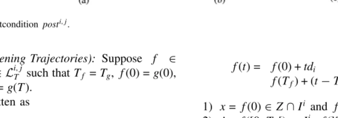
Proposition 1 (Straightening Trajectories): Suppose f ∈ STi,j. Then there existsg∈L
i,j
T such thatTf =Tg,f(0) =g(0), f(Tf) =g(Tf) andf(T) =g(T).
Hence, (17) can be rewritten as
posti,j(Z) =*f(T)| T ≥0, f ∈Li,jT, f(0)∈Z+. (19) Proof:Asf ∈STi,jis a trajectory, for allt∈]0, T[,f˙(t)∈ D(f(t)) and then for all t ∈]0, T[, D(f(t)) == ∅. Therefore f(t)∈Ii∧ ˙f(t)∈Di ift∈]0, Tf[, andf(t)∈Ij∧ ˙f(t)∈Dj
if t ∈]Tf, T[. Asf˙ is piecewise continuous, it is summable
and its sum can be approached by a Riemann sum f(Tf)− f(0) =-Tf 0 f˙(t)dt= TflimP→∞.Pk=0−1P1 f˙ /k+1/2 P Tf 0 . As for any 1 ≤ k < P, f˙(k+1/2P Tf) ∈ Di, the sum belongs to Di,
because Di is convex. As it is also closed, the limit is also
a vector belonging to Di. So there exists di ∈ Di such that -Tf
0 f˙(t)dt= Tfdi. For the same reason, there existsdj ∈ Dj
such that -T
Tff˙(t)dt = (T −Tf)dj. It is now easy to build a
functiongsatisfying the proposition.
We can now give a formulation of posti,j with the time elapse operator [25] in the case whereIi and Ij are convex
polyhedra.
Theorem 1: Let Z ?Di
be the set {z+dt | z ∈ Z, d ∈ Di, t≥0}. Thenposti,j(Z) =
1 / first segment extended to +∞ ! "# $ 2 ( Z∩I¯i)?Di 3 ∩ intersection with frontier and invariants
! "# $ 2¯
Ii∩Fi,j
∩I¯j3 0
# $! "
end of first segment = start of second segment
?Dj 4
∩I¯j∩Xj.
(20) If the sets Z, Di and Dj are convex polyhedra (rather than
general convex sets), all the operations are implemented with-out approximation by standard convex polyhedra operations, as described in [25]. Fig. 8 gives examples. Notice the influence of the configuration at the frontier on the result [Fig. 8(b) and (c)].
Proof: LetGi,j= ¯Ii∩Fi,j
∩I¯j.
(⊆) Suppose y∈posti,j(Z) as defined by (19). Then there
existsx∈Z,T ≥0,f ∈Li,jT withf(0) =x,f([0, Tf[)∈Ii⊆ Xi,f˙([0, Tf[) =di ∈Di, f(]Tf, T])⊆Ij ⊆Xj,f˙(]Tf, T]) = dj ∈Dj. We have f(t) = f(0) +tdi fort∈[0, Tf] f(Tf) + (t−Tf)dj fort∈[Tf, T]. 1) x=f(0)∈Z∩Ii andf(Tf)∈(Z∩Ii)?Di. 2) As f([0, Tf[)∈Ii,f(]Tf, T])⊆Ij, and f is continu-ous, f(Tf)∈I¯i∩I¯j. 3) By definition 1, f(Tf) ∈ Xi∪Xj; if f(Tf) ∈ Xi, as f(]Tf, T])⊆Xj, by continuityf(Tf)∈X¯j; conversely
if f(Tf)∈Xj thenf(Tf)∈ X¯i; thusf(Tf)∈ Fi,j and
together with 2 f(Tf)∈Gi,j.
4) By 1 and 3,f(Tf)∈,= [(Z∩Ii)?Di]∩Gi,j.
5) f(T) =f(Tf) + (T−Tf)dj ∈,?D j
, and by hypothesis
f(T)∈Ij. Thusy∈(,?Dj)∩Ij.
(⊇) Lety∈posti,j(Z) as defined by (20). Then there exists x∈Z∩Ii,t
i, tj ≥0,di∈Di,dj∈Dj such that ,
x+tidi∈Gi,j
y=x+tidi+tjdj∈Ij .
Let us define the function
f(t) = x+tdi for t∈[0, ti] f(ti) + (t−ti)dj for t∈]ti, ti+tj].
We have to show that f ∈ Li,jti+tj and thatf˙(t)∈ D(f)(t) for t∈[0, ti+tj]:
1) f˙([0, ti[) =di∈Di andf˙(]ti, ti+tj]) =di∈Di;
2) f(0)∈Ii,f(ti)∈Gi,j⊆I¯i; as ¯Ii is convex,f([0, ti])∈
¯
Ii; similarly, f([ti, ti+tj]) ∈ I¯j. To conclude we have
to check that f([0, ti[)⊆Ii ⊆Xi andf(]ti, ti+tj])⊆ Ij⊆Xj.
We first show that f([0, ti[) ⊆Ii. If f(ti) ∈ Ii, we have by
convexity f([0, ti[)⊆f([0, ti])⊆Ii. Otherwise, assume that f(ti)∈I¯i\Ii. We prove that ∃t∈]0, ti[:f(t
0)=∈Ii leads to a
contradiction. Lett0 be such at. As Ii is a convex polyhedra
and f(t0) ∈ I¯i\Ii, this means that there exists a constraint a·x+b<0 satisfied byIibut not by ¯Ii, such thata·f(t
0) +b= 0.
Asf(0) ∈ Ii,a·f(0) +b <0. But this implies that for any t > t0,a·f(t) +b >0, so that in particularf(ti)=∈I¯i, which
violates the hypothesis. Thusf([0, ti[)⊆Ii.
The proof off(]ti, ti+tj])⊆Ij is similar.
2) Approximating the Postcondition in the General Case:
If we remove the assumption thatD is constant on each
par-tition member, it is hopeless to give an exactand computable formulation ofposti,j. This indeed reduces to the computation
of post in a non-partitioned system, which has been shown
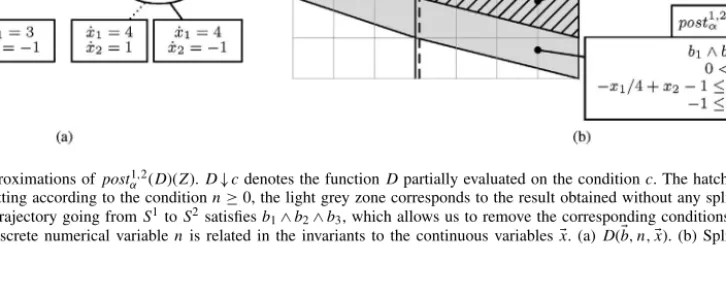
Fig. 9. Different approximations ofpost1,2
α (D)(Z).D↓cdenotes the functionDpartially evaluated on the conditionc. The hatched zones correspond to the
result obtained by splitting according to the conditionn≥0, the light grey zone corresponds to the result obtained without any splitting. Both techniques take into account that any trajectory going fromS1toS2satisfiesb1∧b2∧b3, which allows us to remove the corresponding conditions in the functionD(Ab, n,Ax). Notice also that the discrete numerical variablenis related in the invariants to the continuous variablesAx. (a)D(Ab, n,Ax). (b) Splitting or not w.r.t.n≥0 in postcondition.
consider two solutions.
1) Refine the partition and go back to the situation of the previous section.
2) Replace the function D : S → 2X by a suitable
overapproximation.
For the first case, remark that D is expressed by a
condi-tional function (see Fig. 4) and then, such a finite partition exists. Nevertheless, this solution may require a very detailed partition, which induces an expensive analysis. The second solution we will describe is more flexible and more general; if the partition is not detailed enough, it induces approximations, however those can be controlled and improved by refining the partition.
Let Convex(X) denote the smallest convex set containing X, and
Supp(D) = {x | D(x)==∅} D(X) = {D(x)| x∈X}.
We suggest the following approximation; we define an opera-torposti,j
α obtained by applying (20) with, for k∈ {i, j}: Ik = Convex(Supp(D)∩Xk)
Dk = Convex(D(Xk)).
If D is constant and has a convex support on each partition
member, we fall back to the previous case posti,j α = post
i,j.
Thus, the approximations in postαi,j will be controlled by the
fineness of the partition and will be improved during the partition refinement process. Algorithmically, if D is defined
by a conditional functions (Fig. 4), we just have to compute the convex hull of a finite set of convex polyhedra.
B. Integrating the Discrete State-Space
Now we consider the general case whereS=Q×X. We fix
a partitionS=)kSk of S into abstract values, i.e., such that
for anyk,Sk=γ(Ak) is the conjunction of a Boolean formula
and a convex polyhedra. For the sake of simplicity, we assume that there is no real variable inQ, so that an abstract valueZ
can be decomposed asZ=%ZQ, ZX& ∈A.
1) Exact Postcondition in a Particular Case: We assume here a hypothesis similar to (18)
D(q, x) = ,
Di if (q, x)∈Ii
∅ if (q, x)∈(Si\Ii) (21)
with Ii ⊆ Si an abstract value and Di a convex polyhedra.
We adapt (20) by taking into account the fact that the discrete state-space does not evolve when the time elapses, that is, a trajectory which belong to Si∪Sj is necessarily included in
(SQi ∩SjQ)×(SiX∪SXj). We obtain posti,j(Z) = 5 ZQ ∩IQi ∩IQj 6/2 (ZX∩IXi)?D i3 ∩2Ii X∩Fi,j∩I j X 30 ?Dj7 ∩IXj 8 . (22) 2) Approximating the Postcondition in the General Case:
IfDis not constant on each partition member, we approximate
it as for the purely numeric case. We again take into account the fact that the discrete state-space does not evolve when the time elapses, but in a more subtle way. We define an operator
posti,j
α obtained by applying (22) with IQi = 2Supp(D)∩Si3Q
IXi = Convex'2Supp(D)∩Si∩(IQj ×X)3X( Di = Convex'D'Si∩(IQj ×X)((
and conversely for Dj, Ij Q, andI
j
X. The resulting operator is
denoted by posti,j
TABLE I
Disk Controller’s Analysis (See Fig. 2) Withm=M= 2and!= 0.8 Statistics About the Example
State Variables Input Variables Num. Constraints Cond. Derivative Function 9 bool + 3 num 5 bool + 1 num 16 7 diff. inclusions, guarded by 66 minterms [0,IM] [Om,OM] Options Success ? Partition Size Comments
loc/trans
1 [0,0] [0,0] No refinement No 7/13 Ideal instantaneous reaction 2 [0,0] [0,0] Guided ref. w.r.t.oplus, ominus, mode No 20/70
3 [0,0] [0,0] As 2 + automatic ref. Yes 57/149 Ref. w.r.t.s≥8 ands≤12 (mainly) 4 [0,0] [0.6,0.7] As 3 Yes 58/233
5 [0,0.59] [0.6,0.7] As 3 Yes 86/304
6 [0,0] [0.9,0.9] As 3 No 21/42 Partition simplified at the end
7 [0,0] [k, k] As 3 (Yes) 24/52 k <0.8 inferred necessary condition 8 [0,0] [0.0,0.0] Only automatic ref. Yes 40/119 To be compared to 3
9 [0,0.59] [0.6,0.7] Only automatic ref. Yes 235/850 To be compared to 4 light grey region, withi=1,j=2, and
I1=%b1∧b2∧b3, x1≤0& D1={ ˙x1=3∧ −1≤ ˙x2≤1} I2=%b1∧b2∧b3, x1>0& D2={ ˙x1=4∧ −1≤ ˙x2≤1}.
3) Opening Tests on Discrete Conditions: On the discrete state-space we can also reason by cases, by splitting the argument Z according to discrete conditions which do not
depend on variables involved in continuous evolution. If such a condition c appears in the conditional function D, we
decompose the postcondition as follows:
postαi,j'ite(c, D+, D−)((Z) =
postαi,j(D+)'Z∩!c"( 1 postαi,j(D−)'Z∩!¬c"(
where !c" is the set of states satisfying c. This operator is
more precise, as illustrated in Fig. 9 by the hatched region; here we split the argumentZand the functionDaccording to
the constraintn≥0, which results in
(I1)+= (I1)−=I1 (I2)+= (I2)−=I2
(D1)+={ ˙x1=3∧ ˙x2=−1} (D2)+={ ˙x1=4∧ ˙x2=−1}
(D1)− ={ ˙x1=3∧ ˙x2=1} (D2)−={ ˙x1=4∧ ˙x2=1}.
We can control the tradeoff between precision and efficiency by the depth of such decomposition. Moreover, if now the partition memberS2is refined according to the constraintx2≥
0 intoS+2 and S2−, splitting the argument Z according to the
constraintn≥0 allows us to discover thatn≥0 is a necessary
condition to reachS−2 fromZ, and to use this information for
a further partition refinement.
VI. Experiments A. Implementation
The technique presented in Section V for computing contin-uous postconditions (and preconditions) has been implemented in the NBac tool [29]. NBac implements the principles of
dynamic partitioning and is connected to an input automaton language (implementing the SHA model) and to theLustre
compiler. It exploits the CUDD BDD library [36] and the
APRON numerical abstract domain library [31].NBacworks as follows.
1) It takes a system together with the property to prove, and builds the BDDs and multi-terminal BDDS (MTBDDs)
corresponding to the transition functions and the con-ditional derivative functions.
2) It then perform reachability analysis (from initial states) and coreachability analysis (from final or bad states) on theBoolean abstractionof the system. This corresponds to standard model-checking, with the difference that the numerical constraints appearing in Boolean transition functions are treated as additional Boolean inputs, taking into account some (easy) implication between them. This process can typically infer that transition functions of the form b1’ = (x + 2y > 1); b2’ = (x + 2y > 0)implies that
b,1⇒b,2.
BDDs and MTBDDs are then partially evaluated on
the resulting restricted state-space using a generalized cofactor operator [13].
3) For some properties, step 2 is powerful enough to prove the property. Otherwise, the tool starts a full analysis on both Boolean and numerical variables. It begins with a rough initial partition and alternates analysis and automatic partition refinement steps until proving the property, as described in Section IV.
Compared to the purely discrete version ofNBac, we made two adaptations to the refinement process; first, we took into account the results of continuous postcondition operations when gathering the necessary conditions to jump from one partition member to another one (see Section IV). We also prevented the splitting of a partition member satisfyingx≥0
according to the constraint x ≤ 0. This situation happened
very easily with an automaton like the scheduler depicted in Fig. 2(c), and leads to useless refinements; the case x = 0
should usually remain merged with either the case x <0 or
the case x >0 in the partition (it remains separated when
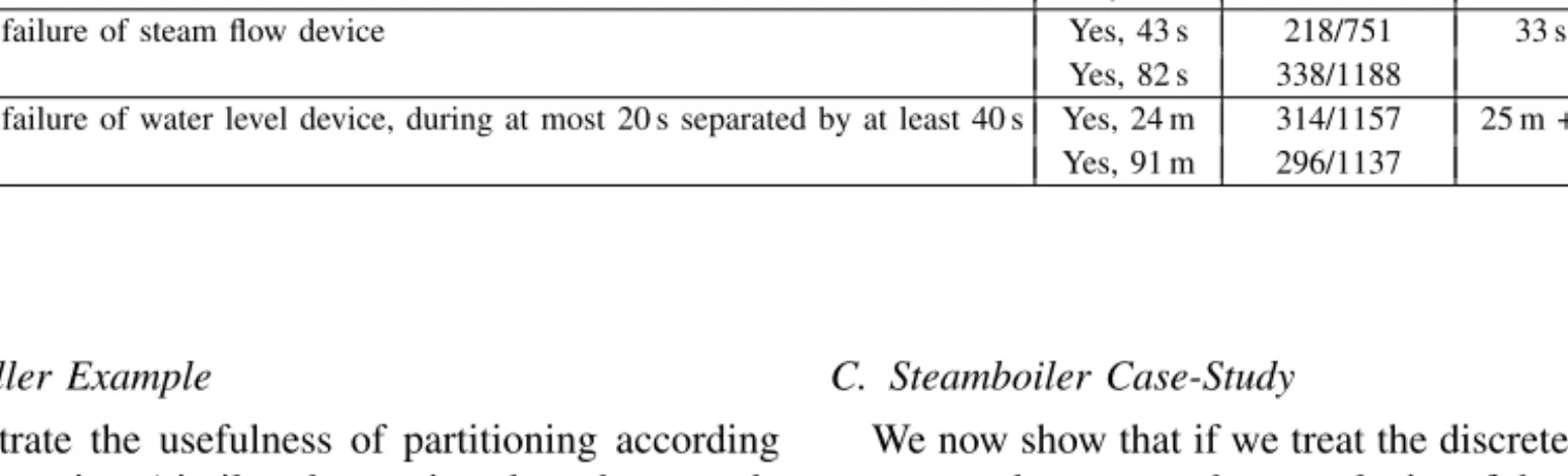
TABLE II
Analysis of the Steamboiler Case Study of [1]. Depending on the Assumption on the Environment, Many Boolean Variables Remain Constant. TheLUSTRECode Has About 500 LOC, and Makes a Large Use ofLUSTREArrays
Statistics About the Example
Assumpt State Variables Input Variables ConstraintsNumerical Cond. Derivative Function 1, 2, 3 85 bool + 8 num 10 bool + 2 num 27 9 inclusions guarded by 268 minterms 3 87 bool + 9 num 11 bool + 2 num 30 17 inclusions guarded by 162 minterms
Assumptions Success Max Alternative
Partition Size (Time, Max. Partition Size)
1min No failure Yes, 44 s 218/751 33 s + 105 s, 1212/3809
1max – Yes, 81 s 338/1188
2min Possible failure of pump 0 Yes, 235 s 879/3297 3 m + 14 m, 4964/20 122
2max – Yes, 138 s 557/2083
3min Possible failure of steam flow device Yes, 43 s 218/751 33 s + 105 s, 1212/3809
3max – Yes, 82 s 338/1188
4 min Possible failure of water level device, during at most 20 s separated by at least 40 s Yes, 24 m 314/1157 25 m + >60 m, >6201/28 209
4max – Yes, 91 m 296/1137
B. Disk Controller Example
We first illustrate the usefulness of partitioning according to numerical constraints (similar observations have been made in the context of predicate abstraction [3]). We analyzed the system described in Section II and Fig. 2.
We verify that the disk motor speed never stays more than 8 consecutive time units outside the desired range. Thus, we already need to partition the state-space according to a numerical constraint (d ≥8) in order to separate “good” and
bad sets of states.
We start all analyses with the control structures of the scheduler and the property observer process made explicit in the partitioned abstract domain. Table I gives some statistics about the example, and details our experimental results for various parameters and options. Concerning the statistics about the derivative function, notice that the number of distinct differential inclusions does not correspond to the number of modes in classical model. For instance, if one considers the conditional derivative function of the scheduler of Fig. 2(c), it contains only two inclusions∅and˙t= 1, but this corresponds
to four modes. A timed automaton [4] generates in our model a derivative function with only two inclusions:∅(when outside the global invariant), and the set9ic˙i= 1 which specifies that
all clocks have a rate of 1.
In Table I, lines 1–3 show that we need to refine the partition w.r.t. numerical constraints in order to prove the property. In particular, line 3 shows that we need to partition according to s ≥ 8 and s ≤ 12 to make the invariants of Fig. 2(d)
convex. Lines 3–5 illustrate that more nondeterminism in the scheduler requires more partition refinement steps. We fail to show the property ifOm=OM =0.9 (line 6). We then find a
necessary condition,k <0.8, on the parameterk=Om=OM
(line 7) for the property to hold. Thus, we are able to analyze the influence of the reaction delay between input and output of the discrete controller. Lines 8–9 show the analysis without initial guided refinement; the results are comparable (line 8) or worse (line 9).
C. Steamboiler Case-Study
We now show that if we treat the discrete part symbolically, we can scale up w.r.t. the complexity of the discrete controller. The case-study is the steam-boiler controller of Abrial [1]. We implemented faithfully the original specification of [1] in Lustre (with three instead of four pumps and without initialization phase). Hybrid automata model the behavior of physical quantities and the scheduler depicted in Fig. 2(c) (with IM =Om=OM =0 as in [1]). The controller can enable or disable 0, 1, 2, or 3 pumps at each step, and takes into account detected failures. It needs some kind of anticipation, as there is a delay when switching up a pump. Moreover, the controller has to maintain its own view of the environment, and to exploit this simulated view in order to take adequate decision, for instance in case of water-level device failure. The first versions of the controller were wrong and required some refinements to be correct (limit cases were detected using a Lustre simulator and a discrete version of the environment).
The property to be verified is that the water levelqstays in
[M1, M2]. This property is decomposed into two properties
(minimal and maximal bound). We check it for various as-sumptions on the environment, modeling different fault mod-els. Indeed, if all the devices silently fail, the property on the water level cannot be ensured by the controller. We considered thus four fault models on the environment. The top table of Table II gives statistics about the global model obtained, in terms of number of variables, numerical constraints, and derivative functions. It should be noted that depending on the considered fault model, several Boolean variables may be constant, so we give below other means if evaluating the complexity of the global model.
Table II presents our experimental results. “Max partition size” refers to the maximal size of the partition in the course of the refinement process. We used the control structure of the hybrid part of the system as the initial partition, and we then relied on the automatic refinement heuristics described
in [29] [except for assumption 4, where we guided the first refinement step according to the state of the pumps (on or off)]. Assumption 4 corresponds to the most complex fault model: the controller has to use its own simulation of the water level to take decisions, and the property is true only if the failure does not last too much, and if there is enough time between two failures to allow the system to go back to a “normal” state. For this assumption, the number of refinement steps is comparable to the other experiments, but the analysis time is much higher. This is essentially due to more complex BDDs and convex polyhedra
compu-tations.
As the other verification tools for hybrid systems accept only lower-level non-symbolic automata, which manipulates only numerical variables, making a direct comparison would have required non-trivial translators and would have been very involving. We make here a comparison with the following alternative analysis method, consisting of:
1) performing a reachability analysis of the Boolean ab-straction of the system, and restricting the initial parti-tion to the computed state-space;
2) refining incrementally the partition according to all
Booleans;
3) and last analyzing and further refining the partition until success.
The column “Alternative” gives the time and max. partition size obtained by this method. The time is decomposed in the time of steps 1 + 2 and the time of step 3. The max. partition size first gives an idea of the size of the reachable part of a non-symbolic automaton model, and also shows that our automatic refinement is quite good, as our method succeeds to prove the property on a much smaller partition. Regarding time, the alternative technique is always more expensive (by factors of 3–4), or even fails for assumption 4.
Regarding the level of automation, the initial partition we provide is reasonable; it is the explicit control structure of the hybrid environment. The very first refinement steps are guided and further partition according to the state of the three pumps. Then we rely only on automatic refinement heuristics described in [29]. For assumption 4, we added a few more guided refinement steps, by considering some state variables of theLustrecontroller that corresponds to state variables of the environment.
More details can be found at http://pop-art.inrialpes.fr/people/ bjeannet/nbachybrid/nbachybrid.html.
VII. Conclusion
We first proposed a symbolic model for hybrid systems, SHA, that allowed us to embed directly higher-level Lus-tre program in a hybrid automaton and also to implement an analysis technique which can combine symbolically both the discrete and the continuous behavior. We then defined the abstract postcondition induced by this symbolic setting, in the context of a partitioned domain.
We implemented the proposed method and we succeeded to prove the global safety property of a very faithful implemen-tation of the steamboiler case study, for various assumptions
on the environment and possible failures (occurrences and/or duration). The alternative technique that enumerates all reach-able Boolean valuations before analyzing numerical varireach-ables proved to be much slower, or impractical in complex cases.
We insist on the fact that previous attempts to verify hybrid models of this case study focused on the physical model of the devices and considered a very simplified version of the software controller. Besides the limitations of the used verification methods, they could hardly specify a detailed model without relying on a real programming language like
Lustre.
Our experiments also raised some issues. First, we made the classical observation that guiding the refinement process by providing some (obvious) control structure [like the scheduler of Fig. 2(c)] helps a lot. Related to this is that the refinement process performs only partition refinement, and does not have criteria to group back partition members when it seems that the refinement did not really improve the precision. It also appears that the widening in some cases loses important information, which causes further refinement steps. The guided widening technique of [20] improves the precision, but makes the analy-sis much more expensive. Another point is that it is difficult to manually inspect on the examples how the refinement proceeds w.r.t. the originalLustre program, because our tool exploits a lower-level representation of theLustreprogram that loses its structure. As a consequence, we plan to connect our tool directly to the Lustre language in order to implement more sophisticated refinement techniques, to identify more easily performance bottlenecks, and to experiment a larger set of examples.
It would be also very interesting to adapt and experiment the
k-induction approach (see [22]) in the case of hybrid systems,
and to compare it to this approach. The two approaches are indeed quite complementary; the k-induction approach
ignores reachability information and performs only bounded propagation of properties, but in aexact way; our abstract in-terpretation based approach performs unbounded propagation at the cost of approximations.
Acknowledgment
The authors thank the anonymous reviewers for their com-ments and suggestions which were very helpful to improve this paper.
References
[1] J.-R. Abrial, E. B¨orger, and H. Langmaack, Eds.,Formal Methods for Industrial Applications: Specifying and Progr. the Steam Boiler(Lecture Notes in Computer Sciences, vol. 1165). Berlin, Germany: Springer, 1996.
[2] R. Alur, C. Courcoubetis, N. Halbwachs, T. Henzinger, P. Ho, X. Nicollin, A. Olivero, J. Sifakis, and S. Yovine, “The algorithmic analysis of hybrid systems,”Theor. Comput. Sci. B, vol. 138, no. 1, pp. 3–34, Feb. 1995.
[3] R. Alur, T. Dang, and F. Ivancic, “Counter-example guided predicate abstraction of hybrid systems,” inProc. TACAS, LNCS 2619. 2003, pp. 208–223.
[4] R. Alur and D. L. Dill, “A theory of timed automata,”Theor. Comput. Sci., vol. 126, no. 2, pp. 183–235, Apr. 1994.