QUANTITATIVE FINANCE
RESEARCH CENTRE
�������������������� ���������������
Q
UANTITATIVEF
INANCER
ESEARCHC
ENTREResearch Paper 242 January 2009
Alternative Defaultable Term Structure Models
Nicola Bruti-Liberati, Christina Nikitopoulos-Sklibosios, Eckhard Platen and Erik Schlögl
Alternative Defaultable Term Structure Models
Nicola Bruti-Liberati†1, Christina Nikitopoulos-Sklibosios2,
Eckhard Platen3 and Erik Schl¨ogl2
January 16, 2009
Abstract. The objective of this paper is to consider defaultable
term structure models in a general setting beyond standard risk-neutral models. Using as numeraire the growth optimal portfolio, defaultable interest rate derivatives are priced under the real-world probability measure. Therefore, the existence of an equivalent risk-neutral probability measure is not required. In particular, the real-world dynamics of the instantaneous defaultable forward rates under a jump-diffusion extension of a HJM type framework are derived. Thus, by establishing a modelling framework fully under the real-world probability measure, the challenge of recon-ciling real-world and risk-neutral probabilities of default is deliber-ately avoided, which provides significant extra modelling freedom. In addition, for certain volatility specifications, finite dimensional Markovian defaultable term structure models are derived. The paper also demonstrates an alternative defaultable term structure model. It provides tractable expressions for the prices of default-able derivatives under the assumption of independence between the discounted growth optimal portfolio and the default-adjusted short rate. These expressions are then used in a more general model as control variates for Monte Carlo simulations of credit derivatives.
Mathematics Subject Classification: primary 60H10; secondary 65C05.
JEL Classification: G10, G13
Key words and phrases: defaultable forward rates, jump-diffusion processes, growth optimal portfolio, real-world pricing.
1
Introduction
This paper considers defaultable term structure models under the real-world prob-ability measure. When modelling credit risk, the choice of an appropriate equiva-lent risk-neutral pricing measure has never been a straightforward task. Realistic
1In memory of our beloved colleague and friend.
2University of Technology Sydney, School of Finance & Economics
3University of Technology Sydney, School of Finance & Economics and Department of Mathematical Sciences
market models, see Heath and Platen (2002a) and Platen (2002), may not even admit an equivalent risk-neutral probability measure. We argue in this paper that the real-world pricing approach provides a significant advantage over the tra-ditional risk-neutral pricing framework and generalises the existing risk-neutral approach for pricing derivatives subject to default.
In a market driven by continuous and discrete trading uncertainty, we develop jump-diffusion interest rate term structure models by extending the classical Heath, Jarrow, and Morton (1992) (HJM) framework. As a natural application of jump-diffusion models, credit events including defaults are modelled as jumps. The paper derives the real-world HJM type dynamics of the instantaneous de-faultable forward rates. The novelty of this result is that we obtain analogous dynamics of the defaultable forward rates, as for instance derived by Sch¨onbucher (1998), yet they are described under the real-world probability measure and avoid the restrictive assumption on the existence of an equivalent risk-neutral proba-bility measure. Since we do not rely on a change of the probaproba-bility measure, the jump intensities we deal with are real-world intensities.
The proposed approach yields a consistent framework that has the power to connect real-world default probabilities and observed credit spreads under the real-world probability measure. This unifies the pricing and hedging of derivative instruments, traditionally performed under some putative risk-neutral probability measure, with the tasks of risk measurement such as VaR and portfolio optimiza-tion. The latter require in any case the use of the real-world probability measure. One can say that risk-neutral pricing is a kind of relative pricing. As soon as some market participant places some derivative price in the market, others can use it to calibrate their risk-neutral model and form consistent prices for fur-ther derivatives. This does not prevent a development where over long periods of time such prices can be way out from what may be realistically sustainable, as observed prior to the recent subprime crisis. Real-world pricing however, is a form of absolute pricing. Taking historical data and economic arguments into account one does not rely on the presence of some credit derivatives in the mar-ket for calibrating the model. This could have potentially avoided the situation where an entire industry failed to value correctly the risk in subprime credit derivatives. Real-world pricing is nothing but an investment decision where the investor values a claim with respect to his or her best performing portfolio, the growth optimal portfolio (GOP), without the potential distortions by using an artificial risk-neutral measure.
The fundamental principle of real-world pricing is that by taking as numeraire the GOP, pricing can be performed under the real-world or historical probability measure, see Platen and Heath (2006). More specifically, the value of a derivative is expressed in terms of a real-world conditional expectation. This provides the considerable advantage that the existence of an equivalent risk-neutral probability measure is not required. Consequently, a richer modelling world results than is available under the classical risk-neutral approach. As shown in Platen and
Heath (2006), a diversified world stock index can be used as a proxy of the GOP. A particular form for the stochastic differential equation (SDE) of the GOP for a market driven by jump diffusions emerges. The generalised volatilities and the jump coefficients of the GOP characterize the market prices of diffusion and jump risk, respectively. The dynamics of the GOP are determined by these market prices of risk, as well as the risk-free short rate. In the literature, the market price of jump risk is usually assumed to be zero. The proposed approach allows to relax this assumption.
A class of alternative defaultable term structure models, which do not admit an equivalent risk-neutral probability measure, will be demonstrated. These gen-eral jump- diffusion models do not normally have closed form solutions, therefore Monte-Carlo simulation is the typical numerical approach to handle these mod-els. However, standard Monte-Carlo simulation by using an Euler scheme or similar standard schemes may not be adequate. The proposed model requires the simulation of strictly positive affine processes. This type of processes typ-ically encounters simulation problems when the process comes near zero under standard simulation schemes. This can be resolved by using an exact simulation scheme, see for instance Broadie and Kaya (2006). Furthermore, the efficiency of the Monte-Carlo simulation can be significantly improved by using variance re-duction methods, see Kloeden and Platen (1999) and Heath and Platen (2002b). In this paper, we demonstrate how a class of tractable defaultable term structure models can be obtained. More specifically, by assuming independence between the discounted GOP and the default-adjusted short rate, we first obtain closed form expressions for the prices of defaultable bonds and potentially other derivatives. Then in the more general case, we use an exact simulation scheme, in the spirit of Platen and Rendek (2009), which guarantees strict positive paths. However, like with any raw Monte-Carlo simulations, it can become computationally expensive and therefore, a variance reduction technique is highly recommended. In fact, the above explicit formulae for the defaultable bonds can be used as control variates or in other variance reduction methods for Monte Carlo simulations of the more general defaultable term structure models.
The paper is structured as follows. Section 2 provides the theoretical background for the modelling and pricing of real-world defaultable term structure models. In addition, we derive for certain volatility and intensity specifications tractable finite dimensional Markovian defaultable term structures. Section 3 introduces an alternative defaultable term structure model, with analytic expressions for prices of defaultable bonds. In Section 4, these analytic expressions for defaultable bond prices serve as control variates for an illustrative example on the effect of a variance reduction method in Monte Carlo simulations for pricing under a more general model. Section 5 concludes.
2
Real-World Pricing for a Defaultable Term
Structure of Interest Rates
2.1
Modelling Traded Uncertainty
On a filtered probability space (Ω,AT¯,A, P), ¯T ∈ (0,∞) with A = (At)t∈[0,T¯],
satisfying the usual conditions, we model the continuous traded uncertainty as an A-adapted, m−dimensional Wiener process W ={Wt = (Wt1, . . . , Wtm)⊤, t ∈
[0,T¯]}. The event driven traded uncertainty is modelled by a Poisson random measure p, which is defined below. Given a mark space (E,B(E)), with E ⊆
R\{0}, we define on E ×[0,T¯] an A-adapted Poisson random measure p(dv, dt)
characterised by a time-varying intensity measure φ(dv, t)dt. We assume almost surely finite total intensity λt = φ(E, t) < ∞, t ∈ [0,∞). Note that we allow
the intensity measureφ(dv, t)dt, and thus the total intensityλt, to be stochastic.
Herep={pt:=p(E ×[0, t]), t ∈[0,T¯]}represents a stochastic process that counts
the total number of jumps, that is modelled events occurring in the time inter-val [0, t]. The Poisson random measure p(dv, dt) generates a sequence of pairs
{(τi, υi), i ∈ {1,2, . . . , pT¯} }, where {τi : Ω → R+, i ∈ {1,2, . . . , pT¯} } is the
se-quence of jump times of the Poisson processpand{υi : Ω→ E, i∈ {1,2, . . . , pT¯} }
is the corresponding sequence of independent, identically distributed marks υi
with probability density φ(dv,tλt ). One can interpret τi as the time of the ith event
and the mark υi as its magnitude. By compensating the Poisson measure we
obtain the jump martingale measure q(dv, dt) =p(dv, dt)−φ(dv, t)dt.
Additionally, we will assume that the drift, diffusion and jump coefficients of the factor processes driving the market dynamics to be predictable and regular enough such that the corresponding system of SDEs admits a unique strong solution and the manipulations we perform are possible. It will be not necessary to describe the primary securities of the market in detail. What is essentially needed for term structure modelling is the characterization of the GOP and the savings account.
2.2
Growth Optimal Portfolio with Default
The GOP is defined as the portfolio which maximises the expected logarithm of terminal wealth for all times t ∈ [0,T¯], see Kelly (1956), Karatzas and Shreve (1998) and Platen (2002). In our continuous time setting, the existence of a GOP implies no arbitrage in the strong sense of Platen (2002). Christensen and Platen (2005) consider a general jump-diffusion setting with stochastic jump sizes and obtain a generalised GOP, which we use here as our basis.
We denote the market prices of Wiener process risk by the predictable vector process Θ = {θt = (θ1t, θt2, . . . , θmt )⊤, t ∈ [0,T¯]}, and the density of the market
price of jump risk by the predictable and bounded process ψ(v) = {ψ(v, t), t ∈
predictable default-free short rate process r = {rt, t ∈ [0,T¯]}. Then the unique
generalised GOP, Sδ∗
t , satisfies the SDE
dSδ∗ t =Stδ−∗ rtdt+ m X i=1 θti(θitdt+dWti) (2.1) + Z E ψ(v, t) 1−ψ(v, t)(ψ(v, t)φ(dv, t)dt+q(dv, dt)) ,
for all t ∈[0,T¯], withSδ∗
0 = 1, see Christensen and Platen (2005). Note that the
dynamics of the GOP are determined solely by the default-free short rate rt, the
vector of market prices of Wiener process risk θt and the density of the market
price of jump risk ψ(v, t). Moreover, the total risk premium of the GOP at time
t ∈[0, T] is given by ϑSt =θ⊤t θt+ Z E (ψ(v, t))2 1−ψ(v, t)φ(dv, t). (2.2)
From the SDE (2.1) we obtain that at the ith jump time τ
i of the Poisson jump
measure we have Sδ∗ τi −S δ∗ τi− =S δ∗ τi− ψ(υi, τi−) 1−ψ(υi, τi−) . (2.3)
If we assume that the GOP is observable, then the density of the market price of jump risk can be observed in terms of the GOP values before and after jump times as ψ(υi, τi−) = 1− Sδ∗ τi− Sδ∗ τi . (2.4)
This gives access to the estimation and calibration of the function ψ(·,·), which is crucial for realistic modelling. Note also that the volatility of the GOP, |θt|=
pPm
i=1(θti)2 is observable. However, the drift of a process is usually very difficult
to estimate. Fortunately, such estimation is not necessary here since in (2.1), the drift depends on the observable short rate, GOP volatility, market price of jump risk density and jump intensity.
2.3
Real-World Pricing
In the following we will choose the GOP as numeraire or benchmark and will use the wordingbenchmarked when a price or value is expressed in units of the GOP. It has been shown in Platen and Heath (2006) that any nonnegative portfolio when expressed in units of the GOP forms an (A, P)-supermartingale, and in the set of all supermartingale price processes that match a given future payoff, the martingale is the one with the minimal value. Furthermore, we call a price
process fair when it forms a martingale when benchmarked. Therefore, by re-questing benchmarked derivative prices to be fair, the pricing of derivatives is performed under the real-world probability measure with the GOP as numeraire. Due to the supermartingale property of all benchmarked nonnegative portfolios, fair portfolios are minimal among those that replicate the same payoff. This yields the following concept of real-world pricing, see Long (1990) and Platen and Heath (2006).
Definition 2.1 For T ∈ [0,T¯] assume that HT is an AT-measurable contingent
claim delivered at maturity T, which satisfies
E HT Sδ∗ T <∞ almost surely. (2.5)
Then the fair price process VHT = {VHT(t), t ∈ [0, T]} of HT is given by the real-world pricing formula
VHT(t) =S δ∗ t E HT Sδ∗ T |At , (2.6) for all t ∈[0, T].
Real-world pricing is performed by using in the evaluation the real-world expec-tation. Therefore, no change of probability measure is required. If an equivalent risk-neutral probability measure exists in a complete market, then the real-world pricing formula (2.6) can be shown to coincide with the risk-neutral one, see Platen and Heath (2006). Real-world pricing generalizes risk-neutral pricing and can be applied also under models which do not admit an equivalent risk-neutral probability measure, as will be demonstrated in Section 3.
2.3.1 Real-World Defaultable Zero-Coupon Bond Dynamics
LetPd(t, T) be the price at timet ∈[0, T] of a defaultable zero-coupon bond with
maturity T ∈ [0,T¯]. We assume fractional recovery upon default, adapting the setup of Sch¨onbucher (1998). Typically, the fractional recovery arises as a result of restructuring and some reduction of the notional in case of default. Defaults can occur at jump timesτi ≤T. At each default timeτi, the fractional loss quota υi of the bond price is drawn from E=(0,1]. We denote by ¯Qt the reduction on
the bond face value due to defaults until time t. Note that this approach allows for multiple defaults. At maturity T, the defaultable bond processPd(·, T) pays
out ¯ QT := Y i:τi≤T (1−υi), (2.7)
the remaining face value after all fractional losses. The face value ¯Qt is assumed
to be the solution of the SDE
dQ¯t=−Q¯t−
Z 1
0
vp(dv, dt), (2.8)
fort∈[0, T], subject to the initial condition ¯Q0 = 1. By using (2.6) and assuming
E (Sδ∗ T )−1
<∞, the real-world price at time t∈ [0, T] for the defaultable zero-coupon bond with maturity T is
Pd(t, T) =Sδ∗ t E ¯ QT Sδ∗ T |At , (2.9)
for t ∈ [0, T], T ∈ [0,T¯]. Relationship (2.9) guarantees that the benchmarked defaultable zero-coupon bond, denoted as
ˆ Pd(t, T) = P d(t, T) Sδ∗ t , (2.10)
is an (A, P)-martingale and thus, fair. Therefore, it satisfies a driftless SDE of the form dPˆd(t, T) = −Pˆd(t−, T) m X i=1 ˆ σi(t, T)dWi t + Z 1 0 ˆ β(v, t, T)q(dv, dt) ! . (2.11) Here ˆσi(·, T), for i ∈ {1,2, . . . , m}, and ˆβ(v,·, T) are predictable stochastic
pro-cesses modelling the benchmarked defaultable bond volatilities and jump coef-ficient, respectively. By (2.1), (2.10), (2.11) and Itˆo’s formula we obtain the dynamics of the defaultable zero-coupon bond price as
dPd(t, T) =Pd(t−, T) " rt+ m X i=1 σi(t, T)θit+ Z 1 0 β(v, t, T)(ψ(v, t)−1)φ(dv, t) ! dt + m X i=1 σi(t, T)dWti+ Z 1 0 β(v, t, T)p(dv, dt) # , (2.12)
for all t ∈[0, T], with defaultable bond volatilities
σi(t, T) =θti−σˆi(t, T), (2.13)
i∈ {1,2, . . . , m}, and jump coefficient
β(v, t, T) = ψ(v, t)−βˆ(v, t, T)
1−ψ(v, t) . (2.14) Note that at each default time τi, the relative change in the bond price
Pd(τ
i, T)−Pd(τi−, T) Pd(τ
i−, T)
can be decomposed into two distinct effects. First, after default restructuring of the defaulted obligor’s business takes place, and there is a reduction of the claims of the bond holders, which leads to a fractional loss equal to υi in the
bond price. Second, additionally, the market’s valuation of the bond can change, see Sch¨onbucher (1998). One can model both effects by decomposing the jump coefficient of the defaultable bond as
β(v, t, T) = βM(v, t, T)−v, (2.16)
where βM(v, t, T) reflects the jump due to the change in the market valuation.
2.3.2 Real-World Defaultable Forward Rate Dynamics
We define the instantaneous defaultable forward rate fd(t, T) at time t ∈ [0, T],
with T ∈[0,T¯], as
fd(t, T) :=− ∂
∂T ln(P
d(t, T)). (2.17)
We also define the predictable defaultable short rate process as rd = {rd
t :=
fd(t, t), t ∈ [0, T]}. Then by taking into account the face value reduction ¯Q t of
the bond at time t, the value of the defaultable bond Pd(t, T) can be expressed
as Pd(t, T) = exp − Z T t fd(t, s)ds ¯ Qt. (2.18)
Note that by relationships (2.10) and (2.17) the defaultable forward rate can be equivalently expressed in terms of the benchmarked defaultable bond as
fd(t, T) =− ∂
∂T ln( ˆP
d(t, T)). (2.19)
As shown in Appendix A, this yields the following result, where ˆσi(t, T), i ∈ {1,2, . . . , m}, and ˆβ(v, t, T) are defined in (2.11).
Proposition 2.2 The real-world dynamics of the instantaneous defaultable for-ward rate are given by
dfd(t, T) = µd(t, T)dt+ m X i=1 σdi(t, T)dWti+ Z 1 0 βd(v, t, T)p(dv, dt), (2.20) where µd(t, T) = m X i=1 σi d(t, T) Z T t σi d(t, s)ds+θti (2.21) − Z 1 0 βd(v, t, T) exp − Z T t βd(v, t, s)ds (1−ψ(v, t))(1−v)φ(dv, t),
and σdi(t, T) = ∂ ∂Tσˆ i(t, T), (2.22) βd(v, t, T) = ∂ ∂Tβˆ(v, t, T) 1−βˆ(v, t, T). (2.23)
The defaultable forward rate drift restriction (2.21) has a similar structure to the HJM restriction described in Sch¨onbucher (2003), which was derived under some risk-neutral probability measure. However, the drift restriction (2.21) holds under the real-world probability measure under which W1
t, . . . , Wtm are Wiener
processes and p(·,·) is a Poisson measure with intensity measure φ(dv, t). This provides an advantage of the benchmark approach over the risk-neutral approach concerning the estimation of default intensities and probabilities. Real-world default probabilities can be estimated using historical data and credit spreads, or by economic reasoning. In contrast, risk-neutral default probabilities can be obtained only by using some model applied to observed credit spreads. As previ-ously discussed, these spreads can be way out from reality if one relies on relative pricing. By using the real-world probability measure for calibration and pricing, the benchmark approach avoids the challenge of estimating hypothetical risk-neutral probabilities of default from credit derivatives in the market or by other means. Albanese and Chen (2005) provide an interesting study of this controver-sial problem. As we have already pointed out in the introduction, we perform a type of absolute pricing, whereas the standard approach yields relative prices. Note that by (2.14), (2.16) and (2.23), the defaultable forward rate jump coeffi-cient can be expressed as
βd(v, t, T) = ∂
∂TβM(v, t, T) v−1−βM(v, t, T)
. (2.24)
This shows that if in our setting the jumps in the defaultable bond price due to changes in the market valuation at default do not depend on the maturityT of the bond, this means βM(v, t, T) = βM(v, t), then we obtain continuous defaultable
forward rates.
In Appendix B, we derive a relationship for the short rate spread in terms of the real-world intensity measure and the market price of jump risk as
rdt −rt =
Z 1
0
(1−ψ(v, t))vφ(dv, t). (2.25)
If an equivalent risk-neutral probability measure Λ exists, then the risk-neutral intensity measure φΛ(dv, t) can be expressed as φΛ(dv, t) = (1−ψ(v, t))φ(dv, t)
and the spread (2.25) reduces to
rtd−rt=
Z 1
0
which is equivalent to a result in Sch¨onbucher (1998). However, there is no need to restrict our modelling by requiring the existence of an equivalent risk-neutral probability measure.
2.4
Finite Dimensional Markovian Term Structures
When keeping the framework on the current general level, one faces certain math-ematical challenges concerning the consistency of the model in the context of enlargement of filtration, see Elliott, Jeanblanc, and Yor (2000). In practice one needs tractable models that, in principle, lead to Markovian model structures, which usually avoid consistency problems of this kind. Otherwise, the need for the description and storage of the entire history of the market would create un-solvable practical obstacles. However, even in Markovian settings, one has to be parsimonious with the number of factors and parameters in the model in order to keep the dimensionality of the problem manageable and to allow a proper fitting of market data.
Though very flexible, HJM term structure models are, in general, non-Markovian. It has been demonstrated in Chiarella, Schl¨ogl, and Nikitopoulos (2007) that, un-der the existence of an equivalent risk-neutral probability measure, specific for-ward rate volatility structures can produce finite dimensional Markovian default-able HJM models which are computationally tractdefault-able. It will be shown next that certain forward rate volatility specifications will lead to tractable finite dimen-sional Markovian dynamics for the defaultable interest rate term structure under the real-world probability measure without relying on any risk-neutral framework.
Assumption 2.3 For T ∈ (0,T¯] and i ∈ {1, . . . , m}, the diffusion coefficients (2.22) of the defaultable forward rate are of the form
σdi(t, T) = ¯σid(t,Ft) e−
RT t k
i
σ(s)ds, (2.27)
and the jump coefficient (2.23) is of the form
βd(v, t, T) = ¯βd(v, t)e−
RT
t kβ(s)ds, (2.28) where ki
σ(t), kβ(t) are deterministic functions of time, integrable in [0,T]; and
¯
σi
d = {σ¯di(t,Ft), t ∈ [0, T]} and β¯d = {β¯d(v, t),(v, t) ∈ (0,1]×[0, T],}
charac-terise well-defined functions, with Ft= (rdt, fd(t, T1), . . . , fd(t, Tz))⊤, for z ∈N= {1,2,3, . . .} and t < T1 < . . . < Tz. In addition, the density of the market price
of jump risk ψ ={ψ(v, t),(v, t)∈(0,1]×[0, T]} and the jump intensity measure
φ(dv, t), t∈[0, T], are deterministic.
The key property of the proposed volatility structure is the separability of the time dependent component from the maturity dependent component. The resulting Markovian dynamics of the defaultable short rate are derived in Appendix C and are summarized in the following proposition.
Proposition 2.4 Under Assumption 2.3 the real-world dynamics of the default-able short rate are given by
drdt = h ξt+Eβ(t) + m X i=1 Eσi(t)− m X i=2 (kiσ(t)−k1σ(t))D i σ(t)−(kβ(t)−kσ1(t))Dβ(t) + m X i=1 ¯ σdi(t,Ft)θti−kσ1(t)rt i dt+ m X i=1 ¯ σdi(t,Ft)dWti+ Z 1 0 ¯ βd(v, t)p(dv, dt), (2.29)
with the state variables Ei
σ(t), Diσ(t), Dβ(t) defined as Eσi(t) = Z t 0 σdi(u, t) 2 du, (2.30) Dσi(t) = Z t 0 σdi(u, t) Z t u σid(u, s)dsdu+ Z t 0 σdi(u, t)(dWui +θiudu), (2.31) Dβ(t) =− Z t 0 Z 1 0 βd(v, u, t)e− Rt uβd(v,u,s)ds(1−v)(1−ψ(v, u))φ(dv, t)du + Z t 0 Z 1 0 βd(v, u, t)p(dv, du), (2.32)
respectively, and the time varying coefficients Eβ(t) and ξt are determined by Eβ(t) = Z t 0 Z 1 0 βd(v, u, t)2e− Rt uβd(v,u,s)ds(1−v)(1−ψ(v, u))φ(dv, t)du − Z 1 0 ¯ βd(v, t)(1−v)(1−ψ(v, t))φ(dv, t), (2.33) ξt= ∂ ∂Tf d(0, T) |T=t+kσ1(t)fd(0, t), (2.34) respectively.
The stochastic quantities Ei
σ(t), Dσi(t) and Dβ(t) form state variables of linear
mean reverting SDEs, as the following proposition demonstrates.
Proposition 2.5 Under Assumption 2.3, the stochastic quantities Ei
σ(t), Dσi(t)
and Di
β(t) satisfy the SDEs,
dEσi(t) = [(¯σid(t,Ft))2−2κiσ(t)Eσi(t)]dt, dDσi(t) = [Eσi(t)−κiσ(t)Dσi(t)]dt+ ¯σid(t,Ft)(dWti+θtidt), and dDβ(t) = [Eβ(t)−κβ(t)Dβ(t)]dt+ Z 1 0 ¯ βd(v, t)p(dv, dt).
Proof. Taking the differentials of the stochastic quantities (2.30), (2.31) and (2.32), the above equations are obtained. Additionally, to obtain a closed Markovian system, the stochastic market prices of Wiener process riskθi
tshould satisfy an SDE with coefficients depending on the
state variables of that system. Thus, the finite dimensional Markovian system with the state vector (rd
t, fd(t, T1), . . . , fd(t, Tz),θt1, Eσ1(t),Dσ1(t),. . ., θmt , Eσm(t), Dm
σ (t), Dβ(t))⊤, for z, m ∈ N determines the short rate dynamics (2.29). Recall
that the state variables fd(t, T
k), k ∈ (1,2, . . . , z), satisfy the SDE (2.20) under
the volatility structure of Assumption 2.3. Alternatively, the market prices of Wiener process risk can be modelled by an additional set of state variables, as these are the only state variables driving the dynamics of the discounted GOP. Assumption 2.3 imposes the restriction of a deterministic market price of jump risk ψ(v, t) and a deterministic jump intensity φ(dv, t). A general specification which would allow stochastic market price of jump risk and stochastic jump in-tensity is feasible, but would lead to Markovian structures only in the case of constant jump coefficients. For a jump coefficient of the form (2.28) an approxi-mate Markovianisation can be achieved along the lines of Chiarella, Schl¨ogl, and Nikitopoulos (2007).
3
Tractable Defaultable Multi-Factor Models
A class of parsimonious defaultable multi-factor models will be presented next. These models provide computationally tractable formulas for defaultable zero-coupon bonds. The numerical evaluation is conveniently performed in a multi-factor setting of the following kind which represents a special case of the previous class of Markovian models.
3.1
Real-World Default-Adjusted Short Rate
We start from a d-dimensional factor process whose dynamics are described by the SDE
dXt =a(t, Xt)dt+b(t, Xt)dWt, (3.1)
where W denotes the m-dimensional standard Wiener process representing the continuous traded underlying. In this section we assume, for simplicity, that the jump process generating defaults is a compound Cox process, also called compound doubly stochastic Poisson process, see for instance Duffie (2005), with stochastic intensity process λ ={λt, t ∈[0,∞)}. We suppose that the σ-algebra
generated by the factor process X = {Xt, t ∈ [0, T]} defines the filtration G =
(Gt)t∈[0,∞) ⊂(At)t∈[0,∞) =A. Moreover, we suppose that the default-free interest
ratert, the discounted GOP ¯Stδ∗ = Sδ∗
t
S0
be expressed as measurable nonnegative functions of time t and Xt. Therefore,
they are adapted to G = (Gt)t∈[0,∞). The jump sizes υi, which represent the
fractional loss quota, are independent identically distributed random variables with mean E(υ) = mυ and are also assumed to be independent of the factor
process X. Then, at any time t ∈[0, T] the compound Cox process conditioned on the σ-algebra GT ∨ At, generated by the events in GT ∪ At, is up to time T
an inhomogeneous compound Poisson process with intensity λ = {λ(t, Xt), t ∈
[0, T]}. This setting is analogous to the approach used in Sch¨onbucher (2003), however, we do not perform any risk neutral measure change and allow more general market dynamics.
The defaultable zero-coupon bond Pd(t, T), see (2.9), can be expressed in terms
of the discounted GOP ¯Sδ∗
t , the default-free savings account St0 = exp Z t 0 rsds , (3.2)
and the remaining face value after all fractional losses ¯QT, see (2.7), as Pd(t, T) = E Sδ∗ t Sδ∗ T ¯ QT |At =E ¯ Sδ∗ t ¯ Sδ∗ T S0 T S0 t ¯ QT |At , (3.3) for t∈[0, T],T ∈[0,T¯]. By conditioning on the σ-algebra GT ∨ At, one obtains
Pd(t, T) = ¯QtE ¯ Sδ∗ t ¯ Sδ∗ T S0 T S0 t Y τi∈(t,T] (1−υi)|At = ¯QtE ¯ Sδ∗ t ¯ Sδ∗ T exp − Z T t rsds E Y τi∈(t,T] (1−υi)|GT ∨ At |At = ¯QtE ¯ Sδ∗ t ¯ Sδ∗ T exp − Z T t rs+λsmυ ds |At . (3.4)
Let us also consider the priceV(t, T), at timet∈[0, T], of a defaultable contingent claim HT = ¯QTH˜(XT). This claim has the following payoff features: if there are
no defaults before time T, then the contingent claim pays theGT-adapted payoff
˜
H(XT) at time T. Otherwise, it pays the payoff ¯QTH˜(XT), which depends on
the recovery rates. Similar to (3.4) one can derive the representation
V(t, T) = ¯QtS¯tδ∗E exp − Z T t rs+λsmυ ds ˜ H(XT) ¯ Sδ∗ T |At ! . (3.5) This provides a similar representation as in Duffie and Singleton (1999), however, here obtained under the real-world probability measure. Furthermore, we avoid any problems that may result from defining the above filtration improperly, see
Elliott, Jeanblanc, and Yor (2000). In particular, in this setting the price of a de-faultable contingent claim can be represented as a conditional expectation under the real-world probability measure of the appropriately discounted benchmarked payoff of an equivalent default-free contingent claim. The appropriate discount factor is given by an exponential involving the default-free short rate rt plus the
real-world mean-loss rateλtmυ. Note that in the case of a compound Cox process,
as considered here, the spread (2.26) reduces to the expression
rtd−rt=λt
mυ −E ψ(t)υ
. (3.6)
Therefore, the real-world default-adjusted short rate rt +λtmυ does not
coin-cide with the defaultable short rate rd
t. Of course, if an equivalent risk-neutral
probability measure exists, then one recovers the result of Duffie and Singleton (1999). However, in reality the discounted proxy for the GOP, as the S&P 500 accumulation index, has stochastic volatility and its inverse appears to follow a strict supermartingale rather than a martingale. This suggests that some more general modelling approach is needed than the one provided by the risk neutral approach, which requires the inverse of the savings account discounted GOP to form a martingale.
It is still a numerical challenge to calculate credit derivative prices efficiently for the general class of models given above. The most flexible numerical method seems still to be Monte Carlo simulation, in particular, when more than two fac-tors are involved. To apply this method efficiently, variance reduction techniques are strongly recommended, see Kloeden and Platen (1999). For the contruction of variance reduced estimators it is very important to have some explicit solutions available for at least some special models. We present next a class of models that provide tractable solutions, suitable for variance reduction methods.
3.2
Explicit Formula for Defaultable Bonds
In our special class of models we assume independence between the discounted GOP and the default-adjusted short rate. Then the defaultable zero-coupon bond price Pd(t, T) in (3.4) is obtained as the product
Pd(t, T) = ¯QtE ¯ Sδ∗ t ¯ Sδ∗ T |At E exp − Z T t rs+λsmυ ds |At . (3.7) To explicitly evaluate these two expectations we consider a specification for a class of three factor Markovian models, where the factors are the discounted GOP ¯Sδ∗ = {S¯δ∗ t = ¯ Sδ∗ t S0
t , t ∈ [0,∞)}, the short rate r = {rt, t ∈ [0,∞)} and the
jump intensity λ ={λt, t∈[0,∞)}.
Recall thatS0
t denotes the default free savings account (3.2), which continuously
dynamics. In this case, due to the continuity of the GOP, the market price of jump risk is zero. Thus, the GOP follows the dynamics (2.1) with the specification
ψ(v, t) = 0. The discounted GOP dynamics are then given by
dS¯δ∗ t = ¯Stδ−∗ m X i=1 θti θtidt+dWti , (3.8)
which solely depend on the total market price of risk |θt| = pPim=1(θti)2. The
discounted GOP drift equals
αt= ¯Stδ∗|θt|2. (3.9)
Thus, the total market price of risk can be expressed as
|θt|= rα t ¯ Sδ∗ t . (3.10)
By using (3.9) and (3.10) in (3.8), Platen and Heath (2006) show that the dis-counted GOP is a time transformed squared Bessel process. The stylised minimal market model, proposed in Platen (2001) and Platen (2002), emerges when spec-ifying a deterministic time transformation. More precisely, we assume in this section that the discounted GOP drift αt, t∈[0, T], has the form
αt =α0exp{ηt}. (3.11)
Here η > 0 is the constant net growth rate and α0 > 0 is an initial scaling
parameter. The discounted GOP ¯Sδ∗
t is then a time transformed squared Bessel
process of dimension four with a deterministic transformed time. By applying the explicitly known transition density of ¯Sδ∗
t , the market price of risk contribution
to the bond price, is obtained by the formula
E ¯ Sδ∗ t ¯ Sδ∗ T |At = 1−exp −2R(t, T) ¯S δ∗ t αt , (3.12) with R(t, T) = η exp{η(T −t)} −1, see Platen (2002).
The market price of the default-adjusted short rate contribution to the bond can be explicitly evaluated, for instance, for the affine term structure models derived in Bruti-Liberati, Nikitopoulos-Sklibosios, and Platen (2007). For the sake of simplicity, we restrict the special class of models to a deterministic default-free short rate. We thus overcome the issue of obtaining negative spreads arising when both the default-free short rate and the default-adjusted short rate are evolving stochastically. When pricing off-balance-sheet credit derivatives, for in-stance CDSs, default-free short rate risk has a secondary effect. Therefore, we avoid unnecessary complexity, while focusing on the important factor which is
here the credit spread. The credit spread is then evolving stochastically if the intensity is modelled as a stochastic process. In this case we obtain the default-adjusted short rate contribution to the defaultable zero-coupon bond, see (3.7), as E exp − Z T t rs+λsmυ ds |At =e−RtTrsdsE e−mυRtTλsds |At . (3.13) We can evaluate explicitly the expectation Ee−mυRtTλsds|A
t
, by using the tractable solutions derived in Bruti-Liberati, Nikitopoulos-Sklibosios, and Platen (2007). By assuming that the stochastic jump intensity λt follows the dynamics
dλt=κ λ¯−λt
dt+σpλtdW˜t+dJt, (3.14)
where κ,λ, σ¯ are positive constants, with 2κλ > σ¯ 2, we directly obtain CIR type
closed form solutions for the default-adjusted short rate contribution (3.13). Note that, the Wiener process ˜Wt is assumed to be independent of the driving Wiener
processes Wi
t,i∈ {1,2, . . . , m}.HereJ ={Jt, t ∈[0,∞)}is a compound Poisson
process with intensity λ and exponentially distributed marksυλ
i with mean 1/h,
independent of the Cox process generating defaults. Then by combining these results with expression (3.12), we arrive at the following analytic formula for the defaultable zero-coupon bond price (3.7)
Panalyticd (t, T) = ¯Qt 1−e− 2R(t,T) ¯Sδ∗ t αt e−RtTrsdsemυ[A(t,T)−B(t,T)λt], (3.15) where B(t, T) = L1(T −t) L2(T −t) , (3.16) and A(t, T) = 2κλ¯ σ2 ln L3(T −t) L2(T −t) + λh 1 +κh−0.5σ2h2 ln e−htL1(T −t) +hL2(T −t) hL3(T −t) , (3.17) with L1(t) = 2(e̟1t−1), L2(t) =̟1(e̟1t+ 1) +κ(e̟1t−1), (3.18) L3(t) = 2̟1e(̟1+κ)t/2, and ̟1 = √ κ2+ 2σ2, see Filipovi´c (2001).
3.2.1 Defaultable Forward Rate
Under the assumption of independence between the discounted GOP and the default-adjusted short rate, from definition (2.17) and (3.7), we can express the forward rate as the following sum
f(t, T) =n(t, T) +̺(t, T). (3.19) The market price of risk contribution function n(t, T), due to (3.12), is reduced to n(t, T) :=− ∂ ∂T ln E ¯ Sδ∗ t ¯ Sδ∗ T |At = 2R(t, T)(η+R(t, T)) |θt|2(exp(2R|θ(tt,T|2 ))−1) . (3.20) The default-adjusted short rate contribution function ̺(t, T) is given by
̺(t, T) :=− ∂ ∂T ln E exp − Z T t rs+λsmυ ds |At . (3.21) Assuming the representation (3.13), which considers deterministic short rate rt
and the dynamics (3.14) for the default intensity, the default-adjusted short rate contribution function ̺(t, T) is reduced to
̺(t, T) = rT −mυ
∂A(t, T)
∂T +mυ
∂B(t, T)
∂T λt, (3.22)
where A(t, T) and B(t, T) are given by (3.17) and (3.16), respectively.
Platen (2005) investigates the properties of the market price of risk contribution function (3.20). It has been shown that for short maturities the market price of risk contribution function is practically zero while for longer maturities it approaches asymptotically the value of the net growth rate η. The empirical study of Matacz and Bouchaud (2000) shows flat spreads for short maturities and hump shaped spreads for longer maturities, which are consistent with the properties of the function (3.20).
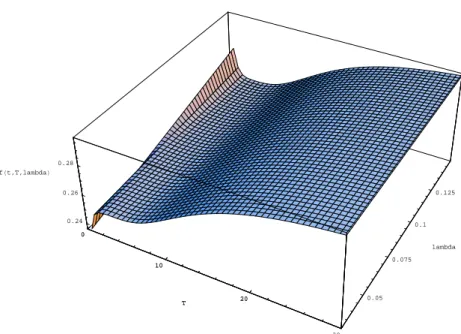
Figure 3.1 plots the forward rate (3.19) as function of the maturity T and the initial default intensity λ0 ∈ [0.03,0.15]. The net growth rate is η = 0.05, the
initial market price of risk is θ0 = 0.2. We have also used κ = 2, and ¯λ = 0.05,
σ = 0.15, mυ = 1, and h = 0.2. Furthermore, we assume that the short rate
evolves as a deterministic function of time namely drt=a(b−rt)dt, with a= 2, b = 0.06 and r0 = 0.08. Thus rt = e−at(r0 −b) +b. At the short end of the
forward rate curve the default-adjusted short rate dominates the market price of risk contribution, while at the long end the reverse holds true.
4
Monte Carlo Simulations
When dependence between the discounted GOP and the default-adjusted short rate is assumed, one can still evaluate the bond price using numerical techniques
0 10 20 30 T 0.05 0.075 0.1 0.125 lambda 0.24 0.26 0.28 fHt,T,lambdaL 0 10 20 T
Figure 3.1: Defaultable forward rate curves.
such as Monte Carlo simulation. We estimate the initial zero-coupon defaultable bond price from (3.4) by the means of Monte Carlo simulations by calculating
Pd(0, T) = ¯Q0E ¯ Sδ∗ 0 ¯ Sδ∗ T exp − Z T 0 rs+λsmυ ds |A0 , (4.1) where the discounted GOP ¯Sδ∗
t is driven by (3.8) and the jump intensityλtfollows
the dynamics (3.14), with E[dW˜t, dWt] =ρdt. Note that ¯Q0 = 1.
The challenge now lies on using an efficient simulation scheme. The standard discretisation schemes, for instance an Euler scheme, prove to be problematic. They allow the discounted GOP to take zero or even negative values, which results in meaningless prices. By using an exact simulation scheme, we can eliminate these problems. In Appendix D, we propose the exact simulation of two correlated squared Bessel processes as explained in Platen and Rendek (2009). Recall that the discounted GOP ¯Sδ∗
t is a time transformed squared Bessel process of dimension
four with some deterministic transformed time. The CIR type dynamics (3.14) of the jump intensity can be expressed as the product of a deterministic factor and a squared Bessel process.
The proposed Monte Carlo simulation method, especially when ρ 6= 0, requires substantial computational effort to be reasonably accurate. To significantly re-duce the statistical error of the simulation and consequently to minimise the computational effort, we discuss in the next subsection the effect of a variance re-duction method. More efficient variance rere-duction methods are available, see for instance Heath and Platen (2002b), but these more complex methods are beyond
the purpose of this work. Note that for ρ= 0, we obtain the special case studied in Section 3.2, which provides an explicit pricing formula for defaultable bond prices. We use this special case as control variate in the evaluation of defaultable bonds for the more general dependent case. This explicit pricing formula can be of great value also in other variance reduction methods.
4.1
Control Variate Method
To demonstrate that variance reduction can be efficiently improved, we consider Monte Carlo simulation using a control variate method. By concurrent Monte Carlo simulations of both the independent and the dependent case, the simulated bond prices are derived which are denoted as Pd
indep(0, T) and Pdepd (0, T),
respec-tively. We consider the outputs of N ∈ N Monte Carlo simulations. We denote
as I1,I2, . . . ,IN the outputs for the independent case and as D1,D2, . . . ,DN the
outputs for the more general dependent case. Then the bond price for the inde-pendent case is Pd
indep(0, T) =E[Ii] and the bond price for the dependent case is
Pd
dep(0, T) = E[Di], i∈ {1,2, . . . , N}. Denote as (D,I) a set of random variables
with the same distribution as (Di,Ii).
Under the assumption of independence between the discounted GOP and the default-adjusted short rate, the closed form bond prices (3.15) are obtained which are denoted asPd
analytic(0, T) and represent the explicitly known expectationE(I).
Then for any constant α, the sample mean
PCVd (0, T) = ¯D−α[¯I−E(I)] = 1 N N X i=1 (Di−α[Ii−E(I)]), (4.2)
is an unbiased estimator for Pd
dep(0, T). The optimal coefficient α, which
mini-mizes the variance of the unbiased estimator Pd
CV(0, T), is αmin = cov(I,D) var(I) = PN i=1(Ii−¯I)(Di−D¯) PN i=1(Ii−¯I)2 , (4.3)
see for instance Clewlow and Carverhill (1992). Because the optimal value of α
can only be approximated by estimating the quantities in (4.3), this will lead to an almost optimal control variate. For a study on minor effects on the efficiency of this kind of control variates see Lavenberg, Moeller, and Welch (1982).
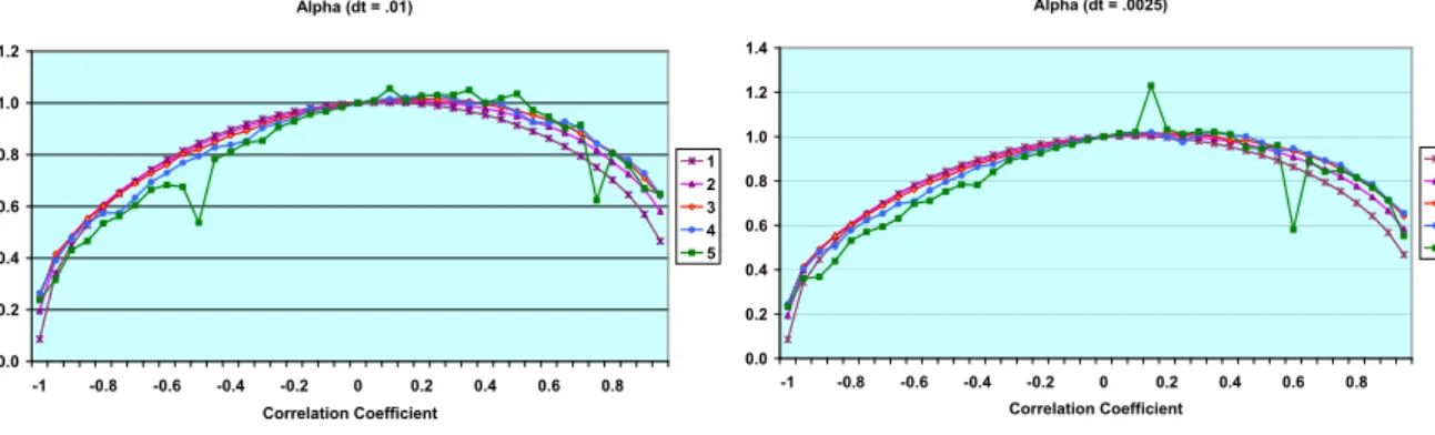
Figure 4.2 shows the effect of the correlation coefficient ρ on the value of α. For our simulations we have used a value ofα= 1, which seems reasonable, especially for |ρ| ≤0.5.
Figure 4.3 compares the standard error of the simulated prices of Pd
dep(0, T) and Pd
Alpha (dt = .01) 0.0 0.2 0.4 0.6 0.8 1.0 1.2 -1 -0.8 -0.6 -0.4 -0.2 0 0.2 0.4 0.6 0.8 Correlation Coefficient 1 2 3 4 5 Alpha (dt = .0025) 0.0 0.2 0.4 0.6 0.8 1.0 1.2 1.4 -1 -0.8 -0.6 -0.4 -0.2 0 0.2 0.4 0.6 0.8 Correlation Coefficient 1 2 3 4 5 Figure 4.2: α as a function of ρ
and that the initial market price of risk is |θ0|=
qα
0 ¯
Sδ∗
0
= 0.2, the net growth rate is η = 0.05 and T = 5. Furthermore we assume that the short rate evolves as a deterministic function of time namelydrt=a(b−rt)dt, with the same parameter
values as in Section 3.2.1. The parameter values of the default intensity (3.14) are ¯
λ = 0.05,σ = 0.15, α= 0.5,κ= 0.45 andh = 0.2. Note that for these parameter values, the squared Bessel process modelling the default intensity is of dimension four. We run two set of simulations, with N = 1,000,000 and N = 50,000,000 respectively. -6 -5 -4 -3 -2 0 0.1 0.2 0.3 0.4 0.5 0.6 0.7 0.8 0.9 1 Correlation Coefficient L o g ( S td E rr ) Dep 1,000,000 Dep 50,000,000 CV 1,000,000 CV 50,000,000
Figure 4.3: Log-log plot of the standard error for different correlation coefficients. Case “Dep”: Pd
dep(0, T). Case “CV”:PCVd (0, T).
Figure 4.3 demonstrates that for low correlation between the discounted GOP and the default intensity, the standard error of the bond price estimates using the control variate method are approximately one tenth the magnitude of the values obtained by simulation of the dependent model without variance reduction. This
reduction is uniform across the number of simulated paths and discretisation level. Thus, the same order of accuracy can be achieved by 100 times less the number of simulated paths. We confirm that by comparing the results for the different number of simulated paths, we observe that the results are consistent with the well-known fact that the standard errors decrease with 1/√N, at all reasonable discretization levels.
For ρ = 0.5, the 5−year bond prices estimated by the control variate method are of the order of at approximately one fifth with respect to the values obtained by the standard simulation scheme. However, for substantial correlation between the discounted GOP and the default intensity, for instance ρ = 0.9, the control variates have no significant effect. Similar results are obtained for the defaultable bond prices when parameters have been selected such that the squared Bessel process modelling the default intensity is of dimension three or five.
Note that there exists a variety of powerful variance reduction techniques that one can employ to further improve the efficiency of the Monte Carlo simulation, see for instance Kloeden and Platen (1999) and Heath and Platen (2002b), however, this is beyond the scope of this paper.
5
Conclusion
This paper presents alternative defaultable term structure models formulated in a general setting in which the existence of an equivalent risk-neutral probabil-ity measure is not required. The real-world dynamics of the defaultable forward rates and the defaultable bond price are obtained, as well as finite dimensional Markovian defaultable term structure models under separable volatility specifica-tions. Pricing in this general setting is accomplished by Monte Carlo simulation. Closed form solutions are derived under the assumption of independence between the discounted GOP and the default intensity, which turn out to be very usefull in this context. These can serve as control variates for variance reduction methods, which can significantly reduce the standard error of the Monte Carlo simulation for the more general models.
The proposed modelling approach holds great potential for more accurate credit risk assessment and measurement. It is a consistent approach under which pricing, hedging and credit risk measurement can be performed under a unique probability measure, the real-world probability measure. Therefore, we are able to perform a type of absolute pricing which has the significant advantage of estimating prices that reflect historical information and economic reasoning and not the common type of relative pricing. Real-world default probabilities can be evaluated by observed credit spreads, a feature that makes pricing and risk measurement more reliable and opens a line of further research.
Acknowledgement
The authors would like to thank Carl Chiarella for his valuable comments. Fur-thermore, we would like to thank Troy Morgan for his significant contribution to the development of the numerical simulations.
A
Appendix: Proof of Proposition 2.2
Let us define a “pseudo” zero-coupon bond ˜P(t, T), fort ∈[0, T] and T ∈[0,T¯], ¯
T ∈[0,∞), which will be used in the following proofs. The pseudo zero-coupon bond ˜P(t, T) is the price of a defaultable zero-coupon bond maturing atT, which is identical to the defaultable bond P(t, T), but has not defaulted up to time t. Then ˜ P(t, T) = exp − Z T t fd(t, s)ds , (A.1)
and thus the value of the defaultable bond Pd(t, T) (2.18) is given by
Pd(t, T) = ˜P(t, T) ¯Qt. (A.2)
Using the dynamics (2.8) and (2.12), an application of the Itˆo formula derives the dynamics of the pseudo zero-coupon bond ˜P(t, T) as
dP˜(t, T) = ˜P(t−, T) " rt+ m X i=1 ˜ σi(t, T)θit + Z 1 0 [(1−v) ˜β(v, t, T)−v](ψ(v, t)−1)φ(dv, t) dt + m X i=1 ˜ σi(t, T)dWi t + Z 1 0 ˜ β(v, t, T)p(dv, dt) # , (A.3) for all t ∈[0, T], with
˜ σi(t, T) = σi(t, T), (A.4) and ˜ β(v, t, T) = β(v, t, T) +v 1−v = βM(v, t, T) 1−v . (A.5)
From the real-world dynamics (2.11) of the benchmarked defaultable bond price and the Itˆo formula, we obtain
dln( ˆPd(t, T)) = − m X i=1 1 2(ˆσ i(t, T))2dt+ ˆσi(t, T)dWi t (A.6) + Z 1 0 ˆ β(v, t, T) + ln(1−βˆ(v, t, T))φ(dv)dt+ Z 1 0 ln1−βˆ(v, t, T)q(dv, dt).
Using definition (2.19) and (A.6), the defaultable forward rate dynamics under the real-world probability measure are
dfd(t, T) = m X i=1 ∂ ∂Tˆσ i(t, T) ˆσi(t, T)dt+dWi t (A.7) + Z 1 0 ∂ ∂Tβˆ(v, t, T) 1−βˆ(v, t, T) ˆ β(v, t, T)φ(dv)dt+q(dv, dt),
for t ∈[0, T]. Next we express the dynamics of the forward rates (A.7) in terms of the diffusion coefficients (2.22) and the jump coefficient (2.23), where we have
Z T t σdi(t, s)ds= ˆσi(t, T)−σˆi(t, t), (A.8) Z T t βd(v, t, s)ds=−ln 1−βˆ(v, t, T) 1−βˆ(v, t, t) ! . (A.9)
However, the “pseudo” bond volatilities (A.4) and (A.5) must satisfy the condi-tions (by definition (A.1), we have that ˜P(t, t) = 1, for t∈[0, T])
0 = ˜σi(t, t) = σi(t, t),
0 = ˜β(v, t, t) = β(v, t, t) +v 1−v .
Using (2.13) and (2.14) we obtain that
σi(t, t) =θti−σˆi(t, t) = 0, β(v, t, t) = ψ(v, t)−βˆ(v, t, t) 1−ψ(v, t) =−v, therefore ˆ σi(t, t) =θti, ˆ β(v, t, t) =ψ(v, t) + (1−ψ(v, t))v.
By (A.8) and (A.9), the benchmarked defaultable bond volatilities are linked to the defaultable forward rate volatilities by the relations
ˆ σi(t, T) = Z T t σdi(t, s)ds+θit, (A.10) ˆ β(v, t, T) = 1−exp − Z T t βd(v, t, s)ds (1−ψ(v, t))(1−v), (A.11) which yields (2.20).
B
Appendix: Proof of Equation (2.25)
By equation (2.20), which we recall here
dfd(t, T) =µ d(t, T)dt+ m X i=1 σi d(t, T)dWti+ Z 1 0 βd(v, t, T)p(dv, dt), (B.1)
and by using Proposition 2.2 of Bj¨ork, Kabanov, and Runggaldier (1997), we obtain the dynamics of the “pseudo” zero-coupon bond price ¯P(t, T), defined in (A.1), as dP¯(t, T) = ¯P(t−, T) " rdt − Z T t µd(t, u)du+ m X i=1 1 2 Z T t σdi(t, u)du 2! dt − m X i=1 Z T t σi d(t, u)dudWti− Z 1 0 1−exp − Z T t βd(v, t, u)du p(dv, dt) # . (B.2) Note that the defaultable spot rate rd
t is defined as rdt = fd(t, t), for all t ∈
[0, T]. By comparison with the dynamics of the “pseudo” zero-coupon bond price obtained in (A.3), we derive the following relationships
¯ σi(t, T) = − Z T t σi d(t, u)du, (B.3) ¯ β(v, t, T) = −1 + exp − Z T t βd(v, t, u)du , (B.4)
and the drift term ¯µ(t, T) is given by ¯ µ(t, T) =rtd− Z T t µd(t, u)du+ m X i=1 1 2 Z T t σdi(t, u)du 2 , (B.5) with (see (A.3))
¯ µ(t, T) =rt+ m X i=1 ¯ σi(t, T)θti+ Z 1 0 [(1−v) ¯β(v, t, T)−v](ψ(v, t)−1)φ(dv). (B.6) Using the relations (A.4), (2.13) and (A.10) we confirm that (B.3) holds since ¯ σi(t, T) =σi(t, T) =θti−σˆi(t, T) = θit−( Z T t σdi(t, s)ds+θit) = − Z T t σdi(t, s)ds.
Similarly, by using (A.5), (2.14) and (A.11) β(v, t, T) = ψ(v, t)−βˆ(v, t, T) 1−ψ(v, t) = ψ(v, t)−1 + exp−RT t βd(v, t, s)ds (1−ψ(v, t))(1−v) 1−ψ(v, t) =−1 + exp − Z T t βd(v, t, s)ds (1−v).
Thus we confirm (B.4) since ¯ β(v, t, T) = β(v, t, T) +v 1−v =−1 + exp − Z T t βd(v, t, u)du .
From (B.3), (B.4), (B.5) and (B.6) we express the short rate spread as
rtd−rt= Z T t µd(t, u)du− m X i=1 1 2 Z T t σid(t, u)du 2 + m X i=1 ¯ σi(t, T)θit+ Z 1 0 [(1−v) ¯β(v, t, T)−v](ψ(v, t)−1)φ(dv) = Z T t µd(t, u)du− m X i=1 1 2 Z T t σid(t, u)du 2 (B.7) − m X i=1 θit Z T t σdi(t, s)ds+ Z 1 0 [(1−v)e−RtTβd(v,t,u)du−1](ψ(v, t)−1)φ(dv).
By using the drift restriction (2.21)
Z T t µd(t, u)du= m X i=1 Z T t σdi(t, u) Z u t σid(t, s)ds+θti du − Z T t Z 1 0 βd(v, t, u) exp − Z u t βd(v, t, s)ds (1−ψ(v, t))(1−v)φ(dv)du, = m X i=1 Z T t σdi(t, u) Z u t σdi(t, s)dsdu+ m X i=1 θti Z T t σdi(t, u)du (B.8) − Z T t Z 1 0 βd(v, t, u) exp − Z u t βd(v, t, s)ds (1−ψ(v, t))(1−v)φ(dv)du. Note that Z T t σdi(t, u) Z u t σdi(t, s)dsdu= 1 2 Z T t ∂ ∂u Z u t σdi(t, s)ds 2 ds = 1 2 Z T t σdi(t, u)du 2 . (B.9)
Note also that Z T t Z 1 0 βd(v, t, u) exp − Z u t βd(v, t, s)ds (1−ψ(v, t))(1−v)φ(dv)du = Z 1 0 (1−ψ(v, t))(1−v) Z T t βd(v, t, u) exp − Z u t βd(v, t, s)ds duφ(dv) = Z 1 0 (1−ψ(v, t))(1−v) exp − Z T t βd(v, t, s)ds −1 φ(dv). (B.10) Thus by (B.7), (B.8), (B.9) and (B.10) we obtain that
rdt −rt= Z 1 0 (1−ψ(v, t))(1−v)he−RtTβd(v,t,s)ds−1 i φ(dv) + Z 1 0 [(1−v)e−RtTβd(v,t,u)du−1](ψ(v, t)−1)φ(dv). = Z 1 0 (1−ψ(v, t))vφ(dv). (B.11)
C
Appendix: Proof of Proposition 2.4
Using the dynamics of the forward rate (2.20), and setting t=T, we can use the identity rd
t =fd(t, t) to obtain the short rate dynamics rtd=fd(0, t) + Z t 0 µd(u, t)du+ m X i=1 Z t 0 σdi(u, t)dWui+ Z t 0 Z 1 0 βd(v, u, t)p(dv, du), (C.1) with µd as in (2.21). Thus drdt = ∂ ∂Tf d( t, T)|T=tdt+dfd(t, T)|T=t = " ∂ ∂Tf d (0, T)|T=t+ Z t 0 ∂ ∂Tµd(u, T)|T=tdu+ m X i=1 Z t 0 ∂ ∂Tσ i d(u, T)|T=tdWui + Z t 0 Z 1 0 ∂ ∂Tβd(v, u, T)|T=tp(dv, du) dt +µd(t, t)dt+ m X i=1 σid(t, t)dW i t + Z 1 0 βd(v, t, t)p(dv, dt). (C.2)
Using the volatility specifications of Assumption 2.3, we obtain
∂σi d(u, T)
∂T |T=t =−k
i
and ∂βd(v, u, T) ∂T |T=t=−kβ(t)βd(v, u, t). (C.4) By introducing Vσi(u, T) =σdi(u, T) Z T u σdi(u, s)ds, (C.5) and Vβ(v, u, T) = (1−v)βd(v, u, T) exp − Z T u βd(v, u, s)ds , (C.6) we have by (2.21) that µd(u, T) = m X i=1 Vσi(u, T) + m X i=1 σid(u, T)θui − Z 1 0 Vβ(v, u, T)(1−ψ(v, u))φ(dv, t). (C.7) Also note that by (2.27), for i∈ {1,2, . . . , m},
∂Vi σ(u, T) ∂T |T=t =−k i σ(t)Vσi(u, t) + (σdi(u, t))2, (C.8) and by (2.28) ∂Vβ(v, u, T) ∂T |T=t =−kβ(t)Vβ(v, u, t)−(1−v)(βd(v, u, t)) 2e−Rt uβd(v,u,s)ds. (C.9)
Using the above results, the dynamics of the spot rate (C.2) are expanded to drtd= ( ∂ ∂Tf d (0, T)|T=t+ Z t 0 m X i=1 −kσi(t)V i σ(u, t) + (σ i d(u, t))2−k i σ(t)σ i F(u, t)θ i u du + Z t 0 Z 1 0 hn kβ(t)Vβ(v, u, t) + (1−v)(βd(v, u, t))2e− Rt uβd(v,u,s)ds o (1−ψ(v, u))φ(dv, t)idu − m X i=1 ki σ(t) Z t 0 σi d(u, t)dWui−kβ(t) Z t 0 Z 1 0 βd(v, u, t)p(dv, du) ) dt (C.10) + m X i=1 σid(t, t)θ i t− Z 1 0 βd(v, t, t)(1−v)(1−ψ(v, t))φ(dv, t) ! dt + m X i=1 σi d(t, t)dWti+ Z 1 0 βd(v, t, t)p(dv, dt).
By using the definitions (2.30), (2.31), (2.32) and (2.33), (C.10) reduces to
drdt = ( ∂ ∂Tf d(0, T) |T=t+Eβ(t) + m X i=1 Eσi(t)− m X i=1 kσi(t)Dσi(t)−kβ(t)Dβ(t) + m X i=1 ¯ σid(t,Ft)θit ) dt+ m X i=1 ¯ σid(t,Ft)dWti+ Z 1 0 ¯ βd(v, t)p(dv, dt). (C.11)
Further from definitions (2.31) and (2.32), (C.1) yields Dσ1(t) =rtd−fd(0, t)− m X i=2 Dσi(t)− Dβ(t), (C.12) which reduces (C.11) to (2.29).
D
Simulation of Correlated Squared Bessel
Pro-cesses
The objective is to simulate the discounted GOP and the default adjusted short rate by allowing correlated dynamics. The dynamics (3.8) drive the discounted GOP, recall
dS¯δ∗
t = ¯Stδ−∗θt(θtdt+dWt), (D.1)
with the net market trend defined by
αt= ¯Stδ∗|θt|2. (D.2)
Note that the total market price of risk can be expressed as
|θt|= rα t ¯ Sδ∗ t , (D.3)
and the dynamics (D.1) are
dS¯δ∗
t =αtdt+
q
αtS¯tδ∗dWt. (D.4)
By introducing the transformed time ϕ1
t satisfying dϕ1t = 1 4 Z t 0 αsds, (D.5)
then the process Xϕ1 t = ¯S δ∗ t has dynamics dXϕ1 t =4dϕ 1 t + 2 q Xϕ1 tdW(ϕ 1 t), (D.6) where dW(ϕ1 t) = pαt
4dWt. This is the SDE of a square Bessel process of
di-mension 4. Under the MMM proposed by Platen (2001) and Platen (2002), a deterministic time transformation is assumed with the net market trend αt, t ∈[0, T] having the form
where η > 0 is the constant net growth rate and α0 > 0 is an initial scaling
parameter. Then the transformed time is reduced to
ϕ1t =ϕ10+α0 4η(e
ηt
−1). (D.8)
(ϕ1
0 = 0) Next consider the normalised GOP
Yt= ¯ Sδ∗ t αt , (D.9)
for t∈[0,∞). Then by the Itˆo formula we obtain
dYt=(1−ηYt)dt+ p YtdWt, (D.10) for t ∈ [0,∞) and Y0 = ¯ Sδ∗ 0
α0 . Therefore from (D.9), the discounted GOP can be
expressed as the product of the exponential function (D.7) and the square root process (D.10).
The stochastic jump intensity λt follows the dynamics (3.14) recall dλt=κ λ¯−λt
dt+σpλtdW˜t+dJt, (D.11)
where κ,¯λ, σ are positive constants, with 2κλ > σ¯ 2. Between the jump times, we
need to simulate the continuous part of these dynamics, namely
dλt=κ λ¯−λt
dt+σpλtdW˜t. (D.12)
Let us introduce the exponential function st
st=s0exp (−κ t), (D.13)
and the transformed time
ϕ2t =ϕ20+1 4 Z t 0 σ2 su du=ϕ20+ σ 2 4κ s0 (exp (κ t)−1). (D.14) Then the square root process (D.12) can be expressed as the product of the exponential function (D.13) st and the squared Bessel process ˜X of dimension δ = 4σκ2¯λ >0 by the transformation
λt=stX˜ϕ2
t, (D.15)
for t∈[0,∞). Note that
dX˜ϕ2 t =δdϕ 2 t + 2 q ˜ Xϕ2 td ˜ W(ϕ2t), (D.16) where dW˜(ϕ2 t) = q σ2 4std ˜ Wt.
We illustrate next the simulation of these two correlated squared Bessel processes. Recall that E[dW˜t, dWt] =ρdt. The discounted GOP is a squared Bessel process
of dimension 4 and we assume that the default adjusted short rate is a squared Bessel process of dimension δ ∈ {1,2,3, . . .}. In general the dimension δ can be any nonnegative real number, however we restrict it to an integer to be able to simulate two correlated squared Bessel processes as explained in Renata and Platen. Motivated by the 2 ×2 matrix time changed Wishart process where the diagonal elements of the process formulate correlated time changed squared Bessel processes of the same dimension, we consider a more general setting. We consider the two time changed matrix Wiener processes Wϕ1
t = [W ij ϕ1 t] 4,2 i,j=1 with ϕ1 t defined by (D.8) andW˜ϕ2 t = [ ˜W i,j ϕ2 t] δ,2
i,j=1 withϕ2t defined by (D.14). Renata and
Platen have illustrated that correlated time changed squared Bessel processes can be constructed as follows: ¯ Sδ∗ t =Xϕ1 t = ( Pδ i=1(wi,1+̺W i,1 ϕ1 t + p 1−̺2Wi,2 ϕ1 t) 2 +P4 i=δ+1(wi,1+W i,1 ϕ1 t), δ≤4; P4 i=1(wi,1+̺W i,1 ϕ1 t + p 1−̺2Wi,2 ϕ1 t) 2, δ > 4. (D.17) and λt st = ˜Xϕ2 t = δ X i=1 (wi,2+ ˜Wϕi,21 t) 2, (D.18)
where X0 = P4i=1(wi,1)2 and ˜X0 = Pδi=1(wi,2)2. This setup depends on the
dimension δ of the squared Bessel process modelling the default adjusted short rate.
Let consider the time t = {t0, t1, . . . , tN = T}, then the time ϕt is defined as ϕt={ϕt0, ϕt1, . . . , ϕT}, where ϕtis determined here by (D.8) or (D.14). Theϕ−
time increment is ∆ϕ =ϕti−ϕti−1, therefore
Wϕit =Wϕi−t1+p∆ϕx, withx∼N(0,1). (D.19)
For instance if thet−time increment is ∆ = T
N, then thet={0,∆,2∆, . . . , N∆ = T}, and the ϕt={ϕ0, ϕ∆, ϕ2∆, . . . , ϕT}, therefore ∆ϕ =ϕi∆−ϕ(i−1)∆.
References
Albanese, C. and O. X. Chen (2005). Discrete credit barrier models. Quanti-tative Finance 5(3), 247–256.
Bj¨ork, T., Y. Kabanov, and W. Runggaldier (1997). Bond market structure in the presence of market point processes. Mathematical Finance 7, 211–239. Broadie, M. and O. Kaya (2006). Exact simulation of stochastic volatility and other affine jump diffusion processes. Operations Research 54(2), 217–231. Bruti-Liberati, N., C. Nikitopoulos-Sklibosios, and E. Platen (2007). Pricing under the real-world probability measure for jump-diffusion term struc-ture models. Technical report, University of Technology, Sydney. QFRC Research Paper 198, Quantitative Finance to appear.
Chiarella, C., E. Schl¨ogl, and C. S. Nikitopoulos (2007). A Markovian Default-able Term Structure Model with State Dependent Volatilities.International Journal of Theoretical and Applied Finance 10(1), 155–202.
Christensen, M. M. and E. Platen (2005). A general benchmark model for stochastic jump sizes. Stochastic Analysis and Applications 23(5), 1017– 1044.
Clewlow, L. and A. Carverhill (1992). Efficient Monte Carlo valuation and hedging of contingent claims. Technical report, Financial Options Research Centre, University of Warwick. 92/30.
Duffie, D. (2005). Credit risk modelling with affine processes.Journal of Bank-ing and Finance 29, 2751–2802.
Duffie, D. and K. Singleton (1999). Modeling term structures of defaultable bonds. Review of Financial Studies 12, 687–720.
Elliott, R. J., M. Jeanblanc, and M. Yor (2000). On models on default risk.
Mathematical Finance 10(2), 179–196.
Filipovi´c, D. (2001). A general characterization of one factor affine term struc-ture models. Finance and Stochastics 5, 389–412.
Heath, D., R. Jarrow, and A. Morton (1992). Bond pricing and the term struc-ture of interest rates: A new methodology for contingent claim valuation.
Econometrica 60(1), 77–105.
Heath, D. and E. Platen (2002a). Perfect hedging of index derivatives under a minimal market model. International Journal of Theoretical and Applied Finance 5(7), 757–774.
Heath, D. and E. Platen (2002b). A variance reduction technique based on integral representations. Quantitative Finance 2(5), 362–369.
Karatzas, I. and S. E. Shreve (1998). Methods of Mathematical Finance, Vol-ume 39. Springer.
Kelly, J. R. (1956). A new interpretation of information rate. Bell System Technical Journal 35, 917–926.
Kloeden, P. E. and E. Platen (1999). Numerical Solution of Stochastic Differ-ential Equations, Volume 23. Springer. Third corrected printing.
Lavenberg, S., T. Moeller, and P. Welch (1982). Statistical results on con-trol variables with application to queueing network simulation. Operations Research 30, 182–202.
Long, J. B. (1990). The numeraire portfolio. Journal of Financial Eco-nomics 26, 29–69.
Matacz, A. and J. P. Bouchaud (2000). An empirical investigation of the for-ward interest rate term structure. International Journal of Theoretical and Applied Finance 3(4), 703–729.
Platen, E. (2001). A minimal financial market model. InTrends in Mathemat-ics, pp. 293–301. Birkh¨auser.
Platen, E. (2002). Arbitrage in continuous complete markets.Advances in Ap-plied Probability 34(3), 540–558.
Platen, E. (2005). An alternative interest rate term structure model. Interna-tional Journal of Theoretical and Applied Finance 8(6), 717–735.
Platen, E. and D. Heath (2006). A Benchmark Approach to Quantitative Fi-nance. Springer.
Platen, E. and R. Rendek (2009). Exact scenario simulation for selected multi-dimensional stochastic processes. UTS (working paper).
Sch¨onbucher, P. J. (1998). Term structure modelling of defaultable bonds. Re-view of Derivatives Research 2, 161–192.
Sch¨onbucher, P. J. (2003). Credit Derivatives Pricing Models. Wiley, Chich-ester.