Improving EV Lateral Dynamics Control Using Infinity Norm Approach with Closed-form Solution

Improving EV Lateral Dynamics Control Using

Infinity Norm Approach with Closed-form Solution

Alexander Viehweider

Dept. of Advanced Energy The University of Tokyo, 5-1-5 Kashiwanoha, Kashiwa, Chiba, Japan

Email: [email protected]

Valerio Salvucci, Yoichi Hori, Takafumi Koseki

Dept. of Electrical Engineering University of Tokyo, 3-7-1 Hongo Bunkyoku Tokyo, Japan

Email: [email protected], [email protected], [email protected]

Abstract—Over-actuated EVs offer a high degree of freedoms that can be exploited for better vehicle dynamic behaviour, energy efficiency, vehicle safety and comfort. If the cost of the actuators can be brought to a reasonable level, then sophisticated control algorithm should make the most out of the over-actuation property.

A key aspect in lateral dynamics control of an over actuated EV with In Wheel motors and active front and/or rear steering is the so called control allocation problem. Often such problems are solved using the 2 norm (weighted least square solution) as it is expressed in a closed form-solution and has a low fixed number of arithmetic operations suited for real time control. In this work a closed-form solution based on the infinity norm for the case of 2 to 3 control allocation problem in EV lateral dynamic control is derived, and validated by means of simulation runs considering an electric vehicle with In-Wheel-Motor traction and active front and rear steering. During a ”sine with a dwell” steering command at a constant velocity the superiority of the proposed algorithm based on the infinity norm is shown.

I. INTRODUCTION

Over-actuated systems have an intrinsic redundancy ex-ploited for fault robustness and in the case that all actua-tors work properly for optimizing some other property of the system (energy consumption, limiting maximal actuator power ...). They appear in nearly all engineering disciplines. Mechatronic examples are airplanes [1], bi-articularly actuated robots [2], and electric vehicles with In-Wheel-Motors [3] with/without active front and rear steering [4], [5].

As a consequence of redundancy in actuation, a control allocation problem arises in all these applications. Tradition-ally the 2 norm is used to resolve such problem, due to the fact that it allows to write a solution in a closed form solution. For certain specific problems, such as the actuator redundancy resulting from bi-articular actuation in robot arms [6], a closed-form solution based on the infinity norm is possible, and its higher performances in respect to the 2 norm in terms of output maximization have been shown [7], [8].

In this work, lateral dynamic control for EV is considered. A closed-form solution based on the∞norm for the 2 outputs to 3 inputs control allocation problem in EV lateral dynamic control is derived, and its higher performances in respect to the traditional 2 norm based algorithm are investigated.

In Sec. II the vehicle lateral dynamics modeling and allo-cation problem is described. In Sec. III the traditional 2 norm

based and the proposed∞norm based models for resolving the 2 to 3 allocation problem are shown. In Sec. IV the simulation results are analyzed and discussed. Finally, the advantages of the proposed algorithm are summarized in Sec. V.

II. EV LATERALDYNAMICSCONTROL

EVs offer apart from their particular energy source the opportunity to install in each wheel a motor, therefore in-troducing new degrees of freedom in the vehicle dynamic control design [9], [10]. In this contribution the opportunity to generate an additional yaw moment Mz by appropriate single wheel torque commands is exploited. Compared to conventional cars [11] the yaw momentMz can be generated quite easily by a EV with In-Wheel-Motors. Additionally, it is assumed that front and rear steering are active, meaning that front and rear steering are influenced by the control system and are not strictly coupled with handwheel steering angle. Such vehicles do already exist as test vehicle in laboratories [12].

A. Vehicle lateral dynamics modelling

The linear bicycle model in the case of an In-Wheel-Driven Electric Vehicle with Active Front and Rear steering in the case of constant vehicle longitudinal velocity vx (As far as the influence of longitudinal forces in contributing to the overall lateral forces due to the steering angle is concerned, we consider this influence as model uncertainty.) is as follows [13]: ˙x = Ax+v∗=Ax+Bu∗ _˙ β ˙ γ =   −(Cf+Cr) mvx lrCr−lfCf mv2 x −1 lrCr−lfCf Jz − lr2Cr+l2fCf Jzvx   β γ + + " Cf mvx Cr mvx 0 lfCf Jz − lrCr Jz 1 Jz #  δf δr Mz  , (1)

whereCf,Cr are the front and rear cornering stiffness values,

m,Jz the vehicle mass and the vehicle yaw inertia, lf,lr the distance from the front and rear axle to the center of gravity andδf,δr,Mz the front steering angle,the rear steering angle and the additional yaw moment respectively. Three inputs are used to determine the two states (body slip angle β and yaw

Fyf Fyr ay Fw ϒ δf δr lf lr lw v β δT vT αT

T

Fig. 1. Bicycle model (left) with combined front lateral and rear lateral tire forces and definition of tire slip angleα(right). (ay: lateral acceleration,γ: yaw rate,β: body slip angle,δf: front steering angle,δr: rear steering angle, Fy f: combined front lateral tire force,Fyr: combined rear lateral tire force, Fw: wind disturbance force,lf: distance of front axle from COG,lr: distance

of rear axle from COG ,lw: distance of aerocenter from COG).

rate γ). This means it is an over actuated system and control allocation problem of the type 2 to 3.

The model (1) describes the vehicle in the linear domain of operation. It assumes that the steering anglesδf,δr and the tire slip anglesαf,αr are small. However under certain operation condition the EV enters the non linear domain of operation. The allocation scheme should help to keep the EV in the linear domain of operation.

B. Vehicle lateral dynamics control and allocation problem

A control system for lateral vehicle dynamics is established as shown in Fig. 2. The controller tries to track the yaw rate

γ and the body slip angle β of the vehicle. It is assumed

that these two quantities are measured/observed. This may be difficult as far as the body slip angleβ is concerned. However,

this estimation problem is not part of this contribution, we refer to [14]. The controller computes a two dimensional virtual controller output v∗ which is mapped by using an infinity norm criteria and the allocation equation to a three dimensional actuator demandu∗(true controller output) :

v∗=Bu∗ (2) with B= " Cf mvx Cr mvx 0 Cflf Jz −Crlr Jz 1 Jz # ,u∗=   δf δr Mz  . (3)

In the following we assume a linear relationship between the tire slip angles αf, αr and the steering angles δf, δr as follows:

αf =δf−β−

lf

vx

γ (4)

Fig. 2. Overview of the considered control system. The controller computes a virtual control input which is translated by the control allocator to the true control input. It is assumed that the vehicle yaw rateγand the body slip angle βcan be measured or observed.

Fig. 3. Instead of allocating the front and rear steering angles directly, the allocator outputu1,u2 are the front and rear tire slip angles which are translated to the steering angles. By doing so the bounds in the allocation can be kept constant.

αr=δr−β+lr vx

γ (5)

Since the value of the tire slip anglesαf,αr are to be kept small and not necessarily the steering anglesδf,δr in order to keep the vehicle in the linear range of operation (stable) and in order to avoid time variant bounds as maximal values in the allocation equation we decompose the allocated variable (actuator demand):

u∗=u0+u, (6)

where u0 corresponds to the actuator demand corresponding

to zero tire slip angles:

u0(t) =    β(t) +_vlf xγ(t) β(t)−_vlr xγ(t) 0   . (7)

With the decomposition (Fig. 3) of the actuator demand the allocation problem is formulated as following:

v=Bu. (8)

By combining (2), (6) and (8) it follows:

v=v∗−Bu0. (9)

The entry u1 and u2 of the vectoru= [u1,u2,u3]T can be directly interpreted as the front and rear lateral tire slip angle

Taking into account (8), givenuit is possible to determinev uniquely. On the other hand, givenvit is generally not possible to determine uniquely u due to the actuator redundancy. The problem represented by (8) is referred in the following as 2 outputs to 3 inputs control allocation problem. The vector u= [u1,u2,u3]T in this contribution is also referred as true controller output and the vector v= [v1,v2]T as virtual controller output and

B= b11 b12 b13 b21 b22 b23 (10) as allocation matrix.

III. 2OUTPUTS TO3INPUTS ALLOCATION RESOLUTION To determine a specific solution from the infinite number of solutions due to the actuation redundancy an optimization criteria must be used. The most used criteria is the (weighted) least square problem (2 norm), mainly because the solution is expressed by a closed-form expression (using the pseudo inverse). However, the least square solution does not exploit the available actuation range very well [6]. In contrast, op-timization criteria based on ∞ norm allow the use of all the solution space, but usually the solution is determined using iterative algorithms. As a consequence, to have a closed-form solution based on the ∞norm is highly advantageous.

A. 2 norm based approach

The 2 to 3 allocation problem is resolved using the 2 norm by solving the following problem:

min r (u₁)2 (um 1)2 +(u2)2 (um 2)2 +(u3)2 (um 3)2 s.t. v=Bu (11)

The solution of the problem expressed by (11) is obtained using a generalized pseudo inverse:

u_opt=W−1BT(BW−1BT)−1v (12) where W=diag( 1 (um₁)2, 1 (um₂)2, 1 (um₃)2). (13)

B. Infinity norm based approach

The 2 to 3 allocation problem is resolved using the∞norm by solving the following problem:

min max|u1| um₁ , |u2| um₂ , |u3| um₃ s.t. v=Bu (14)

The objective function is weighted, that is the three input valuesuifor(i=1,2,3)are scaled by the respective maximum valueum

i for(i=1,2,3). By doing so the entire solution space −um_i ≤u_i≤u_im, fori=1,2,3 (15) is exploited efficiently as shown in III-C.

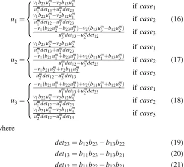
A closed form solution of the problem (14) is represented by three functions, each one expressed with a three piecewise linear function: u₁=        v1b23um1−v2b13um1

um₁det13+um2det23 if case1

v1b22um1−v2b12um1

um

1det12−um3det23 if case2 −v1(b22um2−b23um3)−v2(b13um3−b12um2)

um₃det13−um2det12 if case3

(16) u₂=        v1b23um2−v2b13um2

um₁det13+um2det23 if case1 −v1(b21um1+b23um3)+v2(b11um1+b13um3)

um₁det12−um3det23 if case2 −v1b21um2+v2b11um2

um

2det12−um3det13 if case3

(17) u₃=        −v1(b21um1+b22um2)+v2(b11um1+b12um2)

um₁det13+um2det23 if case1

v1b22um3−v2b12um3

um₁det12−um3det23 if case2

v1b21um3−v2b11um3

um

2det12−um3det13 if case3

(18) where det23=b12b23−b13b22 (19) det13=b11b23−b13b21 (20) det12=b11b22−b12b21 (21) and case1=(kv21v2≤kv11v1 andkv22v2≥kv12v1)or (kv21v2≥kv11v1 andkv22v2≤kv12v1) case2=(kv21v2≤kv11v1 andkv23v2≥kv13v1)or (kv21v2≥kv11v1 andkv23v2≤kv13v1) case3=(kv22v2≤kv12v1 andkv23v2≤kv13v1)or (kv22v2≥kv12v1 andkv23v2≥kv13v1) where kv11= (b21um1+b22um2+b23um3) (22) kv12= (b21um1+b22um2−b23um3) (23) kv13= (b21um1−b22um2+b23um3) (24) kv21= (b11um1+b12um2+b13um3) (25) kv22= (b11um1+b12um2−b13um3) (26) kv23= (b11um1−b12um2+b13um3) (27) Equations (16), (17), and (18) are derived following the same method used in [6]. They are continuous in all the domain

D= (v₁,v₂)under the condition that all the denominators are different from 0 (satisfied forB andum in this work).

C. Infinity Norm Approach: the Reason Why

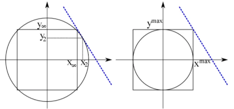
Fig. 4 shows the graphical comparison between∞norm and 2 norm optimization criteria in selecting the optimal solution for a problem in R2. The dashed line represents the infinite set of solutions (x,y)that satisfy,

k=αx+y (28)

whereα represents the relationship between the desired output kand the necessary inputsxandy. The positive constantsxmax

Fig. 4. Graphical comparison between ∞ norm and 2 norm: solution comparison (left), no solution for 2 norm (right)

andymax define the allowable ranges forxandy:

−xmax≤x≤xmax (29)

−ymax≤y≤ymax (30)

The two sets (x2,y2) and (x∞,y∞) in Fig. 4 (left) are the two solutions of (28) calculated using the 2 norm (the circle) and ∞ norm (the square) optimization criteria, respectively. By definition, the infinity norm minimize the maximum input, therefore it holds:

max{|x∞|,|y∞|} ≤max{|x2|,|y2|} (31) Therefore, if x and y are bounded as in (29) and (30), the ∞norm model admits solution for higher values ofkthan the 2 norm, as shown in Fig. 4 (right). The greater solution space of the∞norm model holds also inR3, the mathematical space of the redundancy resolution problem in this work.

IV. SIMULATION ANDRESULTS

Advantages by using the∞norm are now shown by consid-ering an EV at constant velocity carrying out a ”sine with a dwell” steering command. The simulation runs have been car-ried out with the professional simulation environment CarSim. A highly sophisticated CarSim vehicle model has been used that considers explicitly the different side slip angles at the four wheels, load transfer, suspension effects and a complex non linear tyre model including tire dynamics. Whereas the control design has been based on a highly simplified model of the vehicle dynamics as shown in (1), the overall system simulation used the aforementioned sophisticated CarSim ve-hicle model. The parameters are set in the following way: mass

m=830 kg, yaw inertiaJz=562 kgm2 and front (rear) axle distance from the center of gravitylf=0.999m(lr=0.701m) has been considered. The vehicle is assumed to be running on a slightly slippery road with µ=0.7 and the driver to give a

sine with a dwell steering command as depicted in Fig. 5. As controller a sliding mode controller as described in [4] has been used, the controller parameter (gains) have been set once and left untouched during all simulation runs. The controller gets reference values which are derived from the

Fig. 5. Steering command signal δsteer ”sine with a dwell” used for the

simulation series. The maximal steering angle δmax is varied during the

simulation runs.

”sine with a dwell” steering command:

γre f = vx (lf+lr)(1+ v 2 x v2_ch) δsteer (32)

wherevchis the characteristic velocity of the car. The reference for the body slip angle has been set to zero, βre f=0◦.

Two allocation methods have been compared. The first is the weighted means square solution according to (11) and the second one is the weighted infinity norm according to (14) with the closed form solution as described in III-B. Both methods have been embedded in the scheme of Fig. 3 where the tire slip anglesαf,αrare allocated by the allocation algorithm instead of the steering angles and after the allocation translated to the steering angles δf,δr by use of (4), (5) and (6) since the body slip angleβ, the yaw rateγ and the velocity vxare assumed to be known. The torque momentMz has been evenly distributed to the 4 wheels. The tire slip angle maximal valuesum₁,um₂ have been set to 5◦for front and rear tire slip. The torque moment valueum₃ has been set to 2000Nm. Without further knowledge of these bounds this seems to be reasonable. The inclusion of online estimation of these bounds is not topic of this contribution, it is referred to [15], [16], [17]. Additionally geometric constraints for the steering angles have been considered in the simulation (δf,max=17◦,δr,max=4.5◦). In Fig. 6 and Fig. 7 the steering manoeuvre from Fig. 5 with two different maximum steering anglesδmaxis shown in detail. In Fig. 6 (δmax=3◦,vx=70km/h) both approaches (2 and∞ norm) satisfactorily achieve the desired lateral dynamics. The yaw rate tracking error is negligible and the body slip angle kept small. This situation changes (Fig. 7) if the steering angle of the same manoeuvre is slightly increased (δmax=3.25◦,vx= 70km/h). In this case the allocation efficiency (by allocation efficiency we understand the exploitation of the available solution space according to (15)) of the ∞ norm approach prevents the controller to reach the actuator saturation. In the case of 2 norm approach the actuator limitations are reached and the controller has difficulties to keep the yaw rate tracking error and the body slip angle small leading to some inaccuracy in the yaw rate tracking and a pronounced body slip angle (1.36◦) compared to a negligible body slip angle of 0.18◦ in the case of ∞ norm approach. In Fig. 8 the tire slip angles αf,αr are compared. It can be seen that the allocation is

Fig. 6. Comparison between 2 norm (left) and∞norm (right) allocation approach at a speed of 70km/hand with maximum steering commandδmax=

3◦. The diagram show the yaw rate (top), front and rear steering angle (middle) and achieved body slip angle (bottom).

different especially after 1 s and that the 2 norm allocation violates the 5◦bound meaning that the vehicle becomes highly non linear which has drastic consequences for the dynamics control system. During the ”dwell” period of the manoeuvre the steering actuators saturate.

The overall results are summarized in Tab. I and Tab. II. For both the 2 and the ∞ norm allocation, the velocity has been varied from 60km/h to 90km/h and the maximum steering angle from 2◦ to 4.5◦. The steering angle command is shown in Fig. 5. It is translated by (32) into an yaw rate reference value for the controller. In Tab. I the RMS value of the yaw rate tracking error is shown. It is important to track the yaw rate very precisely in order to have a high performance lateral vehicle dynamics. Tab. II shows the maximal body slip angle occurring during the manoeuvre. A high body slip angle is undesired, dangerous, and should be avoided. For low velocities and small steering angles 2 norm and ∞ norm allocation behave equally well. For higher velocities and steering angles the ∞ norm is superior. Actuator saturation occurs later (shown with italic numbers) and the body slip

Fig. 7. Comparison between 2 norm (left) and ∞norm (right) allocation approach at a speed of 70km/hand with maximum steering commandδmax=

3.25◦. The diagram show the yaw rate (top), front and rear steering angle (middle) and achieved body slip angle (bottom).

Fig. 8. Allocated front and rear tire slip anglesαf,αr comparison between

2 norm (left) and∞norm (right) allocation approach at a speed of 70km/h

and with maximum steering command δmax=3.25◦. Due do the different

allocation strategy, the 2 norm leads to the violation of the bounds (5◦).

angle is quite reduced compared to the 2 norm solution. For certain combinations of velocity and steering angle the vehicle gets unstable (marked with ∗). It is a consequence of the vehicle running into the highly non linear mode of operation due to lateral tire force saturation and/or actuator physical saturation. The∞norm approach due to its allocation efficiency enlarges the operation range where the vehicle is not

speed δmax 2◦ 2.25◦ 2.5◦ 2.75◦ 3◦ 3.25◦ 3.5◦ 3.75◦ 4◦ 4.25◦ 4.5◦ 60 km/h 2 norm 0.16 0.18 0.19 0.20 0.21 0.22 0.22 0.56 0.95 1.24 2.29 ∞norm 0.17 0.19 0.19 0.20 0.21 0.21 0.22 0.23 0.47 0.80 1.09 70 km/h 2 norm 0.18 0.20 0.21 0.21 0.21 0.75 1.10 * * * * ∞norm 0.19 0.20 0.20 0.21 0.21 0.26 0.72 1.05 1.42 1.99 2.72 80 km/h 2 norm 0.20 0.20 0.20 0.49 0.94 * * * * * * ∞norm 0.20 0.20 0.21 0.22 0.62 0.98 1.38 1.93 2.66 3.67 * 90 km/h 2 norm 0.20 0.19 0.57 0.99 * * * * * * * ∞norm 0.20 0.20 0.23 0.69 1.07 1.49 2.06 2.88 * * * TABLE I

RMSVALUE OF THE YAW TRACKING ERROR∆γ=γre f−γIN◦_s FOR THE”SINE WITH A DWELL”STEERING COMMAND FOR DIFFERENT MAXIMUM STEERING ANGLES AND DIFFERENT SPEEDS. *MEANS THAT THE VEHICLE BECOMES UNSTABLE,ItalicNUMBERS MEAN THAT THE ACTUATOR

SOMETIMES SATURATE DURING THE MANOEUVRE.

speed δmax 2◦ 2.25◦ 2.5◦ 2.75◦ 3◦ 3.25◦ 3.5◦ 3.75◦ 4◦ 4.25◦ 4.5◦ 60 km/h 2 norm 0.15 0.16 0.16 0.17 0.18 0.21 0.20 0.39 2.37 3.91 6.73 ∞norm 0.14 0.16 0.17 0.18 0.19 0.20 0.21 0.21 1.11 2.12 2.92 70 km/h 2 norm 0.14 0.14 0.16 0.18 0.18 1.36 3.13 * * * * ∞norm 0.14 0.15 0.16 0.17 0.18 0.18 1.57 2.36 3.19 3.87 4.05 80 km/h 2 norm 0.13 0.14 0.16 0.73 2.35 * * * * * * ∞norm 0.13 0.14 0.15 0.16 1.11 1.90 2.67 3.36 3.53 3.76 * 90 km/h 2 norm 0.12 0.15 0.72 2.45 * * * * * * * ∞norm 0.13 0.14 0.14 1.09 1.81 2.54 2.95 3.17 * * * TABLE II

MAXIMUM BODY SLIP ANGLEβIN◦FOR THE”SINE WITH A DWELL”STEERING COMMAND FOR DIFFERENT MAXIMUM STEERING ANGLES AND DIFFERENT SPEEDS. *MEANS THAT THE VEHICLE BECOMES UNSTABLE,ItalicNUMBERS MEAN THAT THE ACTUATOR SOMETIMES SATURATE DURING

THE MANOEUVRE.

yet into the heavy non linear region. However, if especially due to bad road condition and too high velocity and/or large steering angles with regard to the µ value of the road the controller demand cannot be realized, the reference signal should be adapted.

V. CONCLUSIONS ANDOUTLOOK

In this work a new approach to solve the 2 to 3 control allocation problem in EV lateral dynamic control is proposed. The algorithm is based on the infinity norm and a closed-form solution for the specific problem of EV lateral dynamic control is derived. The solution is implemented with a defined low number of arithmetic and logic operations. In contrast to the 2 norm approach, when using the proposed algorithm the linear region in which the EV operates is extended, the actuator saturation occurs at higher velocity, the body slip angle at high velocities is significantly reduced, the maximum velocity at which the EV shows instability is increased. Further research will be to consider each wheel of the IWM driven EV separately. Together with the steering actuators (front and rear), 6 actuators must be controlled. Depending how many vehicle dynamics output variables should be controlled it could be a (3 to 6), (4 to 6), or (5 to 6) allocation problem. A specific closed form solution based on infinity norm for such higher dimensional problems will be investigated.

REFERENCES

[1] O. H¨arkeg˚ard,Backstepping and Control Allocation with Applications to Flight Control., PhD Thesis, Dept. of Electr. Eng., Link¨oping Univ., 2003. [2] V. Salvucci, Y. Kimura, S. Oh, and Y. Hori,Non-Linear Phase Different Control for Precise Output Force of Bi-Articularly Actuated Manipulators, Advanced Robotics, 2013.

[3] Y. Chen and J. Wang,Energy-Efficient Control Allocation with Applica-tions on Planar Motion Control of Electric Ground Vehicles, American Control Conference, pp. 2719 - 2724, 2011.

[4] A. Viehweider and Y. Hori,Electric Vehicle Lateral Dynamics Control based on Instantaneous Cornering Stiffness Estimation and an Efficient Allocation Scheme, MATHMOD, Conference on Mathematical Mod-elling, pp. 1-6, 2012.

[5] N. Ando and H. Fujimoto,Yaw-rate control for electric vehicle with active front/rear steering and driving/braking force distribution of rear wheels, Adv. Motion Control, 11th IEEE Int. Workshop on, pp. 726-731, 2010. [6] V. Salvucci, Y. Kimura, S. Oh, and Y. Hori, Force maximization of

bi-articular actuated manipulators using infinity norm, IEEE/ASME Transaction on Mechatronics, 2013.

[7] V. Salvucci, Y. Kimura, S. Oh, and Y. Hori,Experimental verification of infinity norm approach for force maximization of manipulators driven by bi-articular actuators, ACC, pp. 4105–4110, 2011.

[8] V. Salvucci, Y. Kimura, S. Oh, T. Koseki, and Y. Hori,Comparing Ap-proaches for Actuator Redundancy Resolution in Bi-articularly Actuated Robot Arms, IEEE/ASME Transactions on Mechatronics, 2013. [9] Y. Hori,Future Vehicle Driven by Electricity and Control, IEEE

Trans-actions on Industrial Electronics, Vol. 51, No. 5, October 2004. [10] E. Katusyama,Decoupled 3D moment control using in-wheel motors,

Vehicle System Dynamics, pp. 1-14, 2012.

[11] D. Bianchi, A. Borri, G. Burgio, M.D. Di Benedetto, S. Di Gennaro,

Adaptive integrated vehicle control using active front steering and rear torque vectoring, CDC/CCC, pp. 3557 - 3562, 2009.

[12] H. Fujimoto, E-motion, http://www.dspace.com, Dspace magazine, No. 1, pp.16-19, 2009.

[13] H. B. Pacejka,Tyre and Vehicle Dynamics, Elsevier, 2006.

[14] C. Geng, T. Uchida and Y. Hori,Body Slip Angle Estimation and Control for Electric Vehicle with In-Wheel Motors, IECON 2007, pp. 1-6, 2007. [15] L. Haffner, M. Kozek, J. Shi and H. P. Joergl,Estimation of the maxi-mum friction coefficient for a passenger vehicle using the instantaneous cornering stiffness, American Control Conference, pp. 4591-4596, 2008. [16] A. Viehweider, K. Nam, H. Fujimoto, Y. Hori,Evaluation of a Betaless Instantaneous Cornering Stiffness Estimation Scheme for Electric Vehi-cles, REM Mechatronics, pp. 1–8, 2012.

[17] A. Viehweider et al.,Electric Vehicle Dynamics Modelling considering Tire Force Bounds for Efficient Allocation, Mathematical and Computer Modelling of Dynamical Systems, in preparation.

Swing Leg Control for Efficient and Repeatable

Biped Walking to Emulate Biological Mechanisms

Takayuki Kawabe, Takuma Honda, and Takafumi Koseki

Department of Electrical Engineering and Information Systems, School of Engineering The University of Tokyo, 7-3-1 Hongo, Bunkyo-Ku, Tokyo, Japan

Email: t [email protected]

Abstract—This paper presents a energy efficient swing leg control method based on biological structures in the swing phase. In this method, structural features and the activation pattern of muscles are taken into account.

An electromyogram result of human walking indicates that humans use the passive and active mode change and also they have typical activation pattern of muscles, especially hamstrings. Hamstrings are a pair of bi-articular muscles of a lower limb. The straight line relationship connected between hip and ankle joint is derived from structural features of this muscles. This relationship is incorporated into muscle-based landing position control in order to achieve more intuitive and effective control.

Finally, the effectiveness of the proposed control method is evaluated by comparison with a conventional walking control in a numerical case study.

I. INTRODUCTION

Technologies for humanoid robots which is based on con-ventional structures and control methods have been greatly advancing recently. On the other hand, some researchers who study biology and medical science indicate that there are many differences between conventional robots and humans. For that reason, biological subjects have been focused on to make a breakthrough. As a typical example, humans have bi-articular muscles which connect two joints and generate contractive force simultaneously. It is said that bi-articular muscles have been played an important role in human [1] and robot [2] motion control.

In this paper, human-like landing position control is pro-posed. The standard control method in the swing phase is to control each joint angle to track a given continuous tra-jectory with feedback control. By contrast, humans do not have a leg trajectory and use feedback signals (except for visual information) because humans have these system inside their muscles. The proposed method only uses bi-articular muscle signals with simplified musculoskeletal structures. The approach is based on antagonistic muscle control proposed by N. Hogan [3] and K. Ito et al., [4]. In addition, K. Yoshida et al., demonstrated this control method with bi-articular muscle [5]. However, these studies were only applied for a robotic arm and did not mention passivity and biological structures excluding antagonistic muscles. The most important characteristic of human walking is high energy efficiency. P. Kormushev et al., experimentally archieved the biped walking energy minimization with actual springs [6]. D. P. Ferris et al., claimed that humans modulate the viscoelasticity during

environmental interaction [7]. As well as these studies, the authors focused on the modulation of muscle viscoelasticity from the point of view of mono- and bi-articular muscles coac-tivation. In addition to that, simple landing position control should be designed for practical use. Therefore, the authors proposed intuitive landing point design method modulating muscle viscoelasticity for the purpose of human-like energy efficient walking.

First, human’s muscle activity is investigated, especially in bi-articular muscles which is called “hamstrings”. The authors emphasize this muscle works to realize both high energy efficiency and simple landing position control in the swing phase. Second, the authors mention the intuitive design method of landing position and how to vary the leg viscoelasticity is discussed. Finally, the effectiveness of the proposed control method is evaluated by simulations.

II. THE INVESTIGATION OF MUSCLE ACTIVITY DURING THE SWING LEG ACTION

Fig. 1 shows the effective muscle model [1] which is simplified muscle activity of a lower limb. Note that bi-articular muscles, the main interest of our approach, are mainly located in sagittal plane, therefore the following study have been discussed in this sagittal plane model.

As a next step, details of muscle activation have been examined. According to an electromyogram (EMG) of a lower

f2 e1 e3 f3 e2 H K e5 e4 f4 A T Body f1 y x z

Fig. 1. Effective muscle model of a lower limb. (“e” and “f” mean extensor and flexor muscle.)

limb while walking [8] [9], Tibialis anterior, Extensor hallucis longus, and Extensor digitorum longus (f5) have been activated at all times in the swing phase. Contrary to this, (e4) (e.g. Gastrocnemius) and (e5) (e.g. Soleus) muscles have not been activated little or nothing at all. It seems reasonable to consider that muscles around ankle only need to act in order to flex their foot until the end of the swing phase. These muscles do not influence to general tendency of the swing leg. For that reason, the part of their feet has been removed in the following study. Here, the authors divide the swing phase into two parts. The first part of the swing phase, muscle activity is also simple. Iliacus, psoas major (e1), and rectus femoris (e3) act to swing their leg. It has been reported that the duration of muscle activity becomes longer when walking speed increase [9]. After this swing action, only a little muscle activity have been observed for a while, that is to say practically passive. Humans do not need muscle activation under the condition that a tip of swing leg must not strike on the ground. Generally, humans can satisfy this condition if their leg is swung at the first part of the swing phase because their knee is automatically flexed by inertial effect of the lower limb.

In the latter part of the swing phase, particularly active muscles are hamstrings (f3) which includes Biceps femoris, Semimembranosus, and Semitendinosus. Vastus medialis (e2) is also activated strongly. Other active muscles are psoas (e1), vastus lateralis (e2), popliteus (f2), gluteus maximus, and gluteus medius (f1). It should be noted that this assumption does not mean characteristics common to all. There are some individual differences and walking speed dependence [10]. Nevertheless, the essential combination of muscles such as hamstrings have been observed from some EMG data.

One of the objectives of this study is how to decide the landing position at the end of the swing phase. It is clear that humans do not have precise landing position in their mind. However, they can adjust the landing position when they find an unexpected obstacle. The authors focused on hamstrings activity because humans might have some control laws in the latter part of the swing phase, as a result of EMG data.

III. VISCOELASTIC MODEL OF MUSCLE

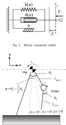
The following approach is based on the approximate for-mula of nonlinear muscle model, as shown in Fig. 2 [4].

F=u−kux−bux˙ (1)

In (1),F is total muscle force,uis muscle contraction unit,

xis the length of muscle which is defined as relative displace-ment from the natural lengthl0,kis the elastic coefficient, and

b is the viscous coefficient. Humans have antagonist muscles in each joint. For that reason, (1) is expressed as (2).

F= (uf−ue)−k(uf+ue)x−b(uf+ue) ˙x (2)

In (2), subscriptsfandedenote flexor and extensor muscle. In short, humans can adjustuf and ue to obtain the desired impedance characteristics.

Fig. 2. Muscle viscoelastic model.

Fig. 3. The influence of muscle length deviation in hamstrings.

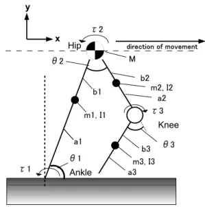
IV. THE STRAIGHT LINE RELATIONSHIP REPRESENTED BY HAMSTRINGS

According to the previous section, hamstrings (f3) espe-cially act in the latter part of the swing phase. Here, the authors describe why humans choose hamstrings instead of other redundant muscles. Output force of hamstrings, as shown in (3), can be derived from (2) and the length of moment arm

r which is the distance from a muscle’s line of action to the joint’s center of rotation.

F = u−ku(rhθh−rkθk)−bu(rhθ˙h−rkθ˙k) (3)

In (3), θ is angle of each joint defined by Fig. 3 and subscripts “h” and “k” denote “Hip” and “Knee”. Note thatθ

should be written in the displacement from the natural angle

θ0 which is defined by the natural length of muscle l0. This

time, however, the natural angle is set to zero for convenience. Here, the moment arm lengthrof hamstrings is focused. In case of Rectus femoris (e3), both side of the length of moment arm rh andrk is almost the same [8]. By contrast, in case of hamstrings (f3), the length of moment arm of hip is about twice as long as that of knee. The length of moment arm is generally vary with angle, however this relationship is almost satisfied in the swing phase [11].

If this relationship is adopted, the ratio of moment arm is

rh : rk = 2 : 1 in hamstrings. The joint torque of hip (Th) and knee (Tk) are described as (5) and (6).

F = u−kur(θh− 1 2θk)−bur( ˙θh− 1 2θ˙k) (4) Th = −r{u−kur(θh− 1 2θk)−bur( ˙θh− 1 2θ˙k)} (5) Tk = 1 2r{u−kur(θh− 1 2θk)−bur( ˙θh− 1 2θ˙k)} (6)

It is reasonable that muscle force effects hip joint stronger than knee joint because the lower part of a leg can be moved easily.

If the length of each link is the same as humans, φ =

θh−

1

2θk can be expressed as the straight line which connects

hip joint and knee joint. As shown in Fig. 3, this relationship looks like a simplified compasses model.∆x=r∆φdenotes deviation of hamstrings length from the natural length l0.

Given that the value of ∆x becomes large, feedback terms described in (5) and (6) also increase in order to reduce deviations.

Thus, this relationship implies that humans use hamstrings to employ the straight line relationship between hip and knee joint.

V. MATHEMATICAL EXAMINATION OF MUSCLE ACTIVATION PATTERNS

It is necessary to incorporate antagonistic activation to set the landing position. From (2), it can be balanced(uf −ue) withk(uf+ue)xat an equilibrium point. For that reason,uf andue should be adjusted to set given point.

For example, antagonistic muscles work in the plane surface without any disturbance [4] [5]. Joint torque can be expressed as (7). T =r(uf−ue)−kr 2 (uf+ue)θ−br 2 (uf+ue) ˙θ (7) In steady-state condition,θ˙andθ¨become zero. Hence,θis given by (8).

θ= uf−ue

kr(uf +ue)

(8) That is, the ratio of uf and ue defines the angle of equilibrium point.

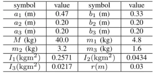
According to the previous section, humans do not use all their muscles simultaneously. Let us suppose the case (f3), (e1), and (e2) muscles act antagonistically. Here, a biped model shown in Fig. 4 is used.

A. Muscle activation model in the swing phase

At first, the non-linear equation of the biped walking model is taken into account, especially gravity effects.di consisting of non-linear equation of motion and disturbance is introduced for the moment. In steady-state condition,θ˙2,θ¨2,θ˙3, and θ¨3

are set to zero. Hence, major components ofdiare interference term of θ¨1 and gravity term. In conventional robots, precise

position tracking can be achieved by suppressing the effects ofdi. On the other hand, passivity based robots achieve high

Fig. 4. The biped walking model.

energy efficiency by employing the effects ofdi. The authors have emphasized that humans have both advantages. It is shown in following analysis.

The length of moment arm r, elastic coefficient k, and viscous coefficientbfor each muscle are regarded as the same value for simplicity. Most important characteristics are that bi-articular muscle (f3) acts two adjacent joints with different length of moment arm. In case of mono-articular muscles, this difference will be corporated into muscle contraction unitsui. If (f3), (e1), and (e2) muscles act antagonistically, joint torques are described in (9) and (10).

T2 = (ru2−ru23)−r 2 ku2θ2−r 2 ku23(θ2− 1 2θ3) − r2bu2θ˙2−r 2 bu23( ˙θ2− 1 2θ˙3)+d2 (9) T3 = ( 1 2ru23−ru3)−r 2 ku3θ3+ 1 2r 2 ku23(θ2− 1 2θ3) − r2bu3θ˙3+ 1 2r 2 bu23( ˙θ2− 1 2θ˙3)+d3 (10)

In (9) and (10), u23 is the muscle contraction unit of

hamstrings (f3), u2 is that of hip extensor muscles (e1), and

u3 is that of knee extensor muscles (e2).

The equilibrium point in steady-state condition is expressed as (11) and (12). θ2 = {(u3+ 1 4u23)D2+ 1 2u23D3}+{(u3+ 1 4u23) d2 r+ 1 2u23 d3 r} rk{(u3+ 1 4u23)u2+ 1 2u23(2u3)} (11) θ3 = {1 2u23D2+S2D3}+{ 1 2u23 d2 r +S2d_r3} rk{1 2u23( 1 2u2)+S2u3} (12) In (11) and (12), D2 = u2−u23, S2 = u2+u23, D3 = 1 2u23−u3, S3= 1

2u23+u3. In this case, the equilibrium point

is set by antagonistic muscles in arbitrary. The effects fromdi can be suppressed if muscle contraction units ui increase. It is like a exerting full strength of human’s motion.

TABLE I

THE MATH VARIABLES IN A BIPED WALKING MODEL FOR A CASE STUDY. symbol value symbol value

a1 (m) 0.47 b1(m) 0.33 a2 (m) 0.20 b2(m) 0.20 a3 (m) 0.20 b3(m) 0.20 M (kg) 40.0 m1 (kg) 4.8 m2 (kg) 3.2 m3 (kg) 1.6 I1(kgm2 ) 0.2571 I2(kgm2 ) 0.0434 I3(kgm2 ) 0.0217 r(m) 0.03

There are two equations (11) and (12) compared with three variables, therefore α = u2

u23, β =

u3

u23 are given for replacement, as shown in (13) and (14).

θ2 = (β+1 4)(α−1 + 1 u23 d2 r) + 1 2( 1 2−β+ 1 u23 d3 r) rk(αβ+1 4α+β) (13) θ3 = 1 2(α−1 + 1 u23 d2 r) + (α+ 1)( 1 2−β+ 1 u23 d3 r) rk(αβ+1 4α+β) (14) Here, θ∗

2 and θ∗3 are used as reference equilibrium points.

On the assumption thatu23has larger value, (13) and (14) can

be expressed as (15) and (16) usingΘi=rkθi∗.

α= 1 + Θ2− 1 2Θ3 1−Θ2 (15) β= 1 + Θ2− 1 2Θ3 2(1 + Θ3) (16)

αandβ can be uniquely specified if reference equilibrium points are given.u23 is freely chosen as a coefficient of total

muscle intensity to suppress the effects ofdi.

According to human walking, the muscle contraction inten-sity of hamstringsu23 gradually increases during the end of

the swing phase. If the effects ofdi become larger, the swing leg is practically moved by passive dynamics with low actuator torques. If the effects ofdi become smaller, the swing leg is moved by actuator torques with precise control. It means that humans can switch the control mode between “passive” and “active” gradually by usingu23.

VI. PARAMETER DETERMINATION FOR THE SIMULATION

In this section, actual muscle values are estimated for the simulation. The biped walking model is shown in Fig. 4 and Table I. The simulation was conducted in the initial posture

θ1 = 110 deg,θ2 = -30 deg,θ3 = 15 deg. MATLAB/simulink

have been employed for the simulation. The details of walking model such as an upper limb and feet are removed for simplicity.

As mentioned above, humans do not have the landing point consciously and there is no accurate control in the first part of the swing phase. For that reason, the hip joint torque is simply given to swing the leg in that time. For example, T2 =kθ˙1

which is proportional toθ˙1with low pass filter to smooth the

input torque. Besides, the stance leg illustrated in Fig. 4 is not actuated. It is driven by initial velocity θ˙1 and passive

dynamics.

Fig. 5. Block diagram of the proposed method. (f(α, β)denotes the ratio of muscle contraction force calculated by (15) and (16).)

The block diagram of the proposed method is shown in Fig. 5. Reference values are muscle contraction force of hamstrings

u23and landing angle of hamstrings(θ2− 1

2θ3)∗. According to

a landing posture of stable walking of humans, the knee angle

θ∗

3 is always extended. For this reason, the reference value of

θ∗

3 is set to the fixed valueθ3∗=−60deg. It means thatθ∗2 is

needed to set the landing point, but it is more natural to think the direction of straight line characteristics(θ2−

1 2θ3)∗.

A. Natural length l0 and viscoelastic coefficientsk, andb

Here, the natural angleθn is defined as the joint angle when the muscle length is naturall0. It is the intermediary position

of joint moving range in general, θ2n = 55 rad and θ3n = 65 rad. The authors have considered how θn effects to the walking motion.

Let us suppose that the target landing position is given asθ

=pin Fig. 4. It means the reference value is given byθ∗ _=p

-θn. If the natural angleθn changes, it is equivalent to change the reference angleθ∗_{. From (15) and (16), the ratio of muscle}

contractionα,βis varied byθ∗_{. When the value ofθ}∗

2becomes

large orθ∗_{3becomes small,αandβalso become large. In other}

words, the reference straight line angle(θ2− 1

2θ3)∗ is stepped

forward, the intensity of muscle contraction becomes stronger simultaneously. This is an advantage of considering the natural angle because the effect of gravity term is getting higher together with the value of(θ2−

1

2θ3)∗ that being said gravity

effect can be suppressed by stronger muscle contraction force automatically.

Viscoelastic coefficients k andb have been also estimated. From (2), real viscoelasticity of joints includes summation of antagonistic muscle contraction units. For that reason, it is difficult to measure the actual value of viscoelastic coefficients. However, the maximum value ofkis limited on the condition thatuimust be positive in (13) and (14). As a result,kshould be smaller than 30 N/m. In addition, the ratio of elasticity and viscosity is not influenced by muscle contraction units. For that reason,bcan be estimated byk.k= 10N/m andb= 1.3

Ns/m are used in this simulation.

B. Muscle contraction force of hamstringsu23

From human’s EMG pattern,u23 is proportional to time. It

means that effective viscoelastic coefficientsk′ _=ku

iandb′ =

buiwill be larger in order to change transient characteristics. If

u23 is increased proportionally, transient characteristics of θi also change under-damped to over-damped because effective

-1 -0.5 0 0.5 1 -0.5 0 0.5 1 x (m) y (m)

(a) stick diagram

0 0.5 1 -100 -50 0 50 100 150 Time (s)

Position error (deg)

θ₂ θ₃ θ₂ - 0.5θ₃

(b) position errors Fig. 6. Stick diagram and angle errors in case (I).

-1 -0.5 0 0.5 1 -0.5 0 0.5 1 x (m) y (m)

(a) stick diagram

0 0.5 1 -100 -50 0 50 100 150 Time (s)

Position error (deg)

θ₂ θ₃ θ₂ - 0.5θ

3

(b) position errors Fig. 7. Stick diagram and angle errors in case (II).

ofdi can be suppressed gradually, therefore u23 changes the

mode “passive” to “active” as mentioned above sections. Time variableu23 is approximated, as shown in (17).

u23=a(t−t0) (17)

In (17), a is the coefficient of intensity, t is time and

t0 is initial time. In following simulation, the authors have

determineda= 1.0×104

andt0= 0.2sec (about the middle

of the swing phase).

VII. NUMERICAL STUDY FOR EVALUATION OF PROPOSED METHOD

A. Followability of the reference position

Generally, the most efficient walking speed is about v = 1.0 - 1.5 m/s [12]. Here, the walking speed is given byv = 1.0 m/s for each pattern. In the simulation, the authors have considered in the following three cases.

(I) Reference value is set to (θ∗

2−

1

2θ∗3) = 30 deg. (A stick

diagram and position errors are illustrated in Fig. 6.) (II) Reference value is set to (θ∗

2−

1

2θ∗3)= 45 deg. (A stick

diagram and position errors are illustrated in Fig. 7.) (III) Reference value is set to(θ∗

2−

1

2θ∗3)= 15 deg. (A stick

diagram and position errors are illustrated in Fig. 8.)

As a result, position errors were nearly zero in all patterns. Therefore, the effects ofdi have been suppressed sufficiently.

B. Robustness under variable walking speedsv

Here, walking speedv is increased to v= 1.2 m/s. (IV) Reference value is set to(θ∗

2−

1

2θ∗3) = 45 deg, position

errors are illustrated in Fig. 9(a).

-1 -0.5 0 0.5 1 -0.5 0 0.5 1 x (m) y (m)

(a) stick diagram

0 0.5 1 -100 -50 0 50 100 150 Time (s)

Position error (deg)

θ₂ θ₃ θ₂ - 0.5θ₃

(b) position errors Fig. 8. Stick diagram and angle errors in case (III).

0 0.5 1 -100 -50 0 50 100 150 Time (s)

Position error (deg)

θ₂ θ₃ θ₂ - 0.5θ₃

(a) case (IV)

0 0.5 1 -100 -50 0 50 100 150 Time (s)

Position error (deg)

θ₂ θ₃ θ₂ - 0.5θ₃

(b) case (V) Fig. 9. Position errors whenv= 1.2 m/s.

(V) Reference value is set to (θ∗

2−

1

2θ3∗) = 15deg, position

errors are illustrated in Fig. 9(b).

In the case of (V), position errors are left to some extent. This is because there is not enough settling time and the swing leg collide to the ground before errors are settled. For this reason, it is necessary to set the landing point to a distant place when walking speed is increased. However, it is same as the case of human walking. If humans walk more high speed, walking step needs to be enlarged [12].

As a result, there are some constraint on walking speed and walking step. It is necessary to change the muscle contraction ratio αandβ to move the landing point farther.

C. Energy efficiency

The proposed control method is evaluated through compari-son with conventional control method. In conventional method, joint angles θ2 andθ3 are set to the reference angle by PD

controller. In order to evaluate under the same condition, PD gain is given by effective viscoelastic values in steady-state condition in case (I). Simulation conditions are the same as case (I) except for the control methods.

Position errors are illustrated in Fig. 10. Position errors are reduced quickly in the conventional method. However, passivity is sacrificed and steady-state errors are almost the same level as the proposed method. For that reason, there is no practical difference between them.

Input torques in the proposed and conventional methods are illustrated in Fig. 11. Comparing with the conventional method, peak torques are decreased in the proposed method, it is useful for reducing actuator size.

In addition, evaluation values of total energy consumption (=R |τ ω|dt) are illustrated in Fig. 12. Total energy

consump-0 0.5 1 -100 -50 0 50 100 150 Time (s)

Position error (deg)

θ₂ θ₃ θ₂ - 0.5θ₃

(a) the proposed method

0 0.5 1 -100 -50 0 50 100 150 Time (s)

Position error (deg)

θ₂ θ₃

(b) the conventional method Fig. 10. Position errors in the proposed and conventional methods.

0 0.5 1 -30 -20 -10 0 10 20 30 Time (s) Input torque (Nm) T hip T_knee

(a) the proposed method

0 0.5 1 -30 -20 -10 0 10 20 30 Time (s) Input torque (Nm) T hip T_knee

(b) the conventional method Fig. 11. Input actuator torques in the proposed and conventional methods.

tion in the proposed method is about 50% less than that in a conventional one.

Therefore, it has been cleared that landing position control with high energy efficiency can be achieved by the proposed method.

VIII. CONCLUSION

The authors have proposed a swing leg control method based on biological mechanisms and evaluated in advantages of better energy efficiency. Structure and patterns of muscle activation in biological legs were taken into account. A typical pattern of muscle activation has been observed from EMG waveforms, which implies the hamstrings play a major role in the motion in the swing phase.

Biological structure of lower limb and antagonistic muscles are significant in the muscle-based control for simplifying activation patterns. The proposed control method is based on the length and muscle contraction intensity of hamstrings. The length of hamstrings contributes to the intuitive design of the landing position with the straight line relationship. The muscle contraction intensity of hamstrings also contributes to the variation of the leg viscoelasticity. A repeatable and stable biped walking motion is possible by using passive dynamics according to the proposed control method.

A case study has been numerically calculated to verify the expected advantages of the proposed method, i.e, high energy efficiency and landing position control assuming dimensions and structure identical to a human body. As a result, energy consumption of the proposed method could be reduced by 50% compared with that in a conventional one.

The numerical results have suggested the following prob-lems to be improved in further studies. The proposed control

0 0.5 1 0 5 10 15 20 Time (s) Total power (W) T_hip T knee

(a) the proposed method

0 0.5 1 0 5 10 15 20 Time (s) Total power (W) T_hip T knee

(b) the conventional method Fig. 12. Evaluation values of total energy consumption in the proposed and conventional methods.

method shall be applied to an experimental bench. The pro-posed activation pattern is valid just in slower walking motion. The EMG measurement shows different, more complicated activation patterns for faster motions. Therefore, it will be difficult to determine parameters because of redundancy of muscles. In addition, muscle activation patterns in the stance phase and touch-down phase are very important from the point of view of energy saving walking. The proposed method should be expanded for practical use.

REFERENCES

[1] M. Kumamoto, “Evolution of motion control, revolution in humanoid robots,” Tokyo denki university press, 2006.

[2] V. Salvucci, Y. Kimura, S. Oh, and Y. Hori, “Force maximization of biarticularly actuated manipulators using infinity norm,” IEEE/ASME Transactions on Mechatronics, 2012.

[3] N. Hogan, “Adaptive control of mechanical impedance by coactivation of antagonist muscles,” IEEE Transactions on automatic control, Vol. AC-29, No. 8, 1984.

[4] K. Ito, and T. Tsuji, “The bilinear characteristics of muscle skeletomotor system and the application to prosthesis control,” The Transactions of Electrical Engineers of Japan 105-C, No.10, pp. 201-206, 1985. [5] K. Yoshida, T. Uchida, and Y. Hori, “Novel FF Control algorithm of

robot arm based on bi-articular muscle principle emulation of muscular viscoelasticity for disturbance suppression and path tracking,” Proc. of Annual Conference of the IEEE Industrial Electronics Society, pp. 310-315, 2007.

[6] P. Kormushev, B. Ugurlu, S. Calinon, N. G. Tsagarakis, and D. Caldwell, “Bipedal walking energy minimization by reinforcement learning with evolving policy parameterization,” Proc. of International Conference on Intelligent Robots and System, San Francisco, US, pp. 318-324, 2011. [7] D. P. Ferris, M. Louie, and C. T. Farley, “Running in the real world:

Adjusting leg stiffness for different surfaces,” Proc. of Royal Society London, vol. 265, pp. 989-993, 1998.

[8] Irving P. Herman, “Physics of the human body,” Springer, 2007. [9] E. A. Andersson, J. Nilsson, and A. Thorstensson, “Intramuscular EMG

from the hip flexor muscles during human locomotion,” Acta Physiol Scand, 161, pp. 361-370, 1997.

[10] H.J.A. van Hedel, L. Tomatis, and R. Muller, “Modulation of leg muscle activity and gait kinematics by walking speed and bodyweight unloading,” Gait Posture 24, 35-45, 2006.

[11] A. S. Arnold, S. Salinas, D. J. Asakawa, and S. L. Delp, “Accuracy of muscle moment arms estimated form MRI-based musculoskeletal models of the lower extremity,” Computer Assisted Surgery, Vol. 5, pp. 108-119, 2000.

[12] Y. Goto, K. Matsushita, K. Honma, A. Tsujino, and T. Okamoto, “Electromyographic study of walking pattern in relation to speed,” Annals of physical education, No.13, pp. 39-52, 1978.