ABSTRACT
The objective of this study is to empirically examine the dynamic causal relationship between oil price and economic growth in Kenya during the period from 1980 to 2015. In an effort to address the omission-of-variable bias, a trivariate Granger-causality framework that incorporates oil consumption as an intermittent variable between oil prices and economic growth – is employed. Using the newly developed autoregressive distributed lag (ARDL) bounds testing approach to cointegration and the Error-Correction Model-based Granger-causality framework, the results of the study reveal that there is distinct unidirectional Granger-causality flowing from economic growth to oil price in the study country. These results are found to apply both in the short run and in the long run. Thus, it can be concluded that in Kenya, it is the real sector that pushes oil prices up. Further, it is possible to predict oil price changes in Kenya – given the changes in economic growth.
1. Introduction
The quest to establish forces driving economic growth has left economists and policy makers digging deeper into various relationships between economic growth and other macroeconomic variables, energy included.
The relationship between energy and economic growth has attracted a proliferation of empirical studies in recent years, from both the impact and the causality angles alike [1-7]. However, studies particularly on energy prices and economic growth have not only been scanty but they have also been biased towards the impact of energy prices on economic growth – leaving the causality between economic growth and energy prices in general and oil prices in particular little explored [8,9].
Of the scanty studies on the latter, more than half have focused on the developed countries, developing Asian and Latin American countries, as well as selected oil producing countries. As a result, most African countries in general, and Kenya, in particular, are left with little or no coverage, it is these often forgotten
African countries that are, in most cases, hard hit by the oil price shocks [see 9]. In addition, the available studies on the causality between oil prices and economic growth have been far from being conclusive [4, 5, 10].
On the empirical front, studies on the causality between oil prices and economic growth can be conveniently grouped into four categories. The first group consists of studies that found Granger-causality to flow from oil prices to economic growth (see 11–13); while the second group found the flow to be from economic growth to oil prices [see, among others, 3, 14]. The third group is of studies that found the feedback hypothesis to be predominant [see among others, 4, 15, 16], while the fourth group constitutes studies that are consistent with the neutrality hypothesis (see 17–19).
Moreover, some previous studies on this subject have been found to suffer from two major weaknesses. Firstly, some of these studies have mainly used a bivariate causality test to examine this linkage; hence, they are prone to suffer from the omission-of-variable bias [see also 15, 20]. Secondly, some of these studies have
Oil price and economic growth in Kenya: A trivariate simulation
Nicholas Mbaya Odhiambo and Sheilla Nyasha
1Department of Economics, University of South Africa, P.O Box 392, UNISA, 0003, Pretoria, South Africa
Keywords:
Kenya, Oil prices, Energy consumption; Economic growth, Granger-causality; JEL Classification Code: O40, Q43;
URL:
mainly used the cross-sectional data to examine the causal relationship between oil prices and economic growth. This, unfortunately, does not address the country-specific effects.
Against this backdrop, the objective of this study is to empirically examine the dynamic causal relationship between oil prices and economic growth in Kenya using the newly developed ARDL-bounds-testing approach. By incorporating oil consumption in the bivariate model between oil prices and economic growth, a simple trivariate-causality model between oil prices, oil consumption and economic growth is examined. Contrary to the results of some previous studies, our results show that there is a distinct unidirectional causal flow from oil price to economic growth in Kenya.
The study is expected to contribute to the body of knowledge in more ways than one. The results of this study may guide authorities in Kenya on polices related to oil prices and economic growth and how best they can stimulate the real sector without fearing changes in oil price levels. Another benefit of the study comes from the methodology utilised, that provides country-specific, hence reliable, results. In addition, the study will add to the scanty literature available on the causality between oil price and economic growth.
The rest of the paper is organised as follows: Section two covers the dynamics of oil prices and economic growth in Kenya; while Section 3 reviews the literature. Section 4 presents the methodology used in the study, and Section 5 presents and analyses the results. Section 6 concludes the study.
2. Oil price increases and economic growth in Kenya
According to Omagwa et al. [21], the pricing of oil products in Kenya is often controlled by the relevant government department, making it a complex process. In 2016, according to the Kenya National Bureau of Statistics [22], the average crude oil price increased 20.3% compared to February prices of the same year. In the same period, the Brent oil price increased by $5.9 per barrel, reaching $39.07 per barrel. Historically, crude oil prices reached a maximum of $132.83 per barrel in July 2008, while record low prices of $1.17 per barrel were recorded in February 1946 [22].
A number of oil shocks have been experienced during the last +/- 50 years. Most of these oil shocks have been somewhat linked to the disruption of oil production in
the Middle East due to conflicts [8]. According to Hamilton [8], these conflicts include:
i) The closure of the Suez Canal following the conflict between Egypt, Israel, Britain, and France in October 1956
ii) The oil embargo implemented by the Arab members of OPEC following the Arab-Israeli War in October 1973
iii) The Iranian revolution beginning in November 1978
iv) The first Persian Gulf war beginning in August 1990.
Besides the oil shock, there are other events that were linked to the disruption of oil supply; and these were:
i) the combined effects of the second Persian Gulf War and strikes in Venezuela beginning in December 2002
ii) the Libyan revolution in February 2011.
Furthermore, oil price increases were part of the world energy landscape. The notable historical factors that have led to the oil price increases include:
i) the economic recovery from the East Asian Crisis in 1997
ii) the dislocations associated with post-World War II growth in 1947
iii) the Korean conflict in 1952-53.
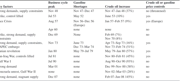
Table 1 presents a summary of events that significantly affected the post-independence Kenya.
On the economic growth front, Kenya’s economic growth has been significantly fluctuating since the 1970s. During the early years of independence, Kenya achieved commendable economic growth compared to other SSA countries. Between 1975 and 1985, the average annual percentage growth in GDP was 4.1% [23]. During the period 1985 to 1989, the average growth in GDP increased dramatically to 5.7% [23]. However, in 1991 the percentage change in GDP declined to 1.4%. In 1992, Kenya recorded a historic low GDP growth rate of about -0.8% – the lowest since independence. However, between 1993 and 1995, the GDP growth increased considerably. The GDP growth rate increased from about -0.8% in 1992 to 0.4% in 1993, before further increasing to 2.6% in 1994 [23]. By 1995 the GDP growth rate had reached 4.4%. But this high growth rate did not last for long. The GDP growth rate declined again systematically from 4.1% in 1996 to 0.5% in 1997 but bounced back to 3.3% in 1998. Just before the 2007 global financial crisis (GFC), Kenya’s growth rate was above 6%. Although the country was
into higher prices for consumer goods. This, in turn, lowers the consumption demand, which eventually leads to a contraction in real output [25]. However, according to supply-side effect, a rise in oil prices leads to higher production costs, which force producers to cut back their output – thereby lowering the country’s aggregate output [25].
While a number of studies have been conducted on the relationship between energy consumption and economic growth, the same cannot be said regarding the studies on the relationship between oil prices and economic growth – the latter are scanty.
The empirical literature has four categories in which the energy-growth causality outcomes can be grouped – the growth hypothesis, the conservation hypothesis, the feedback hypothesis, and the neutrality hypothesis [see 4, 5, 10]. Although the empirical literature on the causal relationship between oil prices and economic growth is still limited, each of the four categories established by empirical literature, regarding the possible causality outcomes, has found support – pointing to the conclusion that the causality results on the subject of study are mixed and inconsistent.
Most studies support the growth hypothesis and argue that it is energy consumption that Granger-causes economic growth [see 11– 13, 18, 26 – 33, among others]. There is, however, another strand that supports the conservation hypothesis and argues that it is the growth
negatively affected by the GFC, leading to faltering of economic activity – recording a growth rate of 0.2% in 2008 – it quickly recovered. By 2010, growth rate in Kenya was 8.4% [23].
From 2014 to 2016, economic growth averaged 5.6%, while in 2016 alone it was at 5.8%, placing Kenya as one of the fastest growing economies in SSA. According to the World Bank [24], a stable macroeconomic environment, low oil prices, rebound in tourism, strong remittance inflows and a government-led infrastructure development initiative were the key drivers of the high growth rate. However, GDP growth is expected to decelerate to 5.5% in 2017 as a result of the on-going drought and weak credit growth. The World Bank [24] projects Kenya’s GDP growth rate to rebound to 5.8% and 6.1% in 2018 and 2019, respectively, on the hopes of the completion of on-going infrastructure projects, a boom in tourism, resolution of slow credit growth and the strengthening of the global economy.
3. Literature review
On the theoretical front, an increase in oil prices is expected to have two effects – the demand-side effect and the supply-side effect [25, 26]. According to the demand-side effect, an increase in oil prices leads to an increase in transportation costs, which then translates
Table 1: Significant post-independence events in Kenya’s oil sector
Key factors
Business cycle peak
Gasoline
Shortages Crude oil increase
Crude oil or gasoline price controls
Strong demands, supply constraints Nov 48 Nov 47–Dec 47 Nov 47–Jan 48 (37%) no (threatened)
Strike, control lifted Jul 53 May 52 June 53 (10%) yes
Suez Crisis Aug 57 Nov 56–Dec 56
(Europe)
Jan 57–Feb 57 (9%) yes (Europe)
— Apr 60 none none no
Strike, strong demand, supply constraints
Dec 69 None Feb 69 (7%)
Nov 70 (8%)
no Strong demand, supply constraints,
OAPEC embargo Nov 73 June 73 Dec 73–Mar 74 Apr 73–Sep 73 (16%) Nov 73–Feb 74 (51%) yes
Iranian revolution Jan 80 May 79–Jul 79 May 79–Jan 80 (57%) yes
Iran-Iraq War, controls lifted Jul 81 none Nov 80–Feb 81 (45%) yes
Gulf War I Jul 90 none Aug 90–Oct 90 (93%) no
Strong demand Mar 01 none Dec 99–Nov 00 (38%) no
Venezuela unrest, Gulf War II none none Nov 02–Mar 03 (28%) no
Strong demand, stagnant supply Dec 07 none Feb 07–Jun 08 145%) no
Hanabusa [44] finds that there is a feedback relationship between the price of oil and economic growth in Japan. While examining the causal relationship between growth and oil price in small Pacific Island countries, Jayaraman and Choong [45] find that there is a unidirectional causal flow from oil price and international reserves to economic growth.
Although the bulk of the empirical studies support a negative relationship between oil price and economic growth, some recent studies have shown that this relationship may not be strictly negative for all countries. Prasad et al. [46], for example, while examining the relationship between oil prices and real GDP nexus in the Fiji Islands, find that an increase in the oil price has a positive, albeit inelastic, impact on real GDP. The authors conclude that although their finding is inconsistent with the bulk of the previous literature, it is not a surprising result for the Fiji Islands. Specifically, the authors argue that since the actual output in Fiji has been around 50% lower than its potential output, it has not reached a threshold level at which oil prices can negatively impact on output. Moreover, this finding, according to the authors, is consistent with the results from some emerging countries studied by the International Monetary Fund (IMF) [52].
4. Estimation techniques and empirical analysis
In order to empirically examine the causality between oil prices and economic growth in Kenya, the study utilises a trivariate Granger-causality model that incorporates oil consumption as an intermittent variable – so as to address the omission-of-variable bias associated with a bivariate model [see 53, 54).
To further distinguish itself from other previous studies, the study used an autoregressive distributed lag (ARDL) bounds-testing technique to examine this dynamic linkage between oil prices and economic growth in Kenya. The ARDL is a contemporary estimation technique that has been widely used of late because of numerous advantages it offers as compared to the its conventional counterparts – residual-based technique and the Full-Maximum Likelihood test [55]. With the ARDL approach, estimation can be carried out with variable integrated of order 0 or one or a mixture of both. Thus it does not restrict the variables to be integrated of the same order. In addition, even with endogenous regressors, the technique provides unbiased long-run estimates and valid of the real sector that drives the demand for energy
consumption [see, among others, 3, 14, 34 – 41]. Between these two extremes, there are studies that support bidirectional causality; hence they maintain that both energy consumption and economic growth Granger-cause each other. Studies that support this middle-ground view include Saidi et al. [4], Odhiambo [15], Paul and Bhattacharya [16], Yang [32], Glasure [42] and Masih and Masih [33]. Though uncommon, there are also studies that support the fourth view the neutrality hypothesis – that contends that there is no Granger-causality between oil consumption and economic growth [see 17–19, 25, 43].
Unlike the causal relationship between energy consumption and economic growth, the causal relationship between oil prices and economic growth has not been fully explored. Very few studies have fully examined the nexus between oil prices and economic growth. Some of the studies that have examined the relationship between oil prices and economic growth include Hanabusa [44], Jayaraman and Chooing [45], Prasad et al. [46], Rautava [47], Glasure and Lee [48], Kim and Willet [49] and Darrat and Gilley [50], among others.
Darrat and Gilley [50], for example, find that oil price shocks are not a major cause of US business cycles. In addition, the study finds that both oil prices and real output cause significant changes in oil consumption without feedback causal effects. While examining the relationship between oil price and economic growth in the Organisation for Economic Co-operation and Development (OECD) countries, Kim and Willet [49] find that there is a strong negative relationship between oil price and economic growth. Likewise, Glasure and Lee [48] find a significant negative relationship between oil price and economic growth for Korea. Using a vector autoregressive (VAR) model, Rautava [47] finds that Russia’s real GDP is negatively affected by oil price fluctuations.
Asafu-Adjaye [51] estimated the causal relationships between energy consumption and income in Asian developing countries – India, Indonesia, the Philippines and Thailand – cointegration and error-correction modelling techniques. The results indicated the presence of bidirectional Granger-causality between oil prices and economic growth in the case of Thailand and the Philippines
In an attempt to investigate the causal relationship between the price of oil and economic growth in Japan,
where:
y = per capita real gross domestic product OP = oil prices
OC = oil consumption
αo= respective constant; α1 – α3 = respective
short-run coefficients; α4 – α6 = respective long-run coefficients; ln = log operator; ∆ = difference operator; n = lag length; t = time period; and μit = white-noise error terms.
4.3. ECM-based Granger-causality model
Following Odhiambo [60] and based on the work of Pesaran and Shin [57] and Pesaran et al. [59], the ARDL-bounds testing approach adopted in this study can be expressed as:
t-statistics [56]. Unlike the conventional cointegration methods that estimate the long-run relationship using a system of equations, the ARDL technique uses only a single reduced form equation, making the estimation process simpler and easier without compromising the quality of results flowing from the analysis (55, 57]. Furthermore, with the ARDL estimation procedure, a sufficient number of lags are generated in order to obtain optimal lag length per variable via the data-generating process within a general-to-specific modelling framework. A list of the numerous advantages offered by the ARDL estimation procedure would not be complete without mention of its superior small-sample properties. This property enables the estimation of a model based on a limited dataset [3]. The ARDL is, thus, considered the most suitable analysis method for this study.
In order to overcome the traditional weaknesses associated with many conventional cointegration techniques, the study uses the recently introduced ARDL-bounds testing approach to examine the long-run relationship between oil prices and economic growth – within a trivatiate setting.
4.1 Data description
In this study, key variables are economic growth and oil prices. To this end, economic growth (y) is proxied by GDP per capita while oil price is proxied by the crude oil price. Oil consumption is the control variable and is proxied by energy use, as measured by kilograms of oil equivalent per capita. The choice of having this as a control variable was based on the theoretical empirical links it has with both key variables. On the one hand, oil consumption tends to drive economic growth [12, 58] while on the other hand, it may influence the price level of energy, inclusive of oil. The study used annual time-series data from 1980 to 2015 obtained from the World Bank DataBank [23]. 4.2. ECM-based cointegration model
Following Pesaran et al. [59], the cointegration equations associated with the trivariate Granger-causality models in this study are expressed as:
α α α α α α α µ = = = ∆ = + ∆ + ∆ + ∆ + + + +
∑
∑
∑
t n n i t i i t i i i n i t i t t i t t lny lny lnOP lnOC lny lnOP lnOC 0 1 - 2 -1 0 3 - 4 -1 5 -1 0 6 -1 1(1)
α α α α α α α µ = = = ∆ = + ∆ + ∆ + ∆ + + + +∑
∑
∑
t n n i t i i t i i i n i t i t i t t t lnOP lny lnOP lnOC lny lnOP lnOC 0 1 - 2 -0 1 3 - 4 -1 0 5 -1 6 -1 2 α α α α α α α µ = = = ∆ = + ∆ + ∆ + ∆ + + + +∑
∑
∑
t n n i t i i t i i i n i t i t i t t t lnOC lny lnOP lnOC lny lnOP lnOC 0 1 - 2 -0 0 3 - 4 -1 1 5 -1 6 -1 3(2)
(3)
α α α α δ µ = = = ∆ = + ∆ + ∆ + ∆ + +∑
∑
∑
t n n i t i i t i i i n i t i t t i lny lny lnOP lnOC ECM 0 1 - 2 -1 1 3 - -1 1 1 α α α α δ µ = = = ∆ = + ∆ + ∆ + ∆ + +∑
∑
∑
t n n i t i i t i i i n i t i t t i lnOP lny lnOP lnOC ECM 0 1 - 2 -1 1 3 - -1 2 1(4)
(5)
relationship between economic growth, oil prices and oil consumption – in a two-step process. The null hypothesis of no cointegration is tested against the alternative hypothesis of cointegration. First, the order of lags on the first differenced variables in the set of cointegration equations (1–3) is determined. The second step is the application of the bounds F-test to the same equations to determine the presence or absence of a long-run relationship between the variables under study.
If the calculated F-statistic is above the upper-bound level of the critical values provided by Pesaran et al. [59], the null hypothesis of no cointegration is rejected – and a conclusion that a long-run relationship exists, is reached. Should the calculated F-statistic be below the lower-bound level, the null hypothesis of no cointegration cannot be rejected. However, in the event that the calculated F-statistic falls within the upper- and the lower-bound levels, the results are deemed inconclusive. The results of the bounds F-test for cointegration are given in Table 2.
The cointegration results in Table 2 confirm the existence of one cointegrating vector; hence, Granger-causality can be tested.
5.3. ECM-based Granger-causality results
The short-run causality is established by the F-statistics on the explanatory variables derived from the Wald Test, while the long-run causality is determined by the negative sign and significance of the coefficient of the error-correction term. The results obtained from the estimation of Granger-causality model (equations 4–6) are presented in Table 3.
As reported in Table 3, the results of the Granger-causality model show that there is a distinct unidirectional causal flow from economic growth to oil prices in where ECM is the error-correction term and δ is its
coefficient.
5. Results and discussion
This section reports and analyses the results of the study and is subdivided into 3 parts. Section 5.1 covers stationarity while Section 5.2 is on cointegration; leaving Section 5.3 to cover the ECM-based Granger-causality. 5.1. Stationarity test
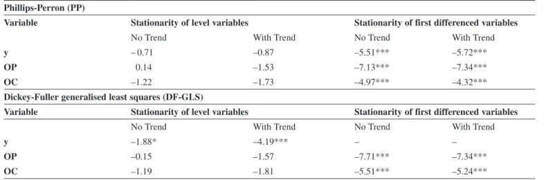
Although the ARDL-bounds testing approach does not require that the variables be tested for stationarity prior to analysis, the approach is not applicable if the variables are integrated of order two [I(2)] or higher. For this reason, stationarity tests were carried out using the Phillips-Perron (PP) and the Dickey-Fuller generalised least squares (DF-GLS) tests. These results are reported in Table 1.
The stationarity results confirmed that the variables where a mixture of those integrated of order zero and those integrated of order one – thereby fulfilling the ARDL stationarity condition.
5.2. Cointegration results
Having confirmed that all the variables included in the causality test are integrated of order not more than one, the next step is to test for the existence of a cointegration
Table 1: Stationarity results Phillips-Perron (PP)
Variable Stationarity of level variables Stationarity of first differenced variables
No Trend With Trend No Trend With Trend
y – 0.71 –0.87 –5.51*** –5.72***
OP 0.14 –1.53 –7.13*** –7.34***
OC –1.22 –1.73 –4.97*** –4.32***
Dickey-Fuller generalised least squares (DF-GLS)
Variable Stationarity of level variables Stationarity of first differenced variables
No Trend With Trend No Trend With Trend
y –1.88* –4.19*** – –
OP –0.15 –1.57 –7.71*** –7.34***
OC –1.19 –1.81 –5.51*** –5.24***
Note: * and *** denote stationarity at 10% and 1% significance level, respectively.
α α α α δ µ = = − = ∆ = + ∆ + ∆ + ∆ + +
∑
∑
∑
t n n i t i i t i i i n i t i t t i lnOC lny lnOP lnOC ECM 0 1 - 2 -1 1 3 - 1 3 1(6)
economic growth in Kenya during the period from 1980 to 2015. A trivariate Granger-causality model, which incorporated oil consumption as an intermittent variable, is used.
Although the energy consumption and economic growth nexus is gaining attention from researchers of late, little has been done on the specific relationship between oil prices and economic growth, in general, and in Kenya, in particular. In addition, a few of the studies available on the subject mostly suffer from a number of methodology-related weaknesses – such as the omission-of-variable bias emanating from the use of bivariate causality models, and use of cross-sectional methodologies that fail to incorporate country-specific issues.
Based on the ARDL bounds testing approach to cointegration and the ECM-based Granger-causality tests, results of this study reveal that there is distinct unidirectional Granger-causality flowing from economic growth to oil prices in the study country. These results are found to apply both in the short run an in the long run. Thus, it can be concluded that in Kenya, it is the real sector that pushes oil prices up. Further, it is possible to predict oil price changes in Kenya – given the changes in economic growth. However, the reverse – predicting the changes in economic growth given the changes in oil prices – is not possible. Hence, manipulation of the oil prices can be Kenya. These results apply irrespective of whether the
estimation is in the long run or in the short run.
The short-run results are confirmed by the F-statistics of economic growth (∆y) in the oil price function (∆OP) that is statistically significant – and the long-run results are supported by the error-correction term (ECMt-1) in the same function, that is both negative and statistically significant at 10% level. These results are consistent with the conservation hypothesis – one of the four hypotheses postulated in the energy-growth theoretical literature – that states that it is the increase in economic development that causes the demand for energy to increase. Thus, in this case, it is the growth of the real sector that pushes oil prices, implying that Kenyan consumers have the ability to thrive even when prices are high. These results are consistent with Shahbaz et al.
[14] and Odhiambo [15], among others.
The results further show that there is bidirectional causality between economic growth and oil consumption – but only in the short run – as firmed by the coefficients of oil consumption (∆OC) and economic growth (∆y) in the economic growth and oil consumption functions, respectively, that are statistically significant at 10% and 5% levels, respectively.
6. Conclusion
Table 2: Bounds F-test for cointegration
Dependent variable Function F-statistic Cointegration status
y F(y|OP, OC) 2.76 Not cointegrated
OP F(OP|y, OC) 5.03** Cointegrated
OC F(OC|y, OP) 0.46 Not cointegrated
Asymptotic critical values Pesaran et al. [59],
p.300 Table CI(iii) Case III
1% 5% 10%
I(0) I(1) I(0) I(1) I(0) I(1)
5.15 6.36 3.79 4.85 3.17 4.14
Note: ** statistical significance at 5% level
Table 3: Results of Granger-causality tests
F-statistics [probability] ECTt-1
[t-statistics] Dependent variable ∆yt ∆OPt ∆OCt ∆yt – 0.363 [0.551] 4.005* [0.054] – ∆OPt 3.294* [0.080] – 0.744 [0.978] -0.391* [-1.988] ∆OCt 6.497** [0.016] 0.002 [0.968] – –
[12] Odhiambo, N.M. Energy consumption and economic growth nexus in Tanzania: an ARDL bounds testing approach. Energy Policy 37(2) (2009a) 617-622. https://doi.org/10.1016/j. enpol.2008.09.077
[13] Narayan, P.K., Smyth, R. Energy consumption and real GDP in G7 countries: new evidence from panel cointegration with structural breaks. Energy Economics 30 (2008) 2331-2341. https://doi.org/10.1016/j.eneco.2007.10.006
[14] Shahbaz, M., Van Hoang, T.H., Mahalik, M.K., and Roubaud, D. Energy consumption: Financial development and economic growth in India: New evidence from a nonlinear and asymmetric analysis. Energy Economics, 63 (2017) 199-212. https://doi. org/10.1016/j.eneco.2017.01.023
[15] Odhiambo, N.M. Electricity consumption and economic growth in South Africa: a trivariate causality test. Energy Economics 31(5) (2009b) 635-640. http://dx.doi.org/10.1016/j. eneco.2009.01.005
[16] Paul, S., Bhattachrya, R.B. Causality between energy consumption and economic growth in India: a note on conflicting results. Energy Economics 26 (2004) 977-983. http://dx.doi.org/10.1016/j.eneco.2004.07.002
[17] Rahman, M.M., and Mamun, S.A.K. Energy use, international trade and economic growth nexus in Australia: New evidence from an extended growth model. Renewable and Sustainable Energy Reviews, 64 (2016) 806-816. https://doi.org/10.1016/j. rser.2016.06.039
[18] Cheng, B.S. Energy consumption and economic growth in Brazil, Mexico and Venezuela: a time series analysis. Applied Economics Letters 4 (1997) 671-674.
[19] Cheng, B.S. An investigation of cointegration and causality between energy consumption and economic growth. Journal of Energy and Development 21 (1995) 73-84.
[20] Odhiambo, N.M. Financial depth, savings and economic growth in Kenya: a dynamic causal relationship. Economic Modelling 25 (4) (2008) 704-713. https://doi.org/10.1016/j. econmod.2007.10.009
[21] Omagwa, J., Kihooto, E. and Reardon, G. Oil Retail Pricing and Price Controls: A Case of Oil Marketing Sector in Kenya. Journal of Economics and Sustainable Development, 8(2) (2017) 114-120. https://www.ku.ac.ke/schools/business/ images/stories/research/Oil%20Retail%20Pricing%20and%20 Price%20Controls%20Article-%20Online%20version.pdf [22] Kenya National Bureau of Statistics (KNBS). Economic
Survey 2018 (2018) https://s3-eu-west-1.amazonaws.com/s3. sourceafrica.net/documents/118312/Kenya-Economic-Survey-2018.pdf
[23] World Bank. World development indicators (2018a) [Online] Available from <http://databank.worldbank.org/data/databases. aspx> [Accessed 16 May 2018].
oil consumption that was found to have feedback effect on economic growth, but only in the short run.
References
[1] Ghalayini, L. The Interaction between Oil Price and Economic Growth. Middle Eastern Finance and Economics, 13 (2011) 128-141 http://www.eurojournals.com/MEFE.htm
[2] Blanchard, O.J., Galí, J. The macroeconomic effects of oil price shocks: Why are the 2000s so different from the 1970s? In International Dimensions of Monetary Policy; NBER Chapters; National Bureau of Economic Research, Inc.: Cambridge, MA, USA (2007) 373-421. RePEc:upf:upfgen:1045
[3] Odhiambo, N.M. Coal consumption and economic growth in South Africa: An empirical investigation. Energy & Environment, 27(2) (2016) 215-226. https://doi. org/10.1177/0958305X15627535
[4] Saidi, K., Rahman, M.M. and Amamri, M. The causal nexus between economic growth and energy consumption: New evidence from global panel of 53 countries. Sustainable Cities and Society, 33 (2017) 45-56. https://doi.org/10.1016/j. scs.2017.05.013
[5] Tiba, S. and Omri, A. Literature Survey on the Relationships between Energy, Environment and Economic Growth. Renewable and Sustainable Energy Reviews, 69 (2017) 1129-1146. https://doi.org/10.1016/j.rser.2016.09.113
[6] Frimpong, P.B., Antwi,A.O., Brew, S.E.Y. Effect of energy prices on economic growth in the ECOWAS sub-region: Investigating the channels using panel data. Journal of African Business 19(2) (2018) 227-243, HTTP://DX.DOI.ORG/ 10.1080/15228916.2017.1405706 [7] Nyasha, S., Gwenhure, Y., Odhiambo, N.M. Energy
consumption and economic growth in Ethiopia: A dynamic causal linkage. Energy & Environment forthcoming (2018) HTTP://DX.DOI.ORG/ 10.1177/0958305X18779574
[8] Hamilton, J.D. Oil prices, exhaustible resources, and economic growth. In Handbook on Energy and Climate Change, Edward Elgar Publishing (2013) 29-63.
[9] Gadea, M.D., Gómez-Loscos, A Montañés, A. Oil Price and Economic Growth: A Long Story? Econometrics 41(4) (2016) 1-28. HTTP://DX.DOI.ORG/10.3390/econometrics4040041 [10] Shahbaz, M., Zakaria, M., Shahzad, S.J.H. and Mahalik, M.K.
The energy consumption and economic growth nexus in top ten energy-consuming countries: Fresh evidence from using the quantile-on-quantile approach. Energy Economics, 56(C) (2018) 177-184. RePEc:pra:mprapa:84920
[11] Destek, M.A. Natural gas consumption and economic growth: Panel evidence from OECD countries. Energy, 114 (2016) 1007-1015. http://dx.doi.org/10.1016/j.energy.2016.08.076
[38] Cheng, B.S. Causality between energy consumption and economic growth in India: an application of cointegration and error-correction modeling. Indian Economic Review 34 (1) (1999) 39-49. https://www.jstor.org/stable/29794181
[39] Cheng, B.S., Lai, T.W. An investigation of cointegration and causality between energy consumption and economic activity in Taiwan. Energy Economics 19 (1997) 435-444. RePEc:eee:eneeco:v:19:y:1997:i:4:p:435-444
[40] Abosedra, S., Baghestani, H. New evidence on the causal relationship between United States energy consumption and gross national product. Journal of Energy Development 14 (1989) 285-292. https://www.jstor.org/stable/24807939 [41] Kraft, J., Kraft, A. On the relationship between energy and
GNP. Journal of Energy Development 3 (1978) 401-403. https://www.scirp.org/(S(i43dyn45teexjx455qlt3d2q))/ reference/ReferencesPapers.aspx?ReferenceID=98488
[42] Glasure, Y.U. Energy and national income in Korea: further evidence on the role of omitted variables. Energy Economics 24 (2002) 355-365. https://doi.org/10.1016/S0140-9883(02)00036-1
[43] Yu, E.S.H., Hwang, B.K. The relationship between energy and GNP: further results. Energy Economics 6 (1984) 186-1990. https://doi.org/10.1016/0140-9883(84)90015-X
[44] Hanabusa, K. Causality between the price of oil and economic growth in Japan. Energy Policy 37 (2009) 1953-1957. https://
doi.org/10.1016/j.enpol.2009.02.007
[45] Jayaraman, T.K., Choong, C. Growth and oil price: a study of causal relationships in small Pacific Island countries. Energy Policy 37 (2009) 2182-2189. http://dx.doi.org/10.1016/ jenpol.2009.01.025
[46] Prasad, A., Narayan, P.K., Narayan, J. Exploring the oil price and real GDP nexus for a small island economy, the Fiji Islands. Energy Policy 35 (2007) 6506 - 6523. https://doi. org/10.1016/j.enpol.2007.07.032
[47] Rautava, J. The role of oil prices and the real exchange rate in Russia’s economy – a cointegration approach. Journal of Comparative Economics 32 (2004) 315-327. https://doi. org/10.1016/j.jce.2004.02.006
[48] Glasure, Y.U., Lee, A.R. The Impact of oil prices on income and energy. International Advances in Economic Research 8 (2002) 148-154. https://link.springer.com/article/10.1007/ BF02295345
[49] Kim, S., Willett, T.D. Is the negative correlation between inflation and economic growth real? An analysis of the effect of the oil supply shocks. Applied Economics Letters 7 (2000) 141-147. https://doi.org/10.1080/135048500351681
[50] Darrat, A.F., Gilley, O.W. US oil consumption, oil prices, and the macroeconomy. Empirical Economics 21 (1996), 317-334 http://dx.doi.org/10.1007/BF01179861
[24] World Bank. Kenya Overview (2018b) [Online] Available from <http://www.worldbank.org/en/country/kenya/overview> [Accessed 16 May 2018].
[25] Akarca, A.T., Long, T.V. On the relationship between energy and GNP: a reexamination. Journal of Energy Development 5 (1980) 326-31.
[26] Altinay, G., Karagol, E. Electricity consumption and economic growth: evidence from Turkey. Energy Economics 27 (2005) 849-856. RePEc:eee:eneeco:v:27:y:2005:i:6:p:849-856 [27] Narayan, P.K., Prasad, A. Electricity consumption – real GDP
causality nexus: Evidence from a bootstrapped causality test for 30 OECD countries. Energy Policy 36 (2008) 910-918. https:// doi.org/10.1016/j.enpol.2007.10.017
[28] Narayan, P.K., Singh, B. The electricity consumption and GDP nexus for Fiji Islands. Energy Economics 29 (2007) 1141-1150. https://doi.org/10.1016/j.eneco.2006.05.018
[29] Wolde-Rufael, Y. Disaggregated energy consumption and GDP; the experience of Shanghai, 1952-99. Energy economics 26 (2004) 69-75. https://doi.org/10.1016/S0140-9883(03)00032-X [30] Shiu, A., Lam, P.L. Electricity consumption and economic
growth in China. Energy Policy 32 (2004) 47-54. https://doi. org/10.1016/S0301-4215(02)00250-1
[31] Chang, T., Fang, W., Wen, L. Energy consumption, employment, output, and temporal causality: evidence from Taiwan based on cointegration and error-correction modeling techniques. Applied Economics 33 (2001) 1045-1056.
[32] Yang, H.Y. A note on the causal relationship between energy and GDP in Taiwan. Energy Economics 22 (2000) 309-317. https://doi.org/10.1016/S0140-9883(99)00044-4
[33] Masih, A.M.M., Masih, R. On the causal relationship between energy consumption, real income prices: some new evidence from Asian NICs based on multivariate cointegration / vector error correction approach. Journal of Policy Modeling 19 (1997) 417-440. https://doi.org/10.1016/S0161-8938(96)00063-4 [34] Mozumder, P., Marathe, A. Causality relationship between
electricity consumption and GDP in Bangladesh. Energy Policy 35 (2007) 395-402. https://doi.org/10.1016/j.enpol.2005.11.033 [35] Hatemi-J, A., Irandoust, M. Energy consumption and eco-nomic growth in Sweden: a leveraged bootstrap approach (1965-2000). International Journal of Applied Econometrics and Quantitative Studies 2-4 (2005) 87-98.
RePEc:eaa:ijaeqs:v:2:y2005:i:4_6
[36] Narayan, P.K., Smyth, R. Electricity consumption, employment and real income in Australia: evidence from multivariate Granger causality tests. Energy Policy 33 (2005) 1109-1116. https://doi.org/10.1016/j.enpol.2003.11.010
[37] Gosh, S. Electricity consumption and economic growth in India. Energy Policy 30 (2002) 125-129. https://doi.org/10.1016/ S0301-4215(01)00078-7
Countries. Managing Global Transitions, 15(1) (2017) 81-101. RePEc:mgt:youmgt:v:15:y:2017:i:1:p:81-101
[57] Pesaran, M., Shin, Y. An autoregressive distributed lag modeling approach to cointegration analysis” in S. Strom, (ed) Econometrics and Economic Theory in the 20th Century: The Ragnar Frisch centennial Symposium, Cambidge University Press, Cambridge (1999).
[58] Apergis, N., Payne, J.E. A panel study of nuclear energy consumption and economic growth. Energy Economics 32 (2010) 545-549. http://dx.doi.org/10.1016/j.eneco.2009.09.015 [59] Pesaran, M., Shin, Y., Smith, R. Bounds testing approaches to
the analysis of level relationships. Journal of Applied Econometrics 16 (2001) 289-326. https://doi.org/10.1002/ jae.616
[60] Odhiambo, N.M. Energy Consumption, Prices and economic growth in three SSA countries: A comparative study. Energy Policy, 38 (2010) 2463-2469. https://doi.org/10.1016/j. enpol.2009.12.040
[51] Asafu-Adjaye, J. The relationship between energy consumption, energy prices and economic growth: time series evidence from Asian developing countries. Energy Economics, 22(6) (2000) 615-625. http://dx.doi.org/10.1016/S0140-9883(00)00050-5 [52] International Monetary Fund (IMF). The impact of high oil
prices on the global economy (2000) IMF, Washington, D.C. [53] Loizides, J. and Vamvoukas, G. Government expenditure and
economic growth: Evidence from trivariate causality testing. Journal of Applied Economics, 8(1) (2005) 125-152. https:// ageconsearch.umn.edu/bitstream/37515/2/loizides.pdf
[54] Nyasha, S. and Odhiambo, N.M. The Impact of Banks and Stock Market Development on Economic Growth in South Africa: An ARDL-Bounds Testing Approach. Contemporary Economics, 9(1) (2015) 93-108. https://papers.ssrn.com/sol3/ papers.cfm?abstract_id=2607432
[55] Duasa, J. Determinants of Malaysian trade balance: An ARDL bounds testing approach. Journal of Economic Cooperation, 28(3) (2007) 21-40. https://pdfs.semanticscholar. org/7f33/296edcf1ad9fa259d6053ee80ceab976e001.pdf [56] Nyasha, S. and Odhiambo, N.M. Are Banks and Stock Markets