Testing for the underlying dynamics of bank capital buffer and performance nexus

Testing for the underlying dynamics of bank capital buffer and 

performance nexus

Article (Accepted Version)

http://sro.sussex.ac.uk

This version is available from Sussex Research Online: http://sro.sussex.ac.uk/id/eprint/76177/

This document is made available in accordance with publisher policies and may differ from the published version or from the version of record. If you wish to cite this item you are advised to consult the publisher’s version. Please see the URL above for details on accessing the published version.

Copyright and reuse:

Sussex Research Online is a digital repository of the research output of the University.

Copyright and all moral rights to the version of the paper presented here belong to the individual author(s) and/or other copyright owners. To the extent reasonable and practicable, the material made available in SRO has been checked for eligibility before being made available.

Copies of full text items generally can be reproduced, displayed or performed and given to third parties in any format or medium for personal research or study, educational, or not-for-profit purposes without prior permission or charge, provided that the authors, title and full bibliographic details are credited, a hyperlink and/or URL is given for the original metadata page and the content is not changed in any way.

1 Testing for the underlying dynamics of bank capital buffer and performance

nexus.

Mamatzakis E.1 _{and A. Bagntasarian}2

February 2018

Abstract

This paper reveals the underlying dynamics between the capital buffer and bank performance in EU-27 countries. A dynamic panel analysis shows that capital buffer is significantly affected by bank performance and risk exposure. Remarkably, a threshold analysis identifies regime changes for the underlying relationships during the financial crisis of 2008. We find a positive relationship between the capital buffer and performance for banks that fall in the low performance regime, while a negative relationship is reported for the banks that belong to the high regime. Threshold results also show that buffer exerts a positive impact on bank performance. Although regulation reforms that aim to raise the capital requirements could improve bank performance and stability, these improvements are not homogeneous across banks.

Keywords: Capital buffer; Dynamic threshold; Performance; Bank default risk. JEL classification: G20; G21; G28

a_{School of Business, Management and Economics, Jubilee Building, University of Sussex,}

Falmer, BN1 9SL, UK, e-mail: [email protected],

b_{School of Business, Management and Economics, Jubilee Building, University of Sussex,}

2 1. Introduction

The financial crisis of 2008 shows that sudden changes in asset quality and value can quickly diminish bank capital, leaving banks with inadequate capital to deal with unexpected losses. As a result, capital buffer requirements have become an instrument of providing cushion during adverse economic conditions. In some respect, capital buffer is a macro-prudential tool that could prevent bank excessive risk-taking (Ayuso et al. 2004; Jokipii and Milne 2008). Under Basel III, banks need to maintain a mandatory capital buffer of 2.5 percent of common equity. In the case of violation of this minimum requirement, the Basel Committee would assert restrictions on dividends and remunerations. Furthermore, Basel Committee may also require a discretionary counter-cyclical buffer up to another 2.5 percent of capital during periods when funds are easy to borrow. The main aim of counter-cyclical buffer is to prevent market instability during periods of excessive credit growth by providing banks with extra capital (Krug et al. 2015). Banks also have an incentive to hold capital buffer in order to signal soundness and thereby, receive higher credit rating scores. In addition, banks may hold a capital buffer to avoid costs related to penalties and restrictions imposed by the regulators when the former violate minimum capital requirements (Buser et al. 1981; Jokipii and Milne 2011). Finally, there is a vast literature on examining the association between capital requirements and bank’s asset structure (Alali and Jaggi 2011; Chu et al. 2007; Furfine 2001; Pasiouras et al. 2006; Repullo and Suarez 2012; Rime, 2001; Shrieves and Dahl, 1992). Since regulators imply restrictions on banks to limit their risk exposure, it could be the case that banks with a higher risk exposure might maintain a

3 higher capital buffer (Baule 2014; Calomiris and Wilson 2004; Flannery and Rangan 2008; Jokipii and Milne 2008, 2011).

Despite the benefits of financial stability due to the adequate capital buffer, some literature argues that raising capital through capital markets is costly especially during economic downturns (Alfon et al. 2004; Ayuso et al. 2004; Berger and Bonaccorsi di Patti 2006). Banks might rely on their own profitability to build up a capital buffer (Shim 2013). To this day, there is not a clear consensus in the literature on the relationship between the capital buffer and bank performance. There are studies that provide evidence for a negative association between bank performance and capital buffer (Alfon et al. 2004; Ayuso et al. 2004; Berger and Bonaccorsi di Patti 2006; Jokipii and Milne 2008) suggesting that strong bank performance substitutes for capital as a cushion against unexpected losses. Another strand of literature (Berger 1995, Flannery and Rangan, 2008; Nier and Bauman 2006; Shim 2013) finds a positive relationship between performance and buffer indicating that an improvement in bank performance increases buffer.

Concerning the capital buffer and risk nexus, there are several empirical studies (Baule 2014; Calomiris and Wilson 2004; Flannery and Rangan 2008; Francis and Osborne 2012; Jokipii and Milne 2008; Shim 2013) testing whether increasing the risk taken by banks force them to maintain a higher capital buffer. The results show that there is a positive relationship between bank risk-taking and capital buffer, indicating that banks with a greater risk exposure choose to hold a higher capital buffer. Following previous literature (Ayuso et al. 2004; Jokipii and Milne 2008), we employ non-performing loans,

4 off-balance-sheet items and risk-weighted assets to account for bank risk exposure, while as a measure of bank default risk we include Altman’s Z-Score (Altman 1968). This paper contributes to the literature of the relationship between capital buffer, bank performance and risk in several ways. First of all, unlike previous studies, this paper employs a dynamic panel threshold analysis. Similarly to the conventional dynamic panel analysis, threshold methodology accounts for the dynamic nature of capital buffer and for the potential endogeneity of the explanatory variables. The main advantage of the threshold analysis over dynamic panel regressions is that it allows data itself to define the crisis years. Thus, threshold analysis identifies the presence of regime switches in the relationship between the capital buffer and other bank-specific variables. Specifically, we investigate the presence of regime switches for the relationship between a) capital buffer and performance as measured by bank efficiency and b) capital buffer and risk of default as measured by Altman’s Z-Score. Furthermore, we account for the inverse relationship between these variables. For this reason, we examine the impact of capital buffer on bank performance and Altman’s Z-Score using buffer as a threshold variable. Additionally, we opt for different measures of performance and risk to reveal all potential determinants of bank capital buffer. Finally, this study covers a period (2004 – 2013) that includes the crisis years and therefore, we take into account any differences due to the financial meltdown in 2007 – 2008 and the recovery thereafter. This study confirms prior research, suggesting that bank performance and risk have a strong impact on the capital buffer. However, this analysis shows that the impact of efficiency on buffer varies across banks. Estimated results demonstrate a strong positive impact of performance on the buffer for banks in the low performance regime,

5 while for the relatively better performing banks a further improvement in performance would reduce capital buffer. Furthermore, we show that capital buffer would reduce bank risk of default. We also perform a sensitivity analysis to account for any potential endogeneity and therefore, underlying causality, opting for a flexible panel VAR model. This model provides the response of bank capital buffer to shocks in efficiency and risk of default in the VAR.

The paper is organised as follows. Section 2 sets the hypotheses to be tested in the empirical section. Section 3 presents our data, whilst section 4 discusses the methodology. Next, section 5 reports regression results and the subsequent threshold analysis. Section 6 develops our sensitivity analysis employing Panel-VAR methodology and finally, section 7 concludes.

2. Hypotheses development

2.1.The dynamic adjustment hypothesis

Following previous literature (Ayuso et al. 2004; Guidara et al. 2013; Jokipii and Milne 2008, 2011; Stolz and Wedow 2011), we hypothesise that banks might need time to adjust their capital buffer. In the absence of adjustment costs in capital ratio, banks would not hold capital in excess of the minimum regulatory requirement (Stolz and Wedow 2011). As banks would adjust the capital buffer with some time lags, the capital buffer of the previous period should have a positive and statistically significant impact on the current capital buffer.

H1. Adjustment in bank capital would affect positively the capital buffer.

6 Past research (Alfon 2004; Ayuso et al. 2004; Guidara et al. 2013; Jokipii and Milne 2008; Nier and Baumann 2006; Rime 2001; Shim 2013) provides mixed results regarding the relationship between bank capital buffer and performance. Alfon (2004), Ayuso et al. (2004), Guidara et al. (2013) and Jokipii and Milne (2008) find a negative relationship between capital and ROE. Berger (1995), Flannery and Rangan (2008), Nier and Baumann (2006), Rime (2001) and Shim (2013) provide evidence of a positive relationship between bank profitability and capital buffer, indicating that more profitable banks hold a higher capital buffer. This strand of literature is in line with the pecking order theory, according to which banks prefer retained earnings as their main source of financing since external sources can be costly (Myers and Majluf 1984). In this study, beyond the accounting measures of bank performance such as return on equity (ROE), return on assets (ROA) and net interest margin (NIM), we also employ bank’s cost efficiency derived from the Stochastic Frontier Analysis (SFA). Although, there have been several studies about the link between total regulatory capital and efficiency, up till now the literature on the relationship between the capital buffer and efficiency has been rather inconclusive. In an early study, Kwan and Eisenbeis (1997) using quarterly data over the period 1986 – 1995 for 352 U.S. bank holding companies, examine the relationships among bank risk-taking, capital and efficiency. The authors document a positive relationship between inefficiency and capital providing evidence of regulatory pressure over underperforming banks to maintain more capital. Moreover, the authors show that better capitalized banks exhibit a higher level of efficiency than less capitalized banks.

7 Berger and Bonaccorsi di Patti (2006) find a negative relationship between regulatory capital and efficiency for U.S. banks over the period 1990 – 1995. Their results support the “efficient-risk hypothesis” which suggests that more efficient institutions would hold relatively low capital, since higher expected returns from the greater efficiency may substitute capital.

In line with these results, Altunbas et al. (2007) using a sample of European banks for the period 1992 – 2000, show that inefficient European banks tend to hold more capital and evolve in less risky activities.1 _{These results provide further support for the} regulatory pressure over underperforming banks to maintain more capital. However, Altunbas et al. (2007) argue that this relationship varies with the level of bank efficiency and across ownership types.

Arguably, the opposite relationship might also exist supporting the “franchise-value hypothesis” (Berger and Bonaccorsi di Patti 2006). According to the“franchise-value hypothesis”, more efficient institutions tend to maintain a relatively high capital to protect their franchise value and future income derived from high efficiency (Berger and Bonaccorsi di Patti 2006; Kwan and Eisenbeis 1997). This hypothesis could also be reinforced by the pecking order theory according to which banks will prefer to finance their capital needs internally, especially when the access to capital markets is difficult. Therefore, more efficient banks that are expected to be more profitable (Althanasoglou et al. 2008; Berger et al. 1997; Goddard et al. 2009; Oral and Yolalan 1990), may hold greater capital buffer.

8 Thus, since a further analysis is warranted to determine the relationship between capital buffer and bank performance, our second hypothesis is developed as follows:

H2. Bank performance enhances bank capital buffer.

2.3.Bank risk exposure hypothesis

During the last decade, regulators have emphasized the importance of capital requirements in order to mitigate risk-taking and enhance the financial stability of the banking industry. The implementation of higher capital requirements aims to create a direct link between banks’ capital and risk. It could be the case that banks with a greater risk exposure may have to maintain a higher level of capital (Nier and Baumann 2006). In line with this view, prior literature (Calomiris and Wilson 2004; Flannery and Rangan 2008; Jokipii and Milne 2008, 2011; Rime 2001; Shrieves and Dahl 1992) find a positive relationship between bank capital buffer and risk, indicating that banks with risky positions hold higher buffers. This strand of literature provides evidence supporting the “regulatory hypothesis” according to which regulators encourage banks with a higher risk exposure to hold a higher capital buffer. The reason is that banks that hold risky portfolios but do not maintain a higher buffer are more likely to end up with capital below the minimum requirement.

On the other hand, the “moral hazard hypothesis” proposes a negative relationship between capital and risk. According to this hypothesis, banks might exploit flat-rate deposit insurance schemes (Demirgüç-Kunt and Kane 2002).2 _{It could be the case that}

2 _{Consistent with this theory, Jacques and Nigro (1997) document a negative association between changes} in capital and risk during the first year of the risk-based standards. The authors note that such a result might be due to the methodological issues in the risk-based guidelines where the weights assigned to assets classes might not reflect the true risk.

9 banks with greater risk exposure may hold lower capital buffer if all depositors are insured.3

As the literature it is not conclusive, we test the following hypothesis: H3. Risk exerts a positive impact on bank capital buffer.

3. Data and variables

We use an unbalanced bank-level panel data that includes saving and commercial banks from EU-27 countries over the period 2004 – 2013 on annual basis.4 _{Our analysis uses} 1,017 banks and a total of 3,788 observations. The primary source of our data is the Bankscope database by Bureau van Dijk, while we obtain macroeconomic data from the World Bank.

3.1.Measuring bank capital buffer

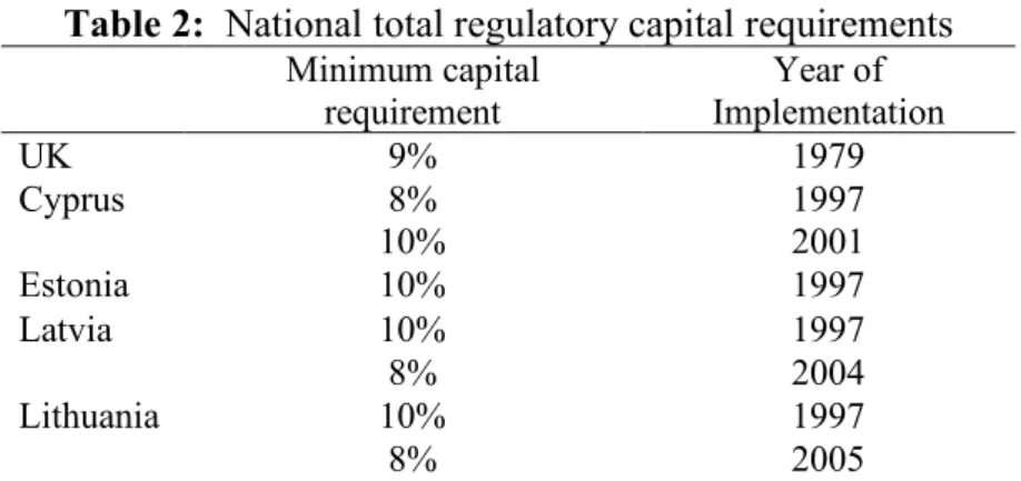
We define the capital buffer as the amount of capital banks hold in excess of the minimum requirement (Ayuso et al. 2004; Guidara et al. 2013; Jokipii and Milne 2008, 2011). Table 1 and Figure 1 present the variability of total regulatory capital (Tier 1 plus Tier 2 over Risk Weighted Assets) across country and over time respectively. Following Jokipii and Milne (2008), the calculation of minimum capital requirement

3 _{In line with this theory, Baumann and Nier (2003) employing a sample of listed banks across 32} countries for the period between 1993 and 2000, find that banks located in countries with greater government support and deposit insurance hold lower capital buffer.

4_{In our sample, we include both saving and commercial banks following the study of Casu and Girardone (2010).} The authors suggest that mainly commercial and saving banks in European Union form depositary institutions and they have a sufficient degree of cross-country homogeneity and comparability. Previous studies that include both saving and commercial banks in their analysis are Gropp et al. (2010) and Kalyvas and Mamatzakis (2014). In order to account for any differences in the business model between saving and commercial banks, most of these studies employ a dummy variable. In line with these studies, we also include a dummy variable for commercial banks (COM).

10 for each country is based on Table 2 that presents the national total regulatory capital requirements.

[Insert Table 1, Figure 1 and Table 2]

Table 3 and Figure 2 report descriptive statistics for capital buffer across countries and over time respectively. Data for the years 2004 – 2013 shows that banks hold far more capital than required by the regulators. Banks with the highest mean capital buffer are located in north Europe such as Belgium and Austria (15.35 and 14.59 respectively), while banks with the lowest capital buffer are in Germany (10.89), Croatia (10.92) and Sweden (10.98). The average capital buffer across EU-27 is 11.75. As regards the evolution of buffer over time, we should note that for the period between 2004 and 2006 there is a negative trend (see Figure 2). However, buffer shows a positive development during the period between 2006 and 2010. For the years 2010-2012, the decreasing buffer suggests that European banks had difficulties in maintaining a high capital due to the financial crisis (Avramidis and Pasiouras 2015).

[Insert Table 3 and Figure 2] 3.2. Measuring bank cost efficiency.

Bank efficiency has been widely used in previous research to examine the impact of managerial structure, such as ownership and compensation, on efficiency (Dong et al. 2016; Tzeremes 2015) and to investigate the effects of regulation on bank efficiency (Kalyvas and Mamatzakis 2014; Liu et al. 2012; Pasiouras 2008). Another strand of literature has examined the impact of systematic differences across banks, such as size and risk, on efficiency (Berger and Humphrey 1997; Mamatzakis 2015; Sharma et al

11 2015), while the association between bank efficiency and market performance has also been investigated (Beccalli et al. 2006; Hadad et al. 2011). In this paper, we derive cost efficiency from a stochastic frontier analysis (SFA). This methodology combines the random error and efficiency in one composite error term (Berger and Humphrey 1997). The cost efficiency model for SFA is the following:

!"#,% = '()#,%, *#,%, +#,%, ,-,%. + 1#,%+ 2#,% (1a)

where !"#,% stands for the total cost of bank i at year t, )#,% is a vector of inputsand *#,%

is a vector of outputs. +_#,% is a vector of quasi-fixed netputs while the vector ,_-,% represents country-specific variables. As regards 1_#,%, this term represents factors that affect the total cost function but are beyond the control of the managers. Finally, 2_#,% stands for the bank inefficiency that is controlled by the managers and follows a half-normal distribution. The cost efficiency scores lie between 0 and 1 and are calculated according to the below formula:

344_#,% = 5exp(−2_#,%.: − 1 (1b) To enhance flexibility, we resort to the translog cost specification:

<=!"_#,% = >_?+ ∑ >_{# #}<=)_#,%+ ∑ A_{# #}<=*_#,%+ B_C∑ ∑ >_{# D #}<=)_#,%<=)_D,%+ B C∑ ∑ A# D #<=*#,%<=*D,% + ∑ ∑ E# D #,D<=)#,%<=*D,%+ ∑ F<=+# #,%+ B_C∑ ∑ F_{# D #}<=+_#,%<=+_D,%+ B_C∑ ∑ G_{# D #,D}<=)_#,%<=+_D,%+ ∑ ∑ H_{# D #,D}<=*_#,%<=+_D,%+ I_B!C_{+ ∑ J} #!<=)#,%+ # ∑ F# #!<=*#,%+ ∑ K# #!<=+#,%+ ∑ L# #M-,%+ 1#,%+ 2_#,% (2)

12 Bank inputs and outputs are defined based on the intermediation methodology (Sealey and Lindley 1977). According to this methodology, the main purpose of banks is to use their labour and capital to accumulate funds and to transform them into loans and other income generating assets. We specify two inputs and two outputs. Inputs consist of labour as measured by the ratio of personnel expenses over total assets (P1) and financial capital measured as the ratio of total interest expenses over deposits and short-term funding (P2). In terms of output prices, we include gross loans (Y1) and other earning assets (Y2) such as T-bills, bonds, government securities and equity investments. Total cost (TC) is defined as the sum of total interest and non-interest expenses.

We include as quasi-fixed netput the fixed assets of each bank (N1) which stands for a proxy of physical capital. Furthermore, we include equity (N2) as a second qausi-fixed netput. Equity represents an alternative source of funding for banks and therefore, it might affect their cost structure (Fiordelisi et al. 2011).

Furthermore, the translog function includes the time trend (T) to account for technological progress and any potential time effects. Finally, we include country-specific dummy variables (,_-,%), to capture country characteristics and cross-country differences.

The variability in bank cost efficiency across country and over time is reported in Table 4 and Figure 3 respectively. Table 4 shows that the average cost efficiency for the sample is around 78%. This indicates that banks need to improve their efficiency by 22% in order to converge to the cost efficiency frontier. At a country level, Hungary, Romania and Bulgaria have the lowest cost efficiency scores with scores of 0.63, 0.63 and 0.64 respectively. Conversely, banks in Malta, Spain and Sweden are the best

13 performers with efficiency scores around 0.85, 0.84 and 0.83 respectively. These scores could be compared to the efficiency scores reported in the previous literature (Casu and Girardone 2010; Kalyvas and Mamatzakis 2014).

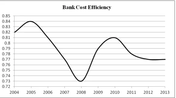
Concerning the evolution of bank efficiency over time, Figure 3 indicates an apparent reduction in cost efficiency during the years 2005 – 2008 with the lowest score in 2008 (0.73). The next two years are characterized by a positive trend (0.79 in 2009 to 0.81 in 2010). After the year 2010, bank cost efficiency decreases possibly because most of the European banks are exposed to the sovereign debt crisis.

[Insert Table 4 and Figure 3]

Regarding the accounting performance measures, we include ROE that is the return to shareholders on their equity. Our next measure of bank performance is the ROA that reflects the ability of managers to generate profits using banks assets indicating how efficient bank assets are managed. Finally, we employ NIM, which focuses on the profits earned from interest activities.

3.3. Measuring bank risk exposure

In this study, we employ various proxies of bank risk exposure. First, we employ the Altman’s Z-Score (Altman 1968) as a measure of bankruptcy risk. The Altman’s risk measure is derived from balance sheet values and is calculated as follows:

NO!PN+, = 1.2S_B+ 1.4S_C+ 3.3S_V+ 0.64S_Y+ 0.999S_Y (3) where SBis the ratio of working capital over total assets. Working capital is calculated

as the difference between current assets and current liabilities. Positive values of working capital indicated that the institution can cover its financial obligations. S_C is

14 the ratio of retained earnings over total assets and presents a measure of true profitability. SV is the ratio of earnings before interest and taxes over total assets. This measure

reflects the cash available for allocation to shareholders, creditors and government. S[

is the ratio of market value of equity to book value of liabilities while S_Y stands for the ratio of sales to total assets and presents the sales generating ability of the bank. Therefore, a greater value of Altman’s Z-Score indicate a lower probability of bankruptcy.5

As an additional measure of bank risk, we also consider an alternative of Altman’s Z-Score. We employ ZSCORE as proposed by Boyd and Graham (1986) according to the following formula: ZSCORE = (1 + ROE) / Standard Deviation of ROE. This measure has been used widely in banking literature (Barry et al. 2011; Bouvatier et al. 2014; Guo et al. 2015; Lepetit and Strobel 2015; Mamatzakis and Bermpei 2014; Mare et al. 2016; Radic et al. 2012; Soedarmono et al. 2013). The ZSCORE can be interpreted as an accounting based measure of the distance to default and implies that banks with a lower Z-Score have a higher risk of default.

Furthermore, we include the ratio of non-performing loans over total loans (NPL). We expect NPL to have a positive impact on bank capital buffer. Banks with increasing NPL will increase their capital buffer, as they are obligated to hold higher levels of loan loss provisions (Jokipii and Milne 2008). We also include the ratio of Off-Balance-Sheet items over total liabilities (OBS) as another measure for bank risk. OBS items are measured as the non-interest income and fee-generating from various contingent liabilities such as derivatives, letters of credit, insurance and other types of

15 traditional banking activities and securities underwriting. OBS items increase the risk exposure for a bank and therefore, we expect that banks with a greater amount of OBS items will hold higher a capital buffer. Finally, we include the ratio of risk-weighted assets over total assets (RWA), defined as the total amount of bank’s assets weighted for the credit risk according to Basel rules. We consider RWA as a proxy of bank risk as the allocation of bank assets among risk categories would define the quality of bank portfolio risk. (Berger 1995; Jacques and Nigro 1997; Jokipii and Milne 2011). Note that this measure of risk captures mainly bank’s exposure to the credit risk (Jokipii and Milne 2011).

3.4. Other control variables

As a measure of market discipline, we include a dummy variable DISCLSR that takes the value 1 for listed banks and 0 for unlisted. We expect that the observability of bank’s risk choices, as captured by this dummy variable, will increase the incentives for banks to hold regulatory capital above the minimum requirement. The main reasons are first, to reduce the risk of default and second to avoid being penalised by investors for choosing higher risk (Boot and Schmeits 2000; Nier and Baumann 2006).

We also include the explanatory variable SIZE, measured as the natural log of total assets, to detect differences in the level of the capital buffer because of the bank size. Size may have an impact on capital buffer due to the extent of bank diversification, cost of funding and investment opportunities. This relationship could be either positive or negative depending on how small and large banks adjust their capital buffer during the period under study. Size may have a negative impact on capital buffer, as large and well-diversified banks have a smaller probability of a sharp decline in their capital ratios.

16 Moreover, smaller banks may increase their capital buffer in order to accommodate difficulties to access capital markets in case of emergency (Ayuso et al. 2004; Francis and Osborne 2012; Jokipii and Milne 2008). A positive relationship might also exist, in particular, due to the financial crisis of 2008. This positive relationship between bank size and buffer is in line with the “franchise-value hypothesis” according to which bigger banks may reinforce their charter value during difficult times by enhancing their capital. Thus, it could be the case that during the period under study, larger banks, compared to small banks, will take advantage of economies of scale, diversification effects and easier access to capital markets to increase their capital and comply with the minimum requirements.

We also account for the concentration ratio (C5) in the banking industry by including the sum of the assets of the five largest banks as a share of all banks in each country and for each year. The impact of the concentration ratio on capital buffer could be either positive or negative. The sign depends on whether a low competition will increase or decrease the incentives for a higher capital (Nicoló et al. 2004).

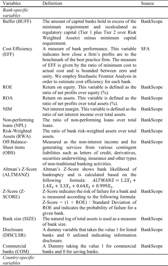
Furthermore, in order to eliminate the potential biases associated with having omitted variables, we employ a dummy variable that takes the value 1 for European Monetary Union countries and 0 otherwise (EMU). In addition, we include time dummies to capture any potential time effects and a dummy variable for commercial banks (COM) to account for any differences between commercial and saving banks (Casu and Girardone 2010). Table I in Appendix provides a brief description of the variables and the data sources, while Table 6 reports summary statistics for the key variables.

17 4. Methodology

4.1. Dynamic Panel Model

Following previous studies (Ayuso et al. 2004; Jokipii and Milne 2008), we employ partial adjustment process in order to account for costs of adjustments in the capital buffer. We consider bank-specific variables and country-specific variables as determinants of the capital buffer as analysed in the data section. We apply the two-step system generalized method of moments (GMM) estimator as developed by Arellano and Bover (1995) for a dynamic model of panel data.6 _{This methodology is preferred} for three main reasons. First, by taking the first differences for all variables, we eliminate the presence of any unobserved bank-specific effects. Second, we use the lagged dependent variable to capture the dynamic nature of capital buffer and third, by using GMM methodology, we account for the potential endogeneity of the explanatory variables. We consider as exogenous the country-specific variables and time dummies and as endogenous the bank-specific variables (Ayuso et al. 2004). The instruments chosen for the lagged endogenous variables are two-to-six period lags of the same variables. Furthermore, the results of the two-step system GMM estimator are tested by Hansen’s J diagnostic test for instrument validity and the test for the second-order autocorrelation of the error terms as suggested by Arellano and Bond (1991). Finally, we account for Windmeijer (2005) biased-corrected robust standard errors.

6 _{In this paper with use the xtbond2 stata command that implements the two-step system GMM estimator} with the Windmeijer (2005) correction to the reported standard errors. In the one-step system GMM robust standard errors are reported which are robust to heteroscedasticity. In two-step GMM error terms are already robust and Windmeijer (2005) correction is implemented to standard errors. Two-step uses the consistent variance co-variance matrix from first step GMM to reconstruct the weight matrix. Without this correction, the standard errors tend to be downward biased.

18 The model that we examine is the following:

\]44#,%= A?+ AB \]44#,%^B+ AC 344#,%+ AV NO!PN+,#,%+ A[ ,_"`a3#,% +

A_Y+)O_#,%+ A_b `\_<sub>#,%</sub>+ A<sub>c</sub>adN<sub>#,%</sub>+ A<sub>e</sub> fg_"`_]a3_#,% + A_h_g,3_#,%+

A_B?"`P_#,%+ A_BB"5_#,%+ A_BCjf)ja_#,% + klmn n''nokp + 2_#,% (4)

where the lagged value of the dependent variable (\]44#,%^B) captures the importance

of adjustment costs and we expect a positive and significant coefficient for this variable as stated in the hypothesis H1. 344#,% stands for bank efficiency, NO!PN+,#,% is

Altman’s Z-Score calculated according to Altman (1968) and measures the bank’s risk for bankruptcy, ,_"`a3#,% is an additional measure bank risk presenting the distance

from default. Other risk determinants that can affect bank capital buffer and we account for are +)O_#,%measured as the ratio of non-performing loans to total assets, `\__#,% which is the ratio of off-balance-sheet items to total liabilities and adN_#,%which stands for the ratio of risk-weighted assets to total assets.

We also consider the impact of market discipline employing the variable fg_"`_]a3#,% that takes the value one for listed banks and 0 for unlisted. _g,3#,%

stands for bank size measured as the natural log of total assets. "`P_#,% is an indicator variable that takes the value 1 for commercial banks and 0 otherwise, "5_#,% is the concentration ratio for the banking industry calculated as the sum of the assets of the five largest banks as a share of all banks in each country, jf)ja_#,%us the GDP growth in each country and 3P]#,% is an indicator variable that takes the value 1 for European

19 set of time dummies to capture the unobserved time effects. The error term 2_#,% consists of a bank-specific component I#, which is assumed to be constant over time and a white

noise s_#,%. Hence,2_#,% = I_# + s_#,% where I_# ~ iid (o,σµ2) ands_#,%~ iid (o,σε2). 4.2. Dynamic panel threshold model

Given the financial crisis of 2007 - 2008, we opt for a novel methodology that enables us to identify any potential regime changes in the relationship between capital buffer, bank performance and risk-taking. We employ the threshold methodology proposed by Hansen (1999) and developed by Kremer et al. (2013). This methodology uses the cross-sectional model employed by Caner and Hansen (2004), where the authors allow for endogeneity by using GMM estimators. Kremer et al. (2013) extended threshold analysis to a dynamic unbalanced methodology that identifies possible changes in the coefficient of the independent variables.

We employ the following threshold model:

\]44_#,%= I_#+ t_Bm_#,% g(S_#,%≤ v. + E_Bg(S_#,% ≤ v. + t_Cm_#,%g (S_#,% > v. + s_#,% (5) The subscript i refers to the individual banks and the subscript t indexes the time. \]44_#,% is the dependent variable, I_# is the bank-specific fixed effect and t_B and t_C the reverse regression slopes and based on these slopes we assume two regimes. S_#,% is the threshold variable and v is the threshold value, which distribute the observations above and below the threshold value composing the high and low regimes respectively. g is the indicator function that specifies the two regimes as defined by the threshold variable. Finally, s_#,% is the error term, which is assumed to be independent and identically distributed (iid) with mean zero and finite variance σ2_{. The model employed by Kremer}

20 et al. (2013) treats m_#,% as a vector of explanatory variables that includes a subset m1_#,% of exogenous variables uncorrelated with s#,% and a subset m2#,% of endogenous

variables correlated with s_#,%. Furthermore, Kremer et al. (2013) extend Hansen’s (1999) work by accounting for the regime dependent variable E_Bwhich represents the differences in the regime intercepts. According to Bick (2010), we include E_B as disregarding the regime intercepts would lead to biased estimates for both the regime coefficients and the threshold value.

In the first step, in order to estimate the predicted values, Kremer et al. (2013) following Caner and Hansen (2004) uses the reduced form of regressions for the endogenous variable as a function of instruments. In step two, the threshold value γ is estimated by using the predicted values of the endogenous variables in Eq. (5). In the third step, to obtain the slope parameters tB and tC, Eq. (5) is estimated via GMM for the threshold

value γ, where the threshold variable is replaced by its predicted values calculated in the second step. According to Caner and Hansen (2004), the optimal threshold is estimated via a minimizer of the sum of squared errors by using 2SLS estimator. Following Caner and Hansen (2004) and Hansen (1999), the 95% confidence interval of the threshold value is given by the Γ = [γ: LR(γ) ≤ C(α)]. Here, C(α) indicates the asymptotic distribution of the likelihood ratio (LR) statistic at 95% significance level.

5. Empirical Results

5.1.Panel regression results

We first propose to examine the association between capital buffer, performance and risk employing dynamic panel regressions for the model specified in equation (4). We start our analysis with this methodology to capture the dynamic nature of capital buffer

21 and to account for the potential endogeneity of the explanatory variables. Besides the dynamic panel analysis, we propose a threshold methodology that identifies potential regime switches in the underlying relationships, while at the same time it maintains all the advantages of the dynamic panel analysis as discussed previously. Therefore, our main motivation for the use of the threshold analysis is to identify any changes in the relationships between the variables because of the financial crisis of 2008.

Dynamic panel results are presented in Table 6 and 7. In Table 6, we use the cost efficiency as a performance measure. We add the control variables gradually to see the individual impact of the main variables. Model (3) includes ALTMANZ as the main measure of bank risk, while in Model (4) we use ZSCORE as part of sensitivity analysis of an alternative bank risk measure. Next, in Models (5) - (7) we employ NPL, OBS and RWA variables respectively. Finally, Model (8) accounts for all bank and country-specific variables simultaneously. The cost of adjustment as captured by the coefficient of the lagged dependent variable \]44#,%^Bis positive and highly significant in all

specifications. These results confirm hypothesis H1 suggesting that banks need time to adjust their current capital buffer. The coefficient of \]44_#,%^Bchanges across different models when we include other control variables. Adding all bank and country-specific variables in Model (8), the speed of adjustment increases from 0.188 in Model (1) to 0.572 in Model (8). The speed of adjustment of 0.572 in Model (8) indicates that when we account for other determinants of bank capital buffer, banks converge to the target buffer with a rate of 57.2% per annum.

In terms of regression estimates, the coefficient of cost efficiency (EFF) is positive and significant at 1% level (see Models (2) and (7)). In Model (8) which includes all control

22 variables, EFF exerts a positive impact on bank capital buffer at 5% level. These results are in line with our second hypothesis H2 indicating that higher efficiency leads to a greater capital accumulation (Fiordelisi et al. 2011). This finding is in agreement with the pecking order theory which argues that institutions prefer to use internal sources of funding rather than external sources (Myers and Majluf 1984). Furthermore, this positive relationship between bank efficiency and capital buffer could be explained by the “franchise-value hypothesis” according to which due to the income effect of high cost efficiency, banks will choose to hold a higher capital to protect their reputation and charter value (Berger and Bonaccorsi di Patti 2006). 7

As regards the impact of bank risk measures on capital buffer, ALTMANZ carries a positive and highly significant coefficient in Model (3) and Model (8). This positive relation between ALTMANZ and BUFF suggests that banks that are less likely to default (lower risk) hold a greater capital buffer. Note that this relationship is significant at 1% in Model (8). These findings reinforce the “franchise-value hypothesis”. Stable banks with a lower risk of default have higher charter value (Jokipii and Milne 2011) and therefore, banks with high Z-Score will sustain their value by maintaining a higher capital buffer.

The OBS variable exerts a positive impact on bank capital buffer at 10% level in Models (6) and (8) providing evidence for hypothesis H3 and supports the “regulatory hypothesis” according to which banks with greater off-balance sheet activities prefer to hold higher capital buffer as a cushion against unexpected losses. We also report a

7 _{Franchise or charter value of a bank is defined as the value that would be foregone due to a bankruptcy. According} to this theory there is ambiguous relationship between bank capital and risk taking. The higher risk can increase the probability of default and therefore encourage banks to raise their capital. This has been broadly discussed by Boot and Schmeits (2000).

23 positive and at 1% level significant coefficient for the bank size. Existing literature (Ayso et al. 2004; Guidara et al. 2013; Jokipii and Milne 2008; Stolz and Wedow 2011) provide evidence for the too-big-to-fail phenomenon according to which larger banks expect government support in an event of distress and thereby might keep lower capital buffer. Furthermore, according to this strand of literature, larger banks benefit from economies of scale and diversification effects. Therefore, larger banks have easier access to capital markets and a lower probability of a sharp drop in their capital ratios. In contrast, small banks might need to maintain a greater capital buffer to deal with difficulties to draw on capital markets. In this study, which covers the years of the financial meltdown of 2007 – 2008, we report results that are in line with the “franchise-value hypothesis”. Thus, larger institutions would protect their sustainability during difficult periods by ensuring their capital adequacy.8

All models pass the Hansen standard validity tests of the instruments used in the regressions. Moreover, AR(2) p-values reject the presence of second-order correlation in the error terms, as should be if the residuals in levels are white noise.

[Insert Table 6]

In a further analysis, we use dynamic panel regressions to examine the relationship between capital buffer and performance. Model (1) in Table 7 employs bank efficiency, Model (2) uses the ROE as an indicator of bank profitability, Model (3) examines the relationship between the capital buffer and ROA while Model (4) includes NIM.

8 _{Banks that violate the minimum capital requirements lose part of their charter value (Flannery and} Rangan 2004; Stolz and Wedow 2011). Thus, larger banks will take advantage of the economies of scale, diversification effects and the easier access to capital markets to maintain a higher capital buffer.

24 Models (5) - (7) report the simultaneous impact of the efficiency and one of the other performance measures on buffer.

Model (2) documents a positive relationship between ROE and capital buffer at 1% level. Consistent with the impact of EFF on buffer in Table (6), this result provides further evidence for both the “franchise-value hypothesis” and the pecking order theory. Therefore, more profitable banks that accumulate equity through retained earnings, may hold greater capital buffer, especially when raising capital is difficult. Arguably, less profitable banks suffering from a greater cost of issuing equity might maintain a lower capital buffer. These results could be compared with those obtained from Nier and Baumann (2006) who suggest that ROE can enhance capital buffer. Similar results documenting a positive relationship between profitability and capital have been found in Berger (1995) and Flannery and Rangan (2008) for the 1980s and 1090s respectively.9

As regards the impact of the other control variables on buffer, after employing ROE as a performance measure, ALTMANZ and SIZE maintain their positive and highly significant impact on buffer. The significant coefficient of ALTMANZ indicates that even when we account for bank performance with ROE, lower likelihood of bankruptcy leads to higher capital buffer. The positive coefficients of NPL and OBS in Models (4) – (7) provide evidence in favour our hypothesis H3 for a positive relationship between risk and capital buffer supporting the “regulatory hypothesis”.

9 _{Alfon et al. (2004), Ayuso et al. (2004) and Jokipii and Milne (2008) document a negative association} between capital and past values of the return on equity. In this strand of literature the return on equity is used as an indicator of bank’s cost of raising equity capital. However, in this study and consistent with Berger (1995), Nier and Baumann (2006) and Flannery and Rangan (2008) the return on equity is used as an indicator of firm profitability.

25 Next, Models (5) – (6) report the impact of bank efficiency on buffer when we include additional measures of performance. Models (5) – (7) employ both EFF and one of the other accounting performance measures (ROE, ROA and NIM) in the regressions. Estimated results suggest that even when we account for other accounting performance measures, bank efficiency exerts a positive and at least at 5% level significant impact on the capital buffer. These findings imply that the inclusion of other performance measure does not affect our regression results.

[Insert Table 7]

5.2.Threshold estimations

5.2.1. The capital buffer and efficiency nexus

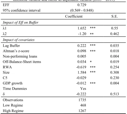
Our sample for threshold estimation consists of 1,735 observations for 314 banks over the period 2005-2013. The results for the empirical relationship between buffer and efficiency are presented in Table 8. We find a threshold variable of 0.729 for bank efficiency. This threshold value splits our sample into two regimes. The low regime includes 468 banks with efficiency scores less than 0.729. The estimated coefficient t_B indicates that for banks that fall in the low efficiency regime, efficiency exerts a positive impact on buffer at 1% level. This result suggests that for the relatively less efficient banks, an increase in efficiency enhances bank capital buffer. The high regime consists from 1267 banks with efficiency scores greater than the threshold value. The negative sign of the estimated coefficient tC implies that for banks in the high regime, efficiency

has a negative impact on buffer at 5% level.

A striking result of this analysis is that the relationship between buffer and efficiency is characterized by a structural breakpoint, indicating that the impact of efficiency on

26 capital buffer depends on the level of bank’s efficiency. The positive coefficient for banks falling in the low regime suggests that the relatively less efficient banks use their increased efficiency to accumulate higher capital buffer. This finding confirms hypothesis H2 and is in line with the “franchise-value hypothesis”. According to this theory, banks that are more efficient tend to hold a higher capital to protect their future income derived from high efficiency (Berger and Bonaccorsi di Patti 2006). Conversely, the negative coefficient for the relatively more efficient banks provides evidence in favour of the “efficiency-risk hypothesis” suggesting that a higher level of efficiency might substitute to capital against unexpected losses (Berger and Bonaccorsi di Patti 2006). These findings are in agreement with Altunbas et al. (2007), Berger and Bonaccorsi di Patti (2006) and Kwan and Eisenbeis (1997) who document a negative relationship between capital and efficiency. Furthermore, our results are similar to Ayuso et al. (2004) and Jokipii and Milne (2008) who find an inverse relationship between bank performance and capital buffer.

Overall, this study complements prior literature on the association between bank capital buffer and efficiency documenting a breakpoint in the underlying relationship. We show that for the relatively less efficient banks (low regime) the capital buffer choice dominates over the substitution effect, suggesting that relatively less efficient banks choose to maintain more capital buffer to protect their franchise value. In contrast, for the relatively more efficient banks (high regime), the substitution effect dominates over the capital buffer choice as an increasing efficiency may substitute for capital in protecting the firm from financial distress.

27 In line with the results obtained from the dynamic panel regressions in Table 7, the coefficient of the lagged value of capital buffer (Lag Buffer) is positive at 1% level, confirming hypothesis H1. Furthermore, Altman’s Z-Score carries a positive and at 1% significant level coefficient suggesting that banks with a lower risk of default accumulate greater capital buffer. RWA exerts a negative impact on buffer at 1% level indicating that banks with a greater portfolio of risk-weighted assets face difficulty in increasing their capital above the minimum requirements. The negative relationship between buffer and RWA also suggests that banks are forced to increase their capital buffer by reducing their risk-weighted assets (Shim 2013). Finally, the positive impact of bank size on capital buffer suggests that larger banks might hold higher buffer as a sign of solvency due to their easier access to capital markets.

[Insert Table 8]

Table 9 presents the evolution of banks in low and high regimes for the period 2005 – 2013. One can notice a negative trend in the percentage of banks with relatively higher efficiency scores for the years 2006 - 2008 (90% in 2005 decreases to 88% in 2006 to 82% in 2007 and 65% in 2008). Although, for the years 2009 – 2010 there is a significant recovery in the number of banks that fall in the high efficiency regime (from 65% in 2008 to 75% in 2009 and 80% in 2010), the trend in the following years is negative. These results are supported by the impact of the financial crisis of 2007 – 2008 on the banking sector. The reduction in the number of banks with efficiency above the threshold value mirrors the deteriorating performance of banks during the crisis.

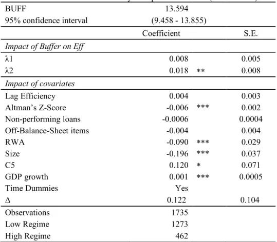
28 In a further analysis, we account for the impact of the capital buffer on bank efficiency. Therefore, we employ the threshold methodology using the buffer as a threshold variable and the efficiency as a dependent variable. The impact of the buffer on efficiency is presented in Table 10. The estimated buffer threshold is 13.594. The low regime consists of 1,273 banks with relatively low capital buffer while the high regime consists of 462 banks. The coefficient t_C for banks in the high regime is significant at 5% level. Our findings could be compared with those of Fiordelisi et al. (2011) who find that an increase in bank capital leads to an efficiency improvement and with and Kwan and Eisenbeis (1997) who show that better capitalized banks exhibit higher level of efficiency than less-capitalized banks.

Furthermore, the negative and significant at 1% level coefficient of Altman’s Z-Score may suggest that banks with a lower risk of default do not consider that much cost efficiency leading to lower efficiency scores. RWA exerts a negative impact on efficiency at 1% level. The impact of bank size on efficiency is negative implying that bank efficiency decreases as bank size increases.10

[Insert Table 10]

The evolution of banks in the low and high regimes over the sample period is presented in Table 11. It is obvious that the percentage of banks classified in low regime is consistently above the percentage of banks in the high regime. Table 11 shows a negative trend in the percentage of banks with high capital buffer for the years between 2006 and 2008 (27% in 2006 to 21% in 2007 and 23% in 2008). These results could be

10 _{This finding is supported by Stiroh and Rumble (2006) who show that size is negatively correlated with} efficiency for both domestic and foreign banks. The authors explain this relation through the agency costs, bureaucratic processes and other costs of managing extremely large institutions.

29 explained by the high cost of raising capital during distress (Campbell 1979). Our findings suggest that the ability of banks to accumulate regulatory capital over the minimum requirement has deteriorated due to the financial crisis of 2007 – 2008.

[Insert Table 11]

5.2.2. The capital buffer and Altman’s Z-Score nexus

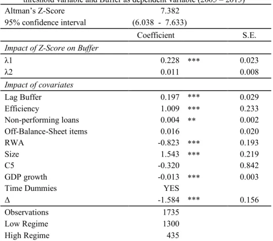
We further examine the relationship between bank capital buffer and risk of default as measured by the Altman’s Z-Score. High values of Altman’s Z-Score indicate more stable banks and thus, lower risk of default. Table 12 presents threshold estimation results using the buffer as the dependent variable and Altman’s Z-Score as the threshold regime variable. The threshold value for the Altman’s Z-Score is 7.382. This value splits our sample into the low regime, which consists of banks with relatively greater risk of default, and the high regime consisting of more stable banks. The coefficient tB is

positive and significant at 1% level while the impact of Altman’s Z-Score on capital buffer is insignificant for banks in the high regime. These results are in line with those obtained by the dynamic panel regressions in Table 7, indicating that banks with relatively lower Altman’s Z-Score and therefore, a higher risk of default, will choose to hold a higher capital buffer. Our findings provide evidence for the “regulatory hypothesis” according to which regulators encourage banks with a higher risk exposure to hold a higher capital buffer.

Concerning the impact of the other bank-specific variables on buffer, the estimated results in Table 12 are in line with those of Table 8 where the threshold variable was the efficiency. The lagged value of buffer, efficiency, non-performing loans and bank size exert a positive impact on capital buffer. Finally, RWA carries a negative and 1%

30 significant sign, suggesting that a greater portfolio of risky assets curbs bank’s ability to accumulate capital above the minimum requirements.

[Insert Table 12]

The evolution of banks in low and high regimes over time is presented in Table 13. The percentage of banks in the low regime is above the percentage of banks in the high regime. These results could mirror the negative impact of the financial crisis of 2007 – 2008 showing that over this period at least the 70% of the banks in our sample are characterized with relatively greater likelihood of default.

[Insert Table 13]

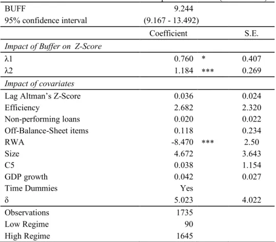
To examine the impact of capital buffer on bank default risk, we employ the threshold methodology using Altman’s Z-Score as the dependent variable and buffer as the threshold regime variable. Table 14 presents the estimated results. The threshold value of capital buffer is 9.244 and splits our sample in the low regime that consists of banks with relatively low buffer and the high regime with the relatively well-capitalised banks. Both regime-dependent coefficients ( t_B and t_C) of buffer are positive and significant at 10% and 1% level respectively.

These findings show that an increase in buffer increases Altman’s Z-Score and therefore, decreases the risk of default. Our results are in line with Kwan and Eisenbeis (1997) and Guidara et al. (2013) who find that better-capitalized banks tend to have lower risk exposure. More importantly, these results suggest that the greater the minimum capital requirement, the weaker the incentives for banks to engage in risky activities leading to a lower risk of default. Therefore, these results support that the implementation of

31 minimum capital requirements by Basel Committee, has succeeded in its main aim of enhancing bank stability.

[Insert Table 14]

Finally, Table 15 shows that the percentage of the relatively well-capitalised banks is above that of the relatively low capitalized. After the year 2007, there is a negative trend (90% in 2005 to 85% in 2007). This might be due to the costly capital during the crisis of 2007 – 2008 that renders difficult for banks to increase their regulatory capital.

[Insert Table 15] 6. Sensitivity analysis: A panel-VAR model

As part of sensitivity analysis that takes into account possible endogeneity among the main variables of our modelling, we employ a panel-VAR model where all main variables (i.e. except control variables) enter a system of equations as endogenous. Such model would facilitate the identification of causality directions between the main variables in a dynamic way. As a first step, we need to decide the optimal lag order j of the variables. We seek for the optimal lag order following Lutkepohl (2006). We also apply the Akaike Information Criterion (AIC) and the Arellano-Bond AR tests. The optimal lag identified is equal to one. Sargan test reports for lag equals to one the null hypothesis is not rejected.11 _{Therefore, we employ a panel-data autoregression} methodology by using a first order 3x3 panel-VAR model following Love and Zicchino (2006) 12_:

11 _{Results are available upon request. Note that the ordering of variables could also be of importance. We} test for the reverse ordering and results remain similar. Results are available under request.

32 , i =1,…, N, t=1,…,T. (8) Where Xit is a vector of three main variables of this analysis that is the bank capital buffer, bank efficiency and Altman’s Z-Score. Thus, Φ indicates a matrix of coefficients (3x3), whilst µi a vector of bank-specific effects and ei,tiid residuals. For estimation

purposes, to account for endogeneity we follow Love and Zicchino (2006) employing the Arellano-Bond system-based GMM estimator. Essentially, the panel-VAR is a system of the following equations:

\]44_#%= A_B?+ ∑{_D|BA_BB\]44_#%^D+ ∑{_D|BA_BC344_#%^D+ ∑{_D|BA_BVNO!PN+,_#%^D+ n_B#,%

344_#%= A_C?+ ∑{_D|BA_CB\]44_#%^D+ ∑{_D|BA_CC344_#%^D+ ∑{_D|BA_CVNO!PN+,_#%^D+ n_C#,%

NO!PN+,_#%= A_V?+ ∑_D|B{ A_VB\]44_#%^D+ ∑{_D|BA_VC344_#%^D+ ∑{_D|BA_VVNO!PN+,_#%^D+ n_V#,%

(9)

The above system of equations has a moving average (MA) representation as a function of a set of present and past residuals e1, e2, and e3. Given possible endogeneity, these

equations could be correlated and thereby the coefficients of the MA representation are not meaningful. A way to have meaningful estimations is to orthogonalise the residuals opting for the Cholesky decomposition of the covariance matrix. In addition, we introduce fixed effects to ensure heterogeneity in the levels.13

6.1.1. Panel Impulse response functions (IRFs)

13_{Following Love and Zicchino (2006) we apply the Helmert procedure in the data set. That is the data} we are forward mean differenced.

t i it i it

=

+

F

X

+

e

X

µ

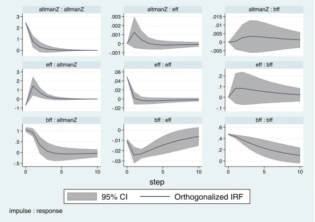
33 Figure 4 presents impulse-response functions (IRFs) and the 5% error banks generated by Monte Carlo simulation for a panel VAR of the following ordering of variables Altman’s Z-Score (ALTMANZ), bank efficiency (EFF) and capital buffer (BFF).14

[Insert Figure 4]

From the first row of Figure 4, the last plot shows that the effect of one standard deviation shock of Altman’s Z-Score on the buffer is positive, while this effect becomes less pronounced after the fourth year. This result is in line with the main results in Tables 6 and 7 providing further support for the “franchise-value hypothesis”. According to this hypothesis, banks with a lower risk of default have higher charter value (Jokipii and Milne 2011) and will sustain their value by holding a higher capital buffer.

Next, one can notice from the second row, last plot that the response of the capital buffer to one standard deviation shock of efficiency is positive as well. It picks after the first two periods and converges to the equilibrium thereafter. These results are in line with our main results obtained in Tables 6 and 7. Thus, the “franchise-value hypothesis”

dominates over the “efficiency-risk hypothesis” indicating that banks with higher efficiency choose to hold a higher buffer to protect their charter value and future earnings.

In the case of Altman’s Z-score, the panel-VAR methodology appears to confirm the findings of Table 14 (see Figure 4, the first plot in the last row that reports the response of Altman’s Z-Score to one standard deviation shock of buffer). The response is positive

14 _{As the ordering of variables in the panel VAR is not without significance we also estimate the system} of equations, opting for the reverse ordering of variables. Results remain are available under request and confirm the present findings.

34 across the whole period and in agreement with the positive coefficients λ1 and λ2 of both regimes in Table 14. Thus, the panel-VAR results show that a higher capital buffer enhances bank stability by reducing the risk of default (increasing Altman’s Z-Score). Finally, the second plot in the third row of Figure 4 shows that the effect of one standard deviation shock of buffer on efficiency is negative and it converges towards the equilibrium after the first period. This finding comes in contrast with our previous results in Table 10. However, this result needs to be interpreted with some caution as the response crosses the zero line and might imply a loss of significance.

Next, we present VDCs, which show the percent of the variation in one variable that is explained by the shock to another variable, accumulated over time. The variance decompositions show the magnitude of the total effect. We report the total effect accumulated over 10 years. Longer time horizons produced equivalent results. Table 16 presents the VDCs estimations. These results come in agreement with those reported by the IRFs, and provide further evidence that the level of efficiency explains the variation of buffer, though mostly it is buffer itself that explains its variation. Particularly, 3.43% of the forecast error of capital buffer after ten years is explained by shocks in the EFF variable. Furthermore, the VDCs results show that the level of buffer explains almost the half (50.8%) of the variation of efficiency. Finally, both capital buffer and efficiency are significant determinants of bank’s risk of default. Around 17.75% of the forecast error variance of ALTMANZ after 10 years is captured by BFF disturbances and about 26.33% by EFF disturbances.

35 7. Conclusion

This study empirically addresses the association between bank capital buffer, performance and risk. Using a sample of EU-27 banks over the period between 2004 and 2013, the findings of this study could be of interest to both supervisory authorities and bank managers. Given that our sample covers the financial crisis of 2007 – 2008, we employ the dynamic panel threshold methodology as developed by Kremer et al. (2013). Results show different regimes over the sample period. A strong positive impact of bank performance on the capital buffer is reported for banks in the low performance regime, while for the relatively better performing banks an improvement in the performance decreases the capital buffer. Moreover, threshold results indicate a positive impact of buffer on bank performance. These findings provide evidence that the regulatory framework as regards the capital adequacy requirements can enhance bank performance. Furthermore, threshold analysis shows that capital buffer exerts a strong positive impact on bank stability. The positive relationship between buffer and Altman’s Z-Score suggests that the implementation of minimum capital requirements might have succeeded in its main aim of creating a more stable banking system and reducing banks’ default risk.

Notably, we find changes in the percentage of banks in each threshold regime during and after the financial crisis of 2007 – 2008. There is an increasing trend in the percentage of banks in the low performance regime over time, especially after the years 2007 – 2008. This finding indicates that banks in the EU-27 region experienced a period of substantial performance deterioration. Moreover, the number of banks in the low capital buffer regime is consistently above the number of banks in the high regime during the financial crisis. Given the high cost of raising capital during the economic

36 downturn, EU-27 banks accumulate lower capital during the recession period. These results are of some value for managers and policy makers in particular. Our findings clearly indicate that the impact of capital requirements is different for banks with different performance and risk characteristics.

37 References

Alali F, Jaggi B (2011) Earnings versus capital ratios management: Role of bank types and SFAS 114. Rev Quant Financ Acc 36:105-132

Albertazzi U, Gambacorta L (2009) Bank profitability and the business cycle. J Financ Stab 5:393-409

Alfon I, Argimon I, Bascuñana-Ambrós P (2004) What determines how much capital is held by UK banks and building societies?. London: Financial Services Authority.

Altman EI (1968) Financial ratios, discriminant analysis and the prediction of corporate bankruptcy. J Financ 23:589–609

Altunbas Y, Carbo S, Gardener EPM, Molyneux P (2007) Examining the Relationships between Capital, Risk and Efficiency in European Banking. Eur Financ Manag 13:49-70 Arellano M, Bover O (1995) Another look at the instrumental variable estimation of

error-components models. J Econometrics 68:29-51

Athanasoglou PP, Brissimis SN, Delis MD (2008) Bank-specific, industry-specific and macroeconomic determinants of bank profitability. J Int Financ Market Instut Money 18:121-136

Avramidis P, Pasiouras F (2015) Calculating systemic risk capital: A factor model approach. J Financ Stab 16:138-150

Ayuso J, Pérez D, Saurina J (2004) Are capital buffers pro-cyclical?: Evidence from Spanish panel data. J Financ Intermed, 13:249-264

Barry TA, Lepetit L, Tarazi A (2011) Ownership structure and risk in publicly held and privately owned banks. J Bank Financ 35:1327-1340

Baule R (2014) Allocation of risk capital on an internal market, Eur J Oper Res 234:186-196 Baumann U, Nier E (2003) Market discipline and financial stability: some empirical evidence.

Financ Stab Rev 14:134-141

Beccalli E, Casu B, Girardone C (2006) Efficiency and stock performance in European banking. J Bus Finance Account 33:245-262

Berger AN, (1995) The relationship between capital and earnings in banking. J Money Credit Bank 27:432–456

Berger AN, Bonaccorsi di Patti E (2006) Capital structure and firm performance: A new approach to testing agency theory and an application to the banking industry. J Bank Financ 30:1065-1102

Berger AN, Humphrey DB (1997) Efficiency of financial institutions: International survey and directions for future research. Eur J Oper Res 98:175-212

Berger AN, Leusner JH, Mingo JJ (1997) The efficiency of bank branches. J Monet Econ 40:141-162

Bick A (2010) Threshold effects of inflation on economic growth in developing countries. Econ Lett 108:126-129

Boot AWA, Schmeits A (2000). Market Discipline and Incentive Problems in Conglomerate Firms with Applications to Banking. J Financ Intermed 9:240-273

Bouvatier V, Lepetit L, Strobel F (2014) Bank income smoothing, ownership concentration and the regulatory environment. J Bank Financ 41:253-270

Buser SA, Chen AH, Kane EJ (1981) Federal Deposit Insurance, Regulatory Policy, and Optimal Bank Capital. J Financ 36:51-60

Calormiris CW, Wilson B (1998) Bank Capital and portfolio management: The 1930's capital crunch and scramble to shed risk (No. w6649). National Bureau of Economic Research. Campbell TS (1979) Optimal Investment Financing Decisions and the Value of Confidentiality.

J Financ Quant Anal 14:913-924

Caner M, Hansen BE (2004) Instrumental Variable Estimation of a Threshold Model. Econometric Theory 20:813-843

Casu B, Girardone C (2010) Integration and efficiency convergence in EU banking markets. Omega 38:260-267