An Option Pricing Formula for the GARCH. Diffusion Model

(1)

An Option Pricing Formula for the GARCH

Diffusion Model

Claudia Ravanelli

Submitted for the degree of Ph.D. in Economics

University of Lugano, Switzerland

Prof. G. Barone-Adesi, University of Lugano, advisor

Prof. M. Chesney , University of Zurich

Prof. P. Vanini, University of Lugano

(2)

(3)

Acknowledgments

It is a great pleasure to thank Professor Giovanni Barone-Adesi, my thesis advisor, for invaluable suggestions and discussions and for his support during the last three years.

I am grateful to Professor Paolo Vanini for his useful comments and suggestions and for accepting to be a member of the thesis committee.

I really wish to thank Professor Marc Chesney for accepting to be co-examiner of this work. Thanks go to my friends Francesca Bellini, Ettore Croci, Silvia Cappa, Talia Cicognani, Clizia Lonati and Silvia Zerbeloni for making everyday life enjoyable.

My gratitude to my mom Silvana and to my brother Renato for their continuous support during these years.

(4)

List of Figures

2.1 c3effect. Percent Bias = 100 (Cegd−Cbs) for different maturities and parameter values ofc3,

whenS0= 100,r=d= 0;dV = (0.09−4V)dt+c3V dW,V0= 0.0225. . . 33 2.2 c∗

2effect. Percent Bias = 100 (Cegd−Cbs) for different maturities and parameter values ofc∗2,

whenS0= 100,r=d= 0;dV = (0.9−c2∗V)dt+ 1.2V dW,V0= 0.0225. . . 34 2.3 c1effect. Percent Bias = 100 (Cegd−Cbs) for different maturities and parameter values ofc1,

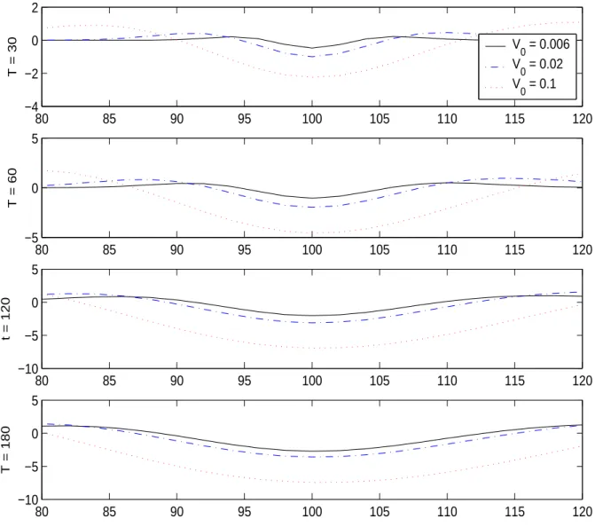
whenS0= 100,r=d= 0;dV = (c1−4V)dt+ 1.2V dW,V0= 0.0225. . . 35 2.4 V0effect. Percent Bias = 100 (Cegd−Cbs) for different maturities and initial varianceV0, when

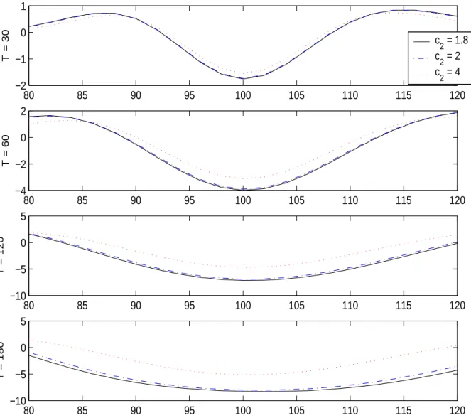
S0= 100,r=d= 0;dV = (0.09−4V)dt+ 1.2V dW.. . . 36 2.5 Volatility smiles for maturities of 30, 60, 90 and 120 days and the parameter choiceS0= 100,

r=d= 0;dV = (0.09−4V)dt+ 1.2V dW,V0= 0.0225, as in Table 2.5. . . 37 2.6 Volatility Surface for maturitiesT ∈[30,120] days, strikes K ∈ [90,110] and the parameter

choiceS0= 100,r=d= 0;dV = (0.09−4V)dt+ 1.2V dW,V0= 0.0225, as in Table 2.5. . 38 2.7 Relative height of volatility smiles of Mark-Dollar call options (1985-1992) . . . 39

(7)

3.1 Density estimates of the continuous time parametersc1 = 0.18,c2 = 2 and c3 = 1.2 of the

GARCH diffusion model (1.7)–(1.8) inferred by the parameter estimates of the discrete time GARCH-M model (3.1) at two-daily, daily and two-hourly sampling frequencies. Sample size 10 years. . . 46 3.2 Density estimates of the continuous time parametersc1 = 0.18,c2 = 2 and c3 = 1.2 of the

GARCH diffusion model (1.7)–(1.8) inferred by the parameter estimates of the discrete time GARCH-M model (3.1) at two-daily, daily and two-hourly sampling frequencies. Sample size 20 years. . . 47 3.3 Density estimates of the continuous time parametersc1 = 0.18,c2 = 2 and c3 = 1.2 of the

GARCH diffusion model (1.7)–(1.8) inferred by the parameter estimates of the discrete time GARCH-M model (3.1) at two-daily, daily and two-hourly sampling frequencies. Sample size 40 years. . . 48 3.4 DM/US daily exchange rates from December 1988 to December 2003.σ2

t is defined in equations

(3.1). . . 49 3.5 DM/US daily exchange rates from January 1985 to October 1988. σ2

t is defined in equations

(8)

List of Tables

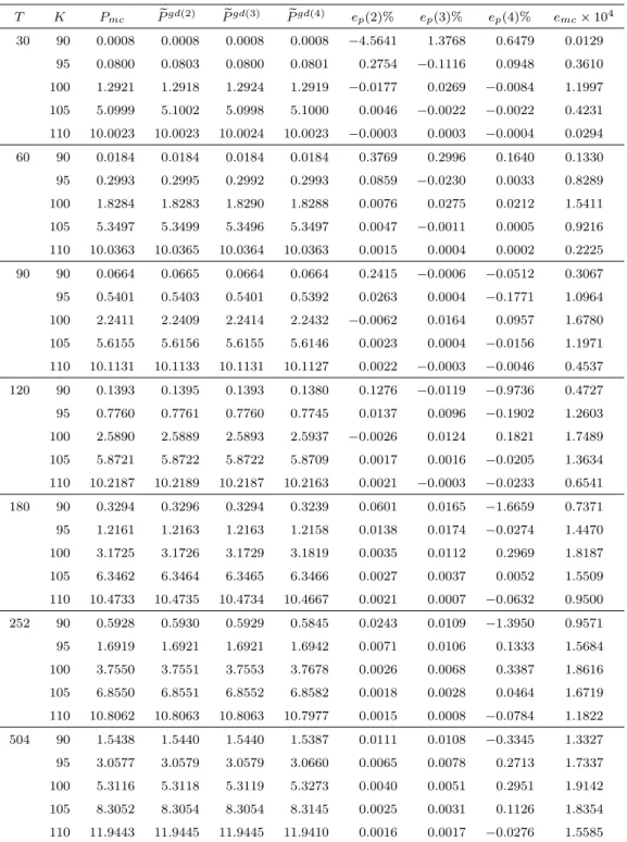
2.1 PmcMonte Carlo put prices computed byN = 106simulations;Pegd(i)GARCH diffusion put prices approximated by (2.10) truncated up to orderi-th, fori= 2, 3, 4;ep(i)% = 100(Pegd(i)₋_P_mc)_/P_mc;_e

mcMonte Carlo standard error. Model parameters: S0= 100, r=d= 0;dV = (0.16−18V)dt+ 1.8V dW,V0= 0.16/18. . . 28

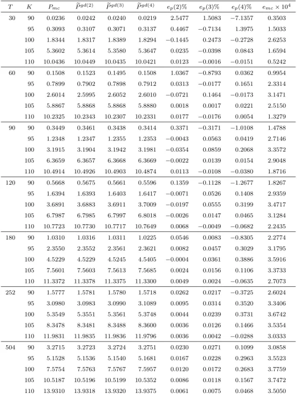
2.2 PmcMonte Carlo put prices computed byN = 106simulations;Pegd(i)GARCH diffusion put prices approximated by (14) truncated up to orderi-th, for i= 2, 3, 4; ep(i)% = 100(Pegd(i)₋_P_mc)_/P_mc;_e

mcMonte Carlo standard error. Model parameters: S0= 100, r=d= 0;dV = (0.53−29.23V)dt+ 3.65V dW,V0= 0.53/29.23. . . 29

2.3 PmcMonte Carlo put prices computed byN = 106simulations;Pegd(i)GARCH diffusion put prices approximated by (14) truncated up to orderi-th, for i= 2, 3, 4; ep(i)% = 100(Pegd(i)₋_P

mc)/Pmc;emcMonte Carlo standard error. Model parameters: S0= 100, r=d= 0;dV = (0.18−2V)dt+ 0.8V dW,V0= 0.18/2. . . 30

2.4 PmcMonte Carlo put prices computed byN = 106simulations;Pegd(i)GARCH diffusion put prices approximated by (14) truncated up to orderi-th, for i= 2, 3, 4; ep(i)% = 100(Pegd(i)₋_P_mc)_/P_mc;_e

mcMonte Carlo standard error. Model parameters: S0= 100, r=d= 0;dV = (0.18−2V)dt+ 1.2V dW,V0= 0.18/2. . . 31

(9)

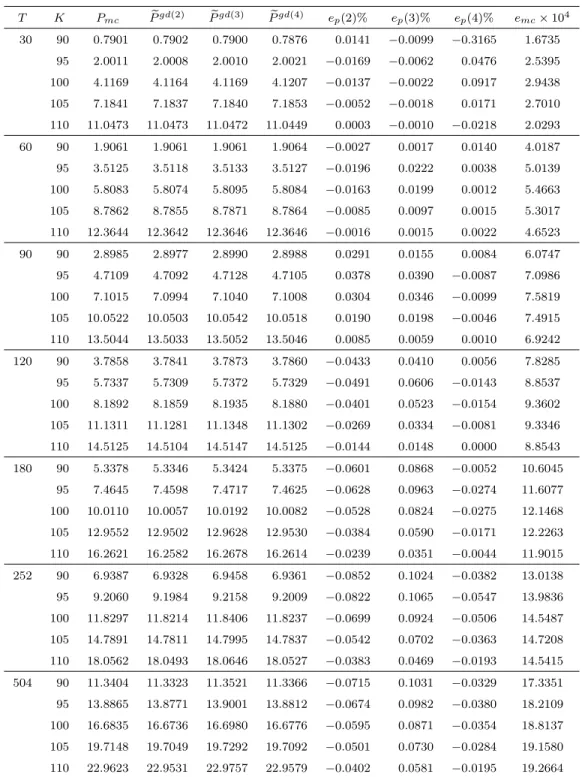
2.5 PmcMonte Carlo put prices computed byN = 106simulations;Pegd(i)GARCH diffusion put prices approximated by (14) truncated up to orderi-th, for i= 2, 3, 4; ep(i)% = 100(Pegd(i)₋_P

mc)/Pmc;emcMonte Carlo standard error. Model parameters: S0= 100, r=d= 0;dV = (0.09−4V)dt+ 1.2V dW,V0= 0.09/4. . . 32

3.1 Bias RMSE First panel: sample size 10 years; second panel: sample size 20 years; third panel: sample size 40 years . . . 44 3.2 Summary statistics (mean, variance, kurtosis and inter quartile range) of DM/US

ex-change rates daily log-returns. . . 44 3.3 GARCH(1,1)-M estimates for DM/US daily exchange rate from December 1988 to

De-cember 2003. Zt,µ,ω,αandβ are defined in equations (3.1). a_{Ljung-Box test follows} χ2_{(15) with the 0}_._{05 critical value being 25. . . .} ₄₄

3.4 GARCH(1,1)-M estimates for DM/US daily exchange rates from January 1985 to Oc-tober 1988. Zt, µ,ω,αand β are defined in equations (3.1). a _{Ljung-Box test follows} χ2_{(15) with the 0}_._{05 critical value being 25. . . .} ₄₅

(10)

Introduction

In this thesis, we study European option prices under a stochastic volatility model, where the asset price follows a geometric Brownian motion with instantaneous variance driven by a GARCH diffusion process.

Stochastic volatility models were introduced by Hull and White (1987), Scott (1987) and Wig-gins (1987) to overcome some drawbacks of the Black and Scholes (1973) and Merton (1973) model. Since Mandelbrot (1963) and Fama (1965) it was kwon that speculative log-returns are uncorrelated, not independent with a leptokurtic distribution and conditional variance changing randomly over time. Moreover, empirical studies on implied volatility (cf., for instance, Lantane and Rendleman, 1976, Beckers, 1981, and Canina and Figlewski, 1993) show a significant discrepancy between market and Black and Scholes prices. Implied volatilities vary with strike price and time to maturity of the options contract whereas in the Black and Scholes model the volatility is assumed to be constant.

Stochastic volatility models allow to account for random behaviors of implied and historical vari-ances and generate some log-returns features observed in empirical studies. Unfortunately, under stochastic volatilities closed or analytically tractable option pricing formulae are difficult to derive even for European options. The Hull and White (1987) and Heston (1993) models have an analyti-cal approximation and a quasi analytianalyti-cal formula to price European options, respectively. For other stochastic volatility models numerical methods are used.

(11)

In this thesis, we derive an analytical closed-form approximation for European option prices under the GARCH diffusion model, where the price is driven by a geometric process and the variance by an uncorrelated mean reverting geometric process. Our formula is related to the Hull and White (1987) option pricing series and involves the conditional moments of the integrated variance over the time to maturity. We show, using Monte Carlo simulations, that our approximation formula is accurate across several strike prices and times to maturity, it is easy to implement and allows to study the implied volatility and the volatility risk premia associated to the GARCH diffusion model.

The GARCH diffusion model is the ‘mean reverting’ extension of the Hull and White (1987) model where the variance follows a geometric Brownian motion and improves such a model under several aspects. The mean reverting drift gives stationary variance and log-returns processes (cf. Genon-Catalot et al. (2000)) and allows to include the volatility risk premium in the variance process. On the contrary, for the Hull and White model the option pricing approximation is available only when the variance drift is equal to zero1_{. Furthermore, the mean reversion of the variance allows to approximate}

long maturity option prices, while the option pricing approximation for the Hull and White model holds only for short maturity options; cf. Hull and White (1987) and Gesser and Poncet (1997). This is a remarkable feature as in the last years long-term options are actively traded on option markets.

The Hull and White (1987) option pricing series holds only when the asset price and the variance processes are uncorrelated. This assumption implies symmetric volatility ‘smiles’, i.e. symmetric shapes of implied volatilities plotted versus strike prices; cf. Hull and White (1987) and Renault and Touzi (1996). As foreign currency option markets are characterized by symmetric volatility smiles (cf., for instance, Chesney and Scott 1989, Melino and Turbull 1990, Taylor and Xu 1994 and Bollerslev and Zhou 2002), the model considered in this thesis is appropriate to price currency options. Recent

1_{The volatility risk premium seems to be a significant component of the risk premia in many currency markets; cf.}

(12)

studies show that for some index option markets the non zero correlation between asset prices and variances can be neglected without increasing option pricing errors; cf. Chernov and Ghysels (2000) and Jones (2003) for empirical studies on Standard & Poor’s 500 and Standard & Poor’s 100, respectively. The GARCH diffusion process driving the underlying asset price has several desirable properties. It is positive, mean reverting, with a stationary inverse Gamma distribution and satisfies the restriction that both historical and implied variances be positive. Hence, it fits the observation that empirical variances seem to be stationary and mean reverting; cf. Scott (1987), Taylor (1994), Jorion (1995) and Guo (1996, 1998). Moreover, the GARCH diffusion model allows for rich pattern behaviors of volatilities and asset prices. For instance, as observed in empirical studies, it produces large auto-correlation in the squared log-returns, arbitrary large kurtosis and finite unconditional moments of log-returns distributions up to some order. On the contrary, when the variance follows a square root process, as in the Heston (1993) model, the corresponding stationary Gamma distribution implies log-return distributions with finite unconditional moments of any order and a ‘not very large’ kurtosis2

cf. Genon-Catalot, Jeantheau and Laredo (2000).

Furthermore, Nelson (1990) showed that a sequence of discrete time GARCH(1,1) in mean model (GARCH(1,1)-M; cf. Engle and Bollerslev 1986) converges in distribution to the GARCH diffusion model. Hence, the involved problem of making inference on continuous time parameters may be reduced to the inference on a GARCH(1,1)-M model; cf., for instance, Engle and Lee (1996) and Lewis (2000). This is an important advantage compared to other stochastic volatility models which do not share these properties. Using Monte Carlo simulations, we will investigate inference results based

2_{Empirical poor performances of the Heston model are reported by several authors, see for instance Andersen et}

al. (2002), Jones (2003) and reference therein. Jones (2003, p. 181) found that “conclude that the square root stochastic variance model of Heston [. . . ] is incapable of generating realistic [equity index] returns behavior, and data are better represented by [other] stochastic variance model[s] in the CEV class”, such as the GARCH diffusion model;

(13)

on such estimation procedures.

The specific contributions of this thesis are the following. We derive analytically the first four exact conditional moments of the integrated variance implied by the GARCH diffusion process. This result has several important implications. First and foremost, these conditional moments allow us to obtain an analytical closed-form approximation for European option prices under the GARCH diffusion model. This approximation can be easily implemented in any standard software package. As we will show using Monte Carlo simulations, this approximation is very accurate across different strikes and maturities for a large set of reasonable parameters. Secondly, our analytical approximation allows to easily study volatility surfaces induced by GARCH diffusion models. Thirdly, the conditional moments of the integrated variance implied by the GARCH diffusion process generalize the conditional moments derived by Hull and White (1987) for log-normal variance processes. Finally, the conditional moments of the integrated variance can be used to estimate the continuous time parameters of the GARCH diffusion model using high frequency data3_.

Outline. The thesis is organized as follows. Chapter 1 introduces stochastic volatility option pricing models and discusses in details the GARCH diffusion model and its properties. Chapter 2 presents the analytical approximation formula to price European options under the GARCH diffusion model. Using Monte Carlo simulations, we verify the accuracy of the approximation across different strike prices and times to maturity for different parameter choices. We investigate differences between option prices under the GARCH diffusion and the Black and Scholes model. Then, we qualitatively study implied volatility surfaces induced by the GARCH diffusion. Chapter 3 studies the accuracy of the

3_{By matching the sample moments of the realized volatility with the conditional moments of the integrated variance}

one has a standard and easy to compute GMM-type estimator for the underlying model parameters; cf. Bollerslev and Zhou (2002).

(14)

inference results on the GARCH diffusion model based on the Nelson’s theory. Using such a procedure, we fit the GARCH diffusion model to daily log-returns of Deutsche Mark versus US dollar exchange rates. Chapter 4 gives some concluding remarks.

(15)

Chapter 1

Stochastic Volatility Models

1.1 Motivations of Stochastic Volatilities

Black and Scholes (1973) and Merton (1973) derived a fundamental option pricing formula to price European options when the underlying asset priceS is driven by a geometric Brownian motion

dSt=µ Stdt+σStdBt, S0=So (1.1)

whereµ∈R,σ∈R+ _and_B _{is a standard Brownian motion. Itˆo’s lemma implies that the dynamic}

of lnStis given by

dlnSt=

¡

µ−σ2_/₂¢_dt₊_{σ dB}

t. (1.2)

Hence, the sequence of discrete time log-returnsZi, sampled at time pointsi∆, i= 1, . . . ,∆>0,

Zi:=

Z _i_∆

(i−1)∆

dlnSs= lnSi∆−lnS(i−1)∆= (µ −σ2/2)∆ +σ2(Bi∆−B(i−1)∆),

(16)

However, several empirical studies on asset prices show that speculative log-returns are uncorre-lated, but not independent with leptokurtic distribution and conditional variance changing randomly over time. Moreover, the implied volatilities i.e. the volatility which gives the Black and Scholes price equals to the market price, are not constant across strike prices and time to maturities as assumed by the Black and Scholes model. Typically, for foreign currency options implied volatilities are too high for the at the money options and too low for out of the money and in the money options (“smile effect”). For stock and index options, Black and Scholes prices are too high for the in or the at the money options and too low for out of the money options (“smirk effect”).

To overcome the drawbacks of the Black and Scholes model, several models have been proposed in the financial literature. Clearly, it is possible to generate the previous statistical properties for asset and option prices by allowing more involved drift and diffusion functions forS. However, such generalizations may occur at high costs, for instance intractable option pricing formulae or many parameters to estimate. A ‘good model’ for option pricing should retain as much as possible the simplicity of the Black and Scholes model and accounts for empirical the evidence on asset and option prices. Motivated by such empirical evidence, Hull and White (1987), Scott (1987) and Wiggins (1987) proposed stochastic volatility models as a parsimonious extension of the Black and Scholes model. These models retain the linearity of the drift and the diffusion components of the underlying asset introducing a second Itˆo process to drive the variance ofS.

Stochastic volatility models, defined on some filtered probability space (Ω,F,Ft,P), are given by the two dimensional stochastic differential equations,

dSt=µStdt+

p

VtStdBt (1.3)

dVt=β(Vt, θ)dt+γ(Vt, θ)dWt, (1.4)

(17)

parameter vectorθ, and Bt, Wt are possibly correlated standard Brownian motions and{Ft, t≥0} is the filtration generated by (Bt, Wt). Several authors, Wiggins (1987), Scott (1987), Chesney and Scott (1989), Hull and White (1988), Stein and Stein (1991) and Heston (1993), proposed stochastic volatility models where the variance of dSt/St follows a mean reverting process, while in the Hull and White (1987) model the variance follows a geometric Brownian motion. Stochastically changing volatilities over time allow to account for the random behaviors of implied and historical variances and generate some of the log-returns features observed in empirical studies. For instance, when the asset price and the variance processes are uncorrelated, discrete time log-returnsZiare uncorrelated, but not independent and with a leptokurtic distribution. Moreover, stochastic volatility accounts for smile and smirk effects observed on option markets. Under the assumption of no correlation between asset price and variance, Renault and Touzi (1996) (cf. also Hull and White (1987)) show that

any stochastic volatility process induces symmetric volatility smiles usually observed in foreign option markets. When the asset price is correlated with the variance, stochastic volatility induces asymmetric smile, i.e. the smirk shape of implied volatility typically observed in stock and index markets; cf. Hull and White (1987), Heston (1990).

Stochastic volatility allows for more accurate and flexible option pricing models. Unfortunately, new difficulties arise both in the option pricing and in the parameter inference framework because of the latent variance processV. Option prices have to satisfy a bivariate partial differential equation in two state variables: the price and the variance of the underlying asset. Since the variance is not a traded asset, arbitrage arguments are not sufficient to uniquely determine option prices. Hence, the variance risk can not be hedged and the market price of variance risk explicitly enters into the partial differential equation. The associated risk premium is typically assumed to be zero or a constant proportion of variance. Analytical solutions of the bivariate partial differential equation are generally not available even for European options and numerical methods are used. Only the Hull and White (1987) model,

(18)

where the variance follows a log-normal process

dVt=c2Vtdt+c3VtdWt, (1.5)

and the Heston (1993) model, where the variance follows a squared root process

dVt= (c1−c2Vt)dt+c3

√

V dWt. (1.6)

have an analytical approximation formula and a quasi analytical formula to price European options, respectively. Hull and White show that, under a given risk adjusted measure, the price of a European call is the expected value of Black and Scholes price with squared volatility equals to the integrated variance over the time to maturity,VT. Based on this result, they derived an approximation option pricing formula in series form involving the conditional moments ofVT.

Heston (1993) derives a quasi analytical option pricing formula to price European options in which correlation between asset price and variance processes is allowed. The derivation is based on Fourier inversion methods. Heston obtains an option pricing formula reminiscent of the Black and Scholes formulas involving risk neutral probabilities that are recovered from inverting the respective charac-teristic functions. This formula is quasi analytical as it involves integrals that have to be evaluated numerically.

For other stochastic volatility models, numerical methods are available but these procedures are computationally intensive and practically not feasible for instance are if large trading books have to be quickly and frequently evaluated many of these procedures . In this thesis we derive an analytical approximation formula to price European options when the asset price follows a GARCH diffusion model.

(19)

1.2 The GARCH Diffusion Model

The GARCH diffusion model, first introduced by Wong (1964) and popularized1 _{by Nelson (1990),}

is defined as follows. Let S = (St)t≥0 be the underlying currency price and V = (Vt)t≥0 its latent

instantaneous variance. (St, Vt)t≥0 satisfies the two-dimensional GARCH diffusion model

dSt=µ Stdt+

p

VtStdBt, (1.7)

dVt= (c1−c2Vt)dt+c3VtdWt, (1.8)

wherec1, c2 andc3are positive constants,µis the positive constant drift ofdSt/St,BtandWtare mu-tually independent one-dimensional Brownian motions on some filtered probability space (Ω,F,Ft,P) withP is the objective measure. We set the initial timet= 0 and (S0, V0)∈R+×R+. The process V is mean reverting, withc1/c2 the long-run mean value andc2 the reversion rate (cf. also equation

(1.10)). Forc2small, the mean reversion is weak andVt tends to stay above (or below) the long-run mean value for long periods, i.e. it generates volatility cluster. The parameterc3 determines the

ran-dom behavior of the volatility: c3= 0 implies a deterministic volatility process, andc3>0 a kurtosis

of log-return distributions larger than 3. Whenc1=c2= 0, the GARCH diffusion process reduces to

the log-normal process without drift as in the Hull and White (1987) model. GivenV0>0,Vtis positive P-almost surely,∀t≥0, and the strong solution is

Vt=V0e−(c2+ 1 2c23)t+c3Wt₊ _c 1 Z t 0 e(c2+12c23)(s−t) +c3(Wt−Ws)_ds. _(1.9)

The stationary distribution ofV is the Inverse Gamma distribution with parametersr = 1 + 2c2/c23

ands= 2c1/c23, i.e. 1/Vt;Γ(r, s); cf. Nelson (1990).

1_{For more recent studies based on he GARCH diffusion model see, for instance, Lewis (2000), Melenberg and}

(20)

When 2c2> c23, the processV is strictly stationary, ergodic with conditional mean E[Vt|V0] = c1 c2 + (V0− c1 c2)e −c2t_, _(1.10) and variance Var[Vt|V0] = (c1/c2) 2 2c2/c23−1 + e−c2t2(c1/c2)(V0−(c1/c2)) c2/c23−1 − e−2c2t₍_V 0−(c1/c2))2 +e(c23−2c2)t µ V02− 2V0(c1/c2) 1−c2 3/c2 + (c1/c2)2 (1−c2 3/2c2)(1−c23/c2) ¶ . (1.11)

The unconditional expectation of (1.10) and (1.11) implies for the unconditional mean and variance of V E[Vt] = c1 c2 , Var[Vt] = (c1/c2) 2 2c2/c23−1 . (1.12)

For the Monte Carlo Simulation of Section 2.2, we use equations (1.12) to set some reasonable param-eters for the variance process (1.8). Higher order unconditional moments ofV can be easily computed using the stationary Inverse Gamma distribution.

The GARCH diffusion model is an interesting and plausible specification of the variance process V. It is positive, mean reverting, with a known stationary distribution. By Itˆo’s lemma, the log-price dynamics implied by the GARCH diffusion model (1.7)–(1.8) is

dlnSt = µ µ−Vt 2 ¶ dt+pVtdBt (1.13) dVt = (c1−c2Vt)dt+c3VtdWt. (1.14)

The discrete time log-returns sampled at discrete time pointsi∆, i= 1, . . . ,for a given time interval ∆>0, are

Zi:=

Z i∆ (i−1)∆

dlnSs= lnSi∆−lnS(i−1)∆.

(21)

Zi is normally distributed,Zi;N(Mi,Σi) where Mi := Z _i_∆ (i−1)∆ µ α−Vs 2 ¶ ds and Σi:= Z _i_∆ (i−1)∆ Vsds.

This model allows for rich volatilities and asset prices patterns and can explain some stylized facts observed in empirical studies. For convenience, we assumeMi= 0 ,∀i. Then,

E[Zi] = 0, E[Z_ipZ_jp] = 0, ∀podd, Cov(Zi, Zj) = 0, (1.15) VarZ1=E[Σ1] = (c1/c2) ∆, (1.16) VarZ2 1 = E[Z14]−E[Z12]2= 3E[Σ2]−(c1/c2)2∆2 = 2 (c1/c2)2∆2+6(c2∆−1 +e −c2∆₎ c2 2 (c1/c2)2 (2c2/c23)−1 , (1.17) Cov(Z2 1, Z22) = (1−e−c2∆₎2 c2 2 (c1/c2)2 (2c2/c23)−1 (1.18) and Corr(Z12, Z22) = (1−e−c2∆₎2 (c1/c2)2 (2c2/c23)−1 2c2 1∆2+ 6(c2∆−1 +e−c2∆) (c1/c2)2 (2c2/c23)−1 .

Equations (1.15) and (1.18) imply thatZi’s are uncorrelated but not independent. The excess-kurtosis

K(Z1) of the stationary distribution of theZi process is given by

K(Z1) := EZ 4 1 (EZ2 1)2 −3 = 6(c2∆−1 +e −c2∆₎ c2 2∆2 1 (2c2/c23)−1 >0 (1.19) Corr(Z2 1, Z22)< c2 3 2c2−c23 2 + 3 c23 2c2−c23 = ₂_c21 3 2c2−c23 + 3 .

(22)

Whenc2

3 tends to 2c2, the kurtosis of log-return distributions diverges to infinity and the correlation

between squared log-returns approaches 1/3, i.e. the upper limit correlation of log-returns under mean reverting stochastic variance. Moreover, the Inverse Gamma stationary distribution of V has finite moments up to order r if and only if r < 1 + 2c2/c23, implying that log-returns distributions have

finite unconditional moments up to order 2r. Some empirical studies show that (daily) log-returns distributions of several assets have not finite moments of all orders; cf., for instance, Dacorogna et al. (2001) and Cont (2001).

On the contrary, when the variance follows a square root process as in the Heston model (1993) the corresponding stationary Gamma distribution implies the log-return distributions ofZiwith finite unconditional moments in any order. Moreover, in the Heston (1993) model the excess-kurtosis is at most 3 and the correlation between Z2

1 and Z22 at most 1/5; cf. Genon-Catalot, Jeantheau and

Laredo (2000). Therefore, the gamma distribution ofZican be only moderately heavy-tailed compared to the empirical evidence.

An other important empirical observation is that periods of high volatilities and periods of more volatile volatilities tend to coincide; cf., for instance, Jones (2003). Hence, the volatility of volatility seems to be level dependent. Under the GARCH diffusion model, the volatilityσt:=

√ Vtfollows the dynamics, dσt=1 2 µ c1 σt − µ c2+c 2 3 4 ¶ σt ¶ dt+c3 2σtdWt.

Hence, the volatility of volatility is level dependent. On the contrary, under the Heston (1993) model, the volatilityσtfollows

dσt=1 2 µ c1−c23/4 σt −c2σt ¶ dt+c3 2 dWt, and the volatility of volatility is not level dependent.

(23)

Chapter 2

Option Pricing under the GARCH

Diffusion Model

2.1 The Option Pricing Formula

In this section we derive an analytical approximation formula for European options when the under-lying asset price satisfies equations (1.7)–(1.8). Since, the model (1.7)–(1.8) is appropriate to describe exchange rates dynamics, we specify our option pricing formula for currency options.

A currency option price f(S, V, t) satisfies the following partial differential equation 1 2V S 2∂f2 ∂S2+ 1 2c 2 3V2 ∂f2 ∂V2 + (r−d)S ∂f ∂S + ((c1−c2)V −λ(S, V, t)) ∂f ∂V −(r−d)f+ ∂f ∂t = 0, where r and d are the domestic and the foreign interest rates, respectively. The unspecified term λ(S, V, t) represents the market price of risk associated to the varianceV. AsV is not a traded asset, arbitrage arguments are not enough to determine uniquely the option pricef(S, V, t). λ(S, V, t) has to be specified exogenously, for instance, based on consumption models; cf. Breeden (1979). As in other

(24)

studies (cf., for instance, Chesney and Scott (1989), Heston (1993) and Jones (2003)), we specify the variance risk premiumλ(V, S, t) as a linear function1 _of_V_,

λ(S, V, t) =λV where λ=c ∗

2−c2

c3 . (2.1)

The functional form of λ in (2.1) implies that the risk-adjusted process is still a GARCH diffusion process,

dSt= (rd−rf)Stdt+

p

VtStdB∗t, (2.2)

dVt= (c1−c∗2Vt)dt+c3VtdWt∗, (2.3)

whereB∗ _and_W∗ _{are mutually independent Brownian motions under the risk-adjusted measure} _P∗_. We show in Appendix A.3 that the Randon Nikodyn derivative dP∗_/d_P_|

Ft implied by the previous

change of measure is well-defined.

Under the risk-adjusted dynamics in equations (2.2)–(2.3) the option pricing result in Hull and White (1987) holds: the priceCsv for a European call with time to maturityT and strike priceK is given by

Csv=

Z ∞

0

Cbs(VT)f(VT |V0)dVT, (2.4)

where Cbs is the Black and Scholes (1973) option price, VT is the integrated variance over the time to maturityT, VT := 1 T Z T 0 Vsds (2.5)

1_{Linearity of the variance risk premium can be supported under log-utility when exchange rate volatility and market}

risk have a common component of a particular form. The linear specification will not typically emerge under more general preferences (for instance, time separable power utility) and should be viewed for such preferences as an approximation to the true functional form. Cox Ingersoll and Ross (1985) use a similar approximation when modeling the risk premium in interest rates.

(25)

and f(VT | V0) is the conditional density function of VT given V0. The densityf(VT | V0) is not

known and the option price Csv is not available in closed-form. The expectation in equation (2.4) can be computed by Monte Carlo simulation, but such a procedure is very time-consuming. Hull and White (1987) provide an analytical approximation for Csv in (2.4). They compute the Taylor expansion of Cbs in equation (2.4) around the conditional mean of VT obtaining a series option pricing formula that involves only the conditional moments of VT and the sensitivities of the Black and Scholes price to the variance. Denoting byM1:=E[VT |V0] the conditional mean of VT and by Mic :=E[(VT −M1)i |V0], i≥2, thei-th centered conditional moment of VT, the option pricing series is Csv=Cbs(M1)+1 2M2c ∂2_C bs ∂V2T ¯ ¯ ¯ ¯ ¯ VT=M1 +1 6M3c ∂3_C bs ∂V3T ¯ ¯ ¯ ¯ ¯ VT=M1 +1 24M4c ∂4_C bs ∂V4T ¯ ¯ ¯ ¯ ¯ VT=M1 +O(M5c) (2.6)

with the derivatives ∂Cbs ∂VT = e −rfT_S 0 √ T e−d2 1/2 p 8πVT , (2.7) ∂2_C bs ∂V2T =∂Cbs ∂VT · 1 2 m2 (VTT)2 − 1 2VTT −1 8 ¸ T, ∂3_C bs ∂V3T =∂Cbs ∂VT · m4 4(VTT)4 −m2(12 +VTT) 8(VTT)3 +48 + 8VTT+ (VTT)2 64(VTT)2 ¸ T2_, ∂4_C bs ∂V4T =∂Cbs ∂VT " 1 8 m6 (VTT)6 − 3 32 m4_{(20 +}_V TT) (VTT) 5 + 3 128 m2_{(240 + 24}_V TT+ (VTT) 2 ) (VTT) 4 −(960 + 144VTT+ 12(VTT) 2 + (VTT)3) 512(VTT) 3 # T3_,

and m:= log(S0/K) + (rd−rf)T. So far, the conditional moments of the integrated variance have been calculated analytically only for few specifications of the variance process,

1. for the mean reverting Ornstein-Uhlenbeck process2_{Cox and Miller (1972, Sec. 5.8) derived the}

first two conditional moments ofVT;

(26)

2. for the geometric Brownian motion with drift Hull and White (1987) derived the first two con-ditional moments ofVT and the first three conditional moments ofVT for the variance process with zero drift;

3. for the squared root process Bollerslev and Zhou (2002) derived the first two conditional mo-ments. Lewis (2000a) derived the first four conditional moments of the integrated variance for the general class of affine processes (including the squared root process).

Given the analytical conditional moments of VT it is very easy to price European options by the series approximation in equation (2.6). Garcia et al. (2001) use this formula to price European options under the Heston model as an alternative to the Heston option pricing formula; cf. also Ball and Roma (1994). Indeed, implementing integral solutions for option prices, such as the Heston formula, can be very delicate due to divergence of the integrand in some regions of the parameter space.

We derive the second, the third and the fourth conditional moments ofVT when the varianceV is driven by the GARCH diffusion process (1.8). The first conditional moment was already known in the finance literature. For convenience, in the following proposition we state only the first two conditional moments. The third and the fourth conditional moments and the corresponding derivations will be made available to the interested reader upon request.

Higher order moments are essential to capture the ‘smile’ effect of implied volatilities; cf., for instance, Bodurtha and Courtadon (1987) for PHLX foreign currency options and Lewis (2000). We denote these conditional moments by M₁gd, M₂gd_c, M₃gd_c and M₄gd_c. Here we state M₁gd, M₂gd_c. The calculations are given in Appendix A.1.

Proposition 2.1 LetV = (Vt)t≥0to satisfy the stochastic differential equation (1.8). Given (V0, c1)∈

R+_×_R+ _and_c

2> c23, the first and the second conditional moments of the integrated varianceVT are M₁gd :=E[VT|V0] = c1 c2 + µ V0− c1 c2 ¶ 1−e−c2T c2T , (2.8)

(27)

M₂gd_c :=E[(VT −M1gd) 2 |V0] =−e −2T c2(c₂V₀−c₁)2 T2_c4 2 +2e(c 2 3−2c2)T(2c2 1+ 2c1(c23−2c2)V0+ (2c22−3c2c23+c43)V02) T2₍_c 2−c23) 2 (2c2−c23) 2 −c 2 3(c21(4c2(3−T c2) + (2T c2−5)c23) + 2c1c2(−2c2+c23)V0+c22(c23−2c2)V02) T2_c4 2(c23−2c2)2 +2e −T c2_c2 3(2c21(T c22−(1 +T c2)c23) + 2c1c22(1−T c2+T c23)V0+c22(c23−c2)V02) T2_c4 2(c2−c23) 2 . (2.9)

These moments are obtained using properties of Brownian motion such as independence and station-arity of non-overlapping increments and the linestation-arity ofdVtin Vt. As already observed, whenc1= 0

the GARCH diffusion process reduces to the log-normal process with drift and thenM1gd,M2gdc reduce to the conditional mean and variance ofVT in Hull and White (1987), p. 287.

Given the first four conditional moments of VT, under the GARCH diffusion model the call price is e Cgd₌_C_bs(_Mgd 1 ) + M₂gd_c 2 ∂2_C bs ∂V2T ¯ ¯ ¯ ¯ ¯ VT=M1gd +M gd 3c 6 ∂3_C bs ∂V3T ¯ ¯ ¯ ¯ ¯ VT=M1gd +M gd 4c 24 ∂4_C bs ∂V4T ¯ ¯ ¯ ¯ ¯ VT=M1gd . (2.10)

Although M₁gd, M₂gd_c, M₃gd_c and M₄gd_c are lengthy expressions, the closed-form approximation for-mula (2.10) can be easily implemented in any standard software package providing option prices by just plugging in model parameters without any computational efforts.

As we will show in the next section, our approximation formula (2.10) is very accurate for a large set of reasonable parameters. Intuitively, when the time to maturityT is ‘short’, VT is not too far from M₁gd =E[VT|V0], then we expect approximation (2.10) to converge quickly. When the time to

maturityTincreases and the condition 2c2>3c23holds, for the stochastic strong law of large numbers3,

3_{The strong large numbers law is as follows. If}_π _{is the limiting distribution of a stationary stochastic process X}

andf is a real-valued function such thatR |f(x)|π(x)dx <∞, then limT→+∞_T1

RT

0 f(Xs)ds=

R

f(x)π(x)dx a.s.; cf., for instance, Bhattacharya and Waymire (1990), Theorem 12.2, p. 432. In our case,f(X) =X and the stationary

(28)

VT tends toc1/c2, the mean value of the stationary distributionV, andM2c,M3candM4cgo to zero. Therefore, we expect the approximation formula (2.10) to work well also for ‘long’ maturities. On the contrary, in the Hull and White (1987) model, where the varianceVtfollows a log-normal process without drift,M2c andM3ctend to infinity whenT (see Appendix A.2) increases and the series (2.6) fails to give the right price; cf. Hull and White (1987) and Gesser and Poncet (1997). The effect of moving to a mean reverting process from a log-normal process is to avoid that the variance explodes or goes to zero whenT increases.

The conditions 2c2 > 3c23 ensures that the stationary distribution of Vt has finite moments (at least) up to order four. Hence, when 2c2 approaches 3c23, the formula (2.10) becomes less accurate

for long maturities, as for instance in Table (2.4), where the condition is violated. In this case, the variance process is ‘too volatile’, that is the volatility of volatility parameterc3 is ‘too large’ and/or

the mean reversion rate is too weak (c2 is ‘too small’). However, this condition seems to be generally

satisfied in options markets; cf. Section 2.2.

Lewis (2000) derived a closed-form approximation for European option prices for a large class of stochastic volatility models including the GARCH diffusion model (2.2)–(2.3). Lewis’s approximation formula is based on a second order Taylor expansion of some complex integrals around c3 = 0; cf.

Lewis (2000, pp. 77–84). Taking a Taylor expansion of the moments in our formula (2.10) around c3= 0 and truncating it at the second order only, would generate Lewis’s formula. Therefore, for the

GARCH diffusion model, our approximation is more accurate.

In the following section, we study by Monte Carlo simulations the accuracy of the approximation

distribution ofV is the Inverse Gamma, Y = 1/V ; Γ(r, s) with densityπY(x) = srxr−1e−sx/Γ(r), where r =

1 + 2c2/c23ands= 2c1/c23. Then, lim T→+∞VT = Z vπV(v)dv= Z 1 yπY(y)dy= Z +∞ 0 1 y sr_yr−1_e−sy Γ(r) dy= c1 c2 Z +∞ 0 s2c2/c23_x(2c2/c23)−1_e−sx Γ(2c2/c2₃) dx= c1 c2 a.s., where we used Γ(2c2/c23+ 1) = 2c2/c23Γ(2c2/c23).

(29)

formula (2.10).

2.2 Monte Carlo Simulations

In order to verify the accuracy of approximation (2.10) we compute European option prices by Monte Carlo simulations. The advantage of using Monte Carlo estimates is that the standard error of es-timates is known. Precisely, we compute put option prices4 _{according to equation (2.4) using the}

conditional Monte Carlo method; cf. Boyle, Broadie and Glasserman (1997).

Specifically, we divide the time interval [0, T] intosequal subintervals and we drawsindependent standard normal variables (υi)i=1,...,s. We simulate the random variableVt in (2.3) over the discrete timeiT /s, fori= 1, . . . , s, using the Milstein scheme (cf. Kloeden and Platen (1999))

Vi=c1∆t+Vi−1(1−c∗2∆t+c3 √ ∆t υi) +1 2c 2 3Vi−21(( √ ∆t υi)2₋_∆_t₎_,

where ∆t := T /s. Then, we compute the Black and Scholes put option price P_bs(n) with squared volatilitys−1Ps

i=1Vi. Finally, iterating this procedureN times we obtain the Monte Carlo estimate

for the put option price

Pmc:=N−1 N

X

n=1 P_bs(n),

with the corresponding Monte Carlo standard error

emc:= q N−1PN n=1(P (n) bs −Pmc)2 √ N .

WhenN goes to infinity,Pmcconverges in probability to the put option price implied by (2.4). Notice that we do not need to simulate the price processS.

4_{Monte Carlo standard errors are generally smaller for put option prices than for call option prices as in the first case}

(30)

To simulate the variance process (2.3) we use parameter values inferred from empirical estimates of model (2.2)–(2.3). Typically, for currency and index daily log-returns the unconditional mean ofV, c1/c∗2, ranges from 0.01 to 0.1 per year. The ‘half life’5 varies from few days to about a half year;

cf. Chesney and Scott (1989), Taylor and Xu (1994), Xu and Taylor (1994), Guo (1996, 1998) and Fouque, Papanicolaou and Sircar (2000). This implies thatc∗

2ranges from 1 to 40. Moreover, empirical

estimates of discrete GARCH(1,1)-M model on currency and index daily log-returns imply values ofc3

ranging from about 1 to 4; cf., for instance, Hull and White (1987a, 1988) and Guo (1996,1998). For stock log-returns, estimates ofc3are generally smaller. For the Monte Carlo simulations, we consider

times to maturity for European put options ranging from 30 to 504 days. We wrote a Matlab code to long-runN = 106 _{simulations. The computation time varies between about 14 hours for}_T _{= 30 days}

to 15 hours forT = 504 days on a PC Pentium IV 1GHz, running Windows XP.

In Table 2.1 we simulate the risk-adjusted variance process (2.3) using parameter values that we infer (cf. Nelson (1990)) from the GARCH(1,1) estimates in Guo (1996) for the dollar/yen exchange rates6_{, i.e.} _c

1 = 0.16, c∗2 = 18 and c3 = 1.8. The variance process is quickly mean reverting (the

half life is about 10 trading days) and rather volatile, the two-standard deviation range forV is from 0.003 to 0.014; see equations (1.12). Table 2.1 shows the Monte Carlo put pricePmc; the put price

e

Pgd(i) _{given by the approximation formula (2.10) truncated up to order} _i_{-th, for} _i _{= 2, 3, 4; the}

corresponding pricing errorep(i)% defined as ep(i)% := 100(Pegd(i)−Pmc)/Pmc and the Monte Carlo standard erroremc. The pricing errorsep allow to evaluate the contributions of the different terms to option prices. The average pricing errors forep(2)%,ep(3)% andep(4)% are−0.094, 0.049 and−0.067,

5_{The ‘half life’ is the time necessary after a shock to halve the deviation of}_V_t _{from its long-run mean value, given}

that there are no more shocks. For this model the half life is equal to ln (2)/c∗

2 years. We compute the half life using

252 trading days

(31)

respectively. Although the variance process is rather volatile, the high mean reversion ratec∗

2 implies

that the integrated variance process VT tends to stay aroundE[VT|V0] and that the approximation

(2.10) works well. Indeed, almost all errors are practically negligible across all strikes and maturities, as they are within bid-ask spreads observed on currency option markets7_.

In Table 2.2 we simulate the variance process (2.3) using the risk-neutral parameters reported by Melenberg and Werker (2001)for the Dutch EOE index. The variance risk premium was inferred using European call options on the Dutch index. The estimated correlation between price and volatility was negligible. The risk-neutral coefficients arec1 = 0.53, c2∗ = 29.23 andc3 = 3.65. The long-run

mean value of the variance is 0.018 and the two-standard deviation range forV is 0–0.038. Table 2.2 is organized as Table 2.1. The average pricing errors forep(2)%,ep(3)% andep(4)% are 0.129, 0.010 and−0.174, respectively. In this case pricing errorsep(3)% are almost always lower than 1% (except one case). Unfortunately, for some parameter choice, the fourth term in (2.10) can be highly unstable across times to maturity and strike prices, due to the high variability of the fourth derivative of the Black and Scholes price. Hence, even thoughM₃gd ÀM₄gd,ep(3) tend to be smaller thanep(4) pricing errors.

In Table 2.3 and Table 2.4 we use parameter values that give a reasonable variance process as discussed in Hull and White (1988). In Tables 2.3 we set c1 = 0.18, c∗2 = 2 and c3 = 0.8. The

parameter valuec∗

2 is quite small and implies a ‘slow’ mean reverting variance process (2.3) with half

life of about 87 trading days. The unconditional mean and standard deviation of V are 0.090 and 0.039, respectively, and the two-standard deviation range forV is 0.011–0.169. As the volatility ofVtis not too large, the processVT tends to stay aroundE[VT|V0] and hence the series approximation (2.10)

is very accurate. The average pricing errors for ep(2)%, ep(3)% and ep(4)% are −0.035, 0.044 and

7_{Typically, bid-ask spreads on currency options are larger than 2% of option prices for out of the money options and}

(32)

−0.018, respectively.

In Table 2.4 we setc1andc∗2as in Table 2.3 andc3= 1.2. This implies that the standard deviation

of V is 0.068 and the two-standard deviation range forV is 0–0.225. The average pricing errors for ep(2)%, ep(3)% and ep(4)% are −0.246, 0.401 and −1.412, respectively. The errors ep(3) are still very small, but slightly larger than in Table 2.3 as the variance process is more volatile than in the previous case. The pricing errorsep(4)% are very large, especially for long maturities, because the fourth unconditional moment ofVt is not finite as the condition 2c2>3c23does not hold.

Finally, in Table 2.5 we setc1= 0.09,c∗2= 4 andc3= 1.2 as in Lewis (2000). The unconditional

mean ofV is 0.022, the ‘half life’ is about 44 trading days and the two-standard deviation range forV is 0.001–0.043. Also in this case pricing errors are generally quite small and the averages forep(2)%, ep(3)% andep(4)% are 0.024, 0.020 and 0.053, respectively.

The simulation results reported in Tables 2.1–2.5 show that, for some short maturities and deep out of the money options,Pegd(2)_{prices are not enough accurate, as pricing errors}_e_{p(2) are larger than}

bid-ask tolerance. Using the option price approximation Pegd(3) _{reduces the previous largest pricing}

errors and generally gives errorsep(3) within bid-ask spreads. In some cases (cf. Tables 2.1–2.2), due to the instability of the fourth term in approximation formula (2.10), the option price approximation

e

Pgd(4) _{gives large pricing errors. Therefore, it seems to be convenient to truncate after three terms}

the option pricing formula (2.10) for a simpler and, in some cases, more precise approximation. Although ep pricing errors in Tables 2.1–2.5 are generally very small, such errors seems to be display some patterns especially for long maturities. A possible explanation is as follows. The Black and Scholes put price, which is the first term in the approximation formula given by (2.10), tend to be larger than the Monte Carlo put prices. The second term in the put option pricePegd(2) _{is almost}

always negative reducing the price bias of the Black and Scholes formula and partially explaining the negative pricing errors ep(2) in Tables 2.3–2.5. The third term in Pegd(3) _{is almost always positive}

(33)

explaining the positive pricing errorsep(3) observed in the tables. The contribution of the fourth term inPegd(4) _{has not a clear sign.}

We simulate the variance process (2.3) also for other reasonable parameter choices (not reported here) and we find similar results. The approximation formula Pegd(3) _{induces pricing errors smaller}

than 1% for at the money options and smaller than 2% for out of the money options. Then, this approximation formula gives accurate prices within the tolerance expected because of market frictions.

2.3 Effects of Stochastic Volatility on Option Prices

In this section, we investigate the effects of the stochastic volatility driven by the GARCH diffusion process (2.2)–(2.3) on European option prices. We study the so-called ‘price bias’, that is the difference between option prices under stochastic volatility and option prices under deterministic volatility for different parameter choices ofc1,c∗2 andc3, across several strikes and maturities.

In the deterministic volatility settingc3= 0, Merton (1973) showed that option prices are simply

given by the Black and Scholes formula with the modified volatility

σ2det:= 1 T Z _T 0 (c1−c∗2Vs)ds= c1 c∗ 2 + (V0−c1 c∗ 2 )1−e −c∗ 2T c∗ 2T ,

which is indeed the first conditional moment of VT, M1gd. In our experiments, we set c1 = 0.09, c∗

2= 4 andc3= 1.2 as in Lewis (2000); cf. also Tables 2.5–??. Similar results (not reported here) are

obtained for other parameter values.

Figure 2.1 shows call option price biases for different values of the parameter c3, which controls

the volatility of volatility. As expected, the main effect of moving from deterministic to stochastic volatilities is to decrease near-the-money option prices and to increase out-of-the-money and in-the-money option prices; cf., for instance, Hull and White (1987) and Heston (1993). Whenc3 increases

(34)

the money option prices and lowering at the money option prices. This effect shrinks for deep in the money and deep out of the money options, as option prices tend to be insensitive to the volatility.

Figure 2.2 shows price biases for different values of c∗

2. Asc3 6= 0, the shapes of price biases are

similar to Figure 2.1. Whenc∗

2 increases, the variance processV becomes less volatile for two reasons:

the long-run mean value ofV reduces and the reversion rate increases. This effect tend to reduce the price biases, across all strikes and maturities.

Figure 2.3 shows the effect of c1 on price biases. When c1 increases the long-run mean value of V increases and price biases tend to become more negative for in the money and out of the money option prices. For at the money option prices the evidence is mixed.

Finally, Figure 2.4 shows price biases for different values of the initial varianceV0. The largerV0,

the more volatile is the variance process. The effect on the price biases of increasingV0is quite similar

to the effect of increasingc3.

When the time to maturity increases, the negative price bias for at the money options becomes more pronounced and holds for a wider range of strike prices. Only for ‘very long’ maturities (about five years), the price bias is roughly zero for all strike prices. Then, the GARCH diffusion and the deterministic volatility model tend to coincide, as the integrated varianceVT andM1gd are very close

to the long-run mean valuec1/c∗2.

2.4 Implied Volatility Surfaces

In this section we study the implied volatility induced by the GARCH diffusion model (2.2)–(2.3), i.e. the volatilityσ2

imp which gives the Black and Scholes option price equals to the GARCH diffusion option price,Cbs(σ2

(35)

is used8_.

Renault and Touzi (1996) show that, for any stochastic volatility process, the assumption of no correlation between price and variance induces symmetric ‘volatility smiles’, i.e. symmetric shape of implied volatilities with respect to m = ln (S0/K) + (r−d)T as a function of the strike prices; cf.

also Hull and White (1987). The functional dependence of implied volatilities on time to maturity, i.e. the ‘term structure pattern’, depends on the specific variance process. In the following we study qualitatively the volatility smile and the term structure pattern induced by the GARCH diffusion model. As in Table 2.5 we setc1= 0.09,c∗2= 4 andc3= 1.2 and we compute the GARCH diffusion

option prices (2.10) and the implied volatilities for different strikes and maturities. Figure 2.5 shows volatility smiles for time to maturities equal to 30, 60, 90 and 120 days. Figure 2.6 shows the volatility surface for time to maturity between 30 and 120 days and strike prices between 90 and 110. As the implied volatility is symmetric with respect tom, volatility smiles are quite symmetric with respect to the forward price. Moreover, the convexity of the volatility surface increases when the time to maturity decreases. These features of implied volatility surface were observed for all parameter choices (positive parameters). When the time to maturity increases the volatility surface flattens because the random variable VT converges to the the long-run mean value c1/c∗2 by the stochastic strong law of large

number and σ2

imp → c1/c∗2 for all strike prices. These results are in qualitative agreement with the

empirical evidence on volatility surfaces observed in currency option markets, where volatility smiles are quite symmetric with respect to the forward price, very pronounced at short maturities and almost flat at long maturities; cf., for instance, Chesney and Scott (1989), Melino and Turbull (1990), Taylor

8_{See for instance the Matlab function}_blsimpvdiv_{or the Mathematica function}_{BlackScholesCallImpVol}_{. An}

ap-proximation for the implied volatility is σ2

imp ≈ M1gd+ (Cegd−Cbs(M1gd))/ ∂Cbs/∂VT

V_T=M₁gd, that is a one-step

Newton-Raphson algorithm starting atM₁gd. Asσ2 imp→M

gd

1 forT → ∞,M gd

1 is a reasonable starting point for the

(36)

and Xu (1994), and Bollerslev and Zhou (2002). For instance, Taylor and Xu (1994) estimated the relative height of volatility smiles for Deutsche mark versus US dollar option prices from 1985–1994. The results are reported in Figure 2.7. Clearly, the volatility smiles are quite symmetric and more convex for short maturities9_.

9_{Taylor and Xu found similar volatility smiles for other foreign exchange call options on Pound-Dollar, Yen-Dollar,}

(37)

T K Pmc Pegd(2) Pegd(3) Pegd(4) ep(2)% ep(3)% ep(4)% emc×104 30 90 0.0008 0.0008 0.0008 0.0008 −4.5641 1.3768 0.6479 0.0129 95 0.0800 0.0803 0.0800 0.0801 0.2754 −0.1116 0.0948 0.3610 100 1.2921 1.2918 1.2924 1.2919 −0.0177 0.0269 −0.0084 1.1997 105 5.0999 5.1002 5.0998 5.1000 0.0046 −0.0022 −0.0022 0.4231 110 10.0023 10.0023 10.0024 10.0023 −0.0003 0.0003 −0.0004 0.0294 60 90 0.0184 0.0184 0.0184 0.0184 0.3769 0.2996 0.1640 0.1330 95 0.2993 0.2995 0.2992 0.2993 0.0859 −0.0230 0.0033 0.8289 100 1.8284 1.8283 1.8290 1.8288 0.0076 0.0275 0.0212 1.5411 105 5.3497 5.3499 5.3496 5.3497 0.0047 −0.0011 0.0005 0.9216 110 10.0363 10.0365 10.0364 10.0363 0.0015 0.0004 0.0002 0.2225 90 90 0.0664 0.0665 0.0664 0.0664 0.2415 −0.0006 −0.0512 0.3067 95 0.5401 0.5403 0.5401 0.5392 0.0263 0.0004 −0.1771 1.0964 100 2.2411 2.2409 2.2414 2.2432 −0.0062 0.0164 0.0957 1.6780 105 5.6155 5.6156 5.6155 5.6146 0.0023 0.0004 −0.0156 1.1971 110 10.1131 10.1133 10.1131 10.1127 0.0022 −0.0003 −0.0046 0.4537 120 90 0.1393 0.1395 0.1393 0.1380 0.1276 −0.0119 −0.9736 0.4727 95 0.7760 0.7761 0.7760 0.7745 0.0137 0.0096 −0.1902 1.2603 100 2.5890 2.5889 2.5893 2.5937 −0.0026 0.0124 0.1821 1.7489 105 5.8721 5.8722 5.8722 5.8709 0.0017 0.0016 −0.0205 1.3634 110 10.2187 10.2189 10.2187 10.2163 0.0021 −0.0003 −0.0233 0.6541 180 90 0.3294 0.3296 0.3294 0.3239 0.0601 0.0165 −1.6659 0.7371 95 1.2161 1.2163 1.2163 1.2158 0.0138 0.0174 −0.0274 1.4470 100 3.1725 3.1726 3.1729 3.1819 0.0035 0.0112 0.2969 1.8187 105 6.3462 6.3464 6.3465 6.3466 0.0027 0.0037 0.0052 1.5509 110 10.4733 10.4735 10.4734 10.4667 0.0021 0.0007 −0.0632 0.9500 252 90 0.5928 0.5930 0.5929 0.5845 0.0243 0.0109 −1.3950 0.9571 95 1.6919 1.6921 1.6921 1.6942 0.0071 0.0106 0.1333 1.5684 100 3.7550 3.7551 3.7553 3.7678 0.0026 0.0068 0.3387 1.8616 105 6.8550 6.8551 6.8552 6.8582 0.0018 0.0028 0.0464 1.6719 110 10.8062 10.8063 10.8063 10.7977 0.0015 0.0008 −0.0784 1.1822 504 90 1.5438 1.5440 1.5440 1.5387 0.0111 0.0108 −0.3345 1.3327 95 3.0577 3.0579 3.0579 3.0660 0.0065 0.0078 0.2713 1.7337 100 5.3116 5.3118 5.3119 5.3273 0.0040 0.0051 0.2951 1.9142 105 8.3052 8.3054 8.3054 8.3145 0.0025 0.0031 0.1126 1.8354 110 11.9443 11.9445 11.9445 11.9410 0.0016 0.0017 −0.0276 1.5585

Table 2.1: Pmc Monte Carlo put prices computed byN = 106 simulations; Pegd(i) GARCH diffusion put prices approximated by (2.10) truncated up to orderi-th, fori = 2, 3, 4; ep(i)% = 100(Pegd(i)₋ Pmc)/Pmc; emc Monte Carlo standard error. Model parameters: S0 = 100, r = d = 0; dV =

(38)

T K Pmc Pegd(2) Pegd(3) Pegd(4) ep(2)% ep(3)% ep(4)% emc×104 30 90 0.0236 0.0242 0.0240 0.0219 2.5477 1.5083 −7.1357 0.3503 95 0.3093 0.3107 0.3071 0.3137 0.4467 −0.7134 1.3975 1.5033 100 1.8344 1.8317 1.8389 1.8294 −0.1445 0.2473 −0.2728 2.6253 105 5.3602 5.3614 5.3580 5.3647 0.0235 −0.0398 0.0843 1.6594 110 10.0436 10.0449 10.0435 10.0421 0.0123 −0.0016 −0.0151 0.5242 60 90 0.1508 0.1523 0.1495 0.1508 1.0367 −0.8793 0.0362 0.9954 95 0.7899 0.7902 0.7898 0.7912 0.0313 −0.0177 0.1651 2.3314 100 2.6014 2.5995 2.6052 2.6010 −0.0721 0.1464 −0.0173 3.1471 105 5.8867 5.8868 5.8868 5.8880 0.0018 0.0017 0.0221 2.5150 110 10.2325 10.2343 10.2307 10.2331 0.0177 −0.0176 0.0054 1.3279 90 90 0.3449 0.3461 0.3438 0.3414 0.3371 −0.3171 −1.0108 1.4788 95 1.2348 1.2347 1.2355 1.2353 −0.0043 0.0563 0.0419 2.7146 100 3.1915 3.1904 3.1942 3.1981 −0.0354 0.0859 0.2068 3.3572 105 6.3659 6.3657 6.3668 6.3669 −0.0022 0.0139 0.0154 2.9048 110 10.4914 10.4926 10.4903 10.4874 0.0113 −0.0108 −0.0380 1.8716 120 90 0.5668 0.5675 0.5661 0.5596 0.1359 −0.1128 −1.2677 1.8267 95 1.6394 1.6393 1.6403 1.6417 −0.0071 0.0526 0.1408 2.9359 100 3.6891 3.6883 3.6911 3.7009 −0.0197 0.0555 0.3199 3.4717 105 6.7987 6.7985 6.7997 6.8018 −0.0026 0.0147 0.0465 3.1284 110 10.7723 10.7730 10.7717 10.7649 0.0068 −0.0049 −0.0682 2.2435 180 90 1.0310 1.0316 1.0311 1.0225 0.0546 0.0083 −0.8305 2.2774 95 2.3550 2.3552 2.3561 2.3621 0.0082 0.0457 0.3029 3.1795 100 4.5229 4.5229 4.5245 4.5405 −0.0004 0.0361 0.3886 3.5916 105 7.5601 7.5603 7.5613 7.5685 0.0024 0.0156 0.1106 3.3733 110 11.3372 11.3378 11.3375 11.3300 0.0049 0.0024 −0.0635 2.7073 252 90 1.5777 1.5781 1.5780 1.5718 0.0262 0.0217 −0.3725 2.6024 95 3.0980 3.0983 3.0990 3.1089 0.0095 0.0314 0.3520 3.3406 100 5.3549 5.3551 5.3561 5.3748 0.0044 0.0239 0.3731 3.6742 105 8.3478 8.3481 8.3488 8.3600 0.0036 0.0126 0.1466 3.5354 110 11.9831 11.9835 11.9836 11.9796 0.0036 0.0042 −0.0288 3.0333 504 90 3.2715 3.2723 3.2724 3.2751 0.0230 0.0271 0.1099 3.0858 95 5.1528 5.1536 5.1540 5.1681 0.0167 0.0228 0.2963 3.5523 100 7.5754 7.5763 7.5767 7.5957 0.0120 0.0172 0.2683 3.7759 105 10.5187 10.5196 10.5199 10.5352 0.0086 0.0118 0.1567 3.7472 110 13.9310 13.9318 13.9320 13.9375 0.0061 0.0075 0.0468 3.5050

Table 2.2: PmcMonte Carlo put prices computed byN= 106simulations;Pegd(i)GARCH diffusion put prices approximated by (14) truncated up to orderi-th, fori= 2, 3, 4;ep(i)% = 100(Pegd(i)₋_P_mc)_/P_mc; emcMonte Carlo standard error. Model parameters: S0= 100, r=d= 0;dV = (0.53−29.23V)dt+