LOICZ REPORTS & STUDIES NO. 18

LAND-OCEAN INTERACTIONS IN THE COASTAL ZONE (LOICZ) Core Project of the

International Geosphere-Biosphere Programme: A Study of Global Change (IGBP) and

UNITED NATIONS ENVIRONMENT PROGRAMME (UNEP) Supported by the Global Environment Facility (GEF)

ESTUARINE SYSTEMS OF SUB-SAHARAN AFRICA: CARBON, NITROGEN AND PHOSPHORUS FLUXES

Compiled and edited by V. Dupra, S.V. Smith, J.I. Marshall Crossland and C.J. Crossland

LOICZ REPORTS & STUDIES NO. 18

ESTUARINE SYSTEMS OF SUB-SAHARAN AFRICA: CARBON, NITROGEN AND

PHOSPHORUS FLUXES

V. Dupra & S.V. Smith

School of Ocean and Earth Science and Technology Honolulu, Hawaii, USA

J.I. Marshall Crossland & C.J. Crossland LOICZ International Project Office

Texel, The Netherlands

United Nations Environment Programme

Supported by financial assistance from the Global Environment Facility

Published in the Netherlands, 2001 by: LOICZ International Project Office Netherlands Institute for Sea Research P.O. Box 59

1790 AB Den Burg - Texel The Netherlands

Email: [email protected]

The Land-Ocean Interactions in the Coastal Zone Project is a Core Project of the “International Geosphere-Biosphere Programme: A Study Of Global Change” (IGBP), of the International Council of Scientific Unions. The LOICZ IPO is financially supported through the Netherlands Organisation for Scientific Research by: the Ministry of Education, Culture and Science (OCenW); the Ministry of Transport, Public Works and Water Management (V&W RIKZ); and by The Royal Netherlands Academy of Sciences (KNAW), and The Netherlands Institute for Sea Research (NIOZ).

This report and allied workshops are contributions to the project: The Role of the Coastal Ocean in the Disturbed and Undisturbed Nutrient and Carbon Cycles (Project Number GF 1100-99-07), implemented by LOICZ with the support of the United Nations Environment Programme and financing from by the Global Environment Facility.

COPYRIGHT  2001, Land-Ocean Interactions in the Coastal Zone Core Project of the IGBP.

Reproduction of this publication for educational or other, non-commercial purposes is authorised without prior permission from the copyright holder.

Reproduction for resale or other purposes is prohibited without the prior, written permission of the copyright holder.

Citation: Dupra, V., Smith, S.V., Marshall Crossland, J.I. and Crossland, C.J. 2001 Estuarine systems of sub-Saharan Africa: carbon, nitrogen and phosphorus fluxes. LOICZ Reports & Studies No. 18, i + 83 pages, LOICZ, Texel, The Netherlands.

ISSN: 1383-4304

Cover: The cover shows an image of Africa (GTOPO30 elevation map), with the budgeted estuaries circled.

Disclaimer: The designations employed and the presentation of the material contained in this report do not imply the expression of any opinion whatsoever on the part of LOICZ, the IGBP or UNEP concerning the legal status of any state, territory, city or area, or concerning the delimitations of their frontiers or boundaries. This report contains the views expressed by the authors and may not necessarily reflect the views of the IGBP or UNEP.

_________________________________

The LOICZ Reports and Studies Series is published and distributed free of charge to scientists involved in global change research in coastal areas.

TABLE OF CONTENTS

page

1.

OVERVIEW

1

2.

ESTUARIES OF TANZANIA AND KENYA

6

2.1

Chwaka Bay, Zanzibar –

A.S. Ngusaru, S.M. Mohamed and O.U. Mwaipopo

6

2.2 Makoba Bay, Zanzibar –

A.S. Ngusaru and A.J. Mmochi

14

2.3 Malindi Bay, Kenya –

Mwakio P. Tole

20

3.

ESTUARIES OF CAMEROON AND CONGO

24

3.1

Cameroon estuary complex, Cameroon –

C.E. Gabche and S.V. Smith

27

3.2 Rio-del-Rey estuary complex, Cameroon –

C.E. Gabche and S.V. Smith

29

3.3 Congo (Zaire) River Estuary, Democratic Republic of Congo –

J.I. Marshall

31

Crossland, C.J. Crossland and Dennis P. Swaney

4.

ESTUARIES OF SOUTH AFRICA

37

4.1

Knysna Lagoon, Western Cape –

Todd Switzer and Howard Waldron

39

4.2

Kromme River Estuary, St Francis Bay, Eastern Cape –

Dan Baird

44

4.3

Gamtoos River Estuary, St Francis Bay, Eastern Cape –

Dan Baird

48

4.4

Swartkops River Estuary, Algoa Bay, Eastern Cape –

Dan Baird

52

4.5

Sundays River Estuary, Algoa Bay, Eastern Cape –

Dan Baird

56

4.6

Mhlathuze River Estuary, KwaZulu-Natal –

V. Wepener

60

4.7

Thukela River Estuary, KwaZulu-Natal –

V. Wepener

66

5.

REFERENCES

70

APPENDICES

Appendix I – Workshop Agenda

75

Appendix II – Workshop Report

76

Appendix III – List of Participants and Contributing Authors

78

Appendix IV – Terms of Reference for the Workshop

80

1.

OVERVIEW OF WORKSHOP AND BUDGETS RESULTS

The key objectives of the Land-Ocean Interactions in the Coastal Zone (LOICZ) core project of the International Biosphere-Geosphere Programme (IGBP) are to:

• gain a better understanding of the global cycles of the key nutrient elements carbon (C), nitrogen (N) and phosphorus (P);

• understand how the coastal zone affects material fluxes through biogeochemical processes; and

• characterise the relationship of these fluxes to environmental change, including human intervention (Pernetta and Milliman 1995).

To achieve these objectives, the LOICZ programme of activities has two major thrusts. The first is the development of horizontal and, to a lesser extent, vertical material flux models and their dynamics from continental basins through regional seas to continental oceanic margins, based on our understanding of biogeochemical processes and data for coastal ecosystems and habitats and the human dimension. The second is the scaling of the material flux models to evaluate coastal changes at spatial scales to global levels and, eventually, across temporal scales.

It is recognised that there is a large amount of existing and recorded data and work in progress around the world on coastal habitats at a variety of scales. LOICZ is developing the scientific networks to integrate the expertise and information at these levels in order to deliver science knowledge that addresses our regional and global goals.

The United Nations Environment Programme (UNEP) and the Global Environment Facility (GEF) have similar interests through the sub-programme: “Sustainable Management and Use of Natural Resources”. LOICZ and UNEP, with GEF funding support, have established a project: “The Role of the Coastal Ocean in the Disturbed and Undisturbed Nutrient and Carbon Cycles” to address these mutual interests. This Workshop is the fifth of a series of regional activities within the project. Sub-Saharan Africa extends across 50 degrees of latitude (about 15oN to 35oS) and about 70 degrees of longitude. Coastal regions include tropical to temperate climate regimes and feature river catchments ranging from arid to wet monsoonal systems. The influence of large ocean current systems and their interplay with climatic patterns confers great diversity to the shelf physics, and the chemistry and biology of the shelf and marine coastal systems. Riverine inputs are highly diverse, with some regions driven by major monsoon patterns and events, frequently modified by cyclonic weather systems (especially in the eastern African region). By contrast, arid catchments and ephemeral river flows are characteristic of a number of regions. Major river systems are common near the tropics and in western Africa; damming, irrigation uptake and groundwater withdrawal are common modifiers. There is a huge number of smaller rivers discharging to estuarine and shelf areas. Land use pressures and change is a characteristic of the river catchments and with increasing population trends, changing and intensifying human resource uses and pockets of industrialisation, the region offers a tapestry for a diverse range of biogeochemical estuarine functions, patterns and changes. Comprehensive data and information on estuarine processes and coastal ecosystems are limited. While this situation often reflects limited effort and opportunity for research and measurement of these systems, much historical data has been dispersed (or lost) in transitions of countries in the Sub-Saharan region. Concerted effort is being made by scientists and governments, together with international agencies, to reclaim available information, to build and improve capacity and to initiate scientific study of ecosystems. This Workshop is a contribution to these efforts.

The Workshop was held at the Fisherman’s Resort, Zanzibar on 12-14 September 2000. The terms of reference for the Workshop (Appendix IV) and a summary of activities (Appendix I) are contained in this report. The resource persons worked with Workshop participants (Appendix III) from five countries (Tanzania, Kenya, Cameroon, Guinea and South Africa) to develop and assess biogeochemical budgets for eleven coastal systems in the region, ranging from estuarine environments associated with large and small river catchments to large bays. Further site budgets are being

developed at home institutions and through additional contact within the region initiated by workshop participants.

Figure 1.1 Map of budget sites developed by the sub-Saharan Africa regional workshop.

Dr Amani Ngusaru, Zanzibar Institute of Marine of Sciences, University of Dar es Salaam, will take up the LOICZ/UNEP Regional Training Scholarship (Africa) in early 2001, for additional training in budget analysis at the University of the Philippines (with the Regional Mentors) and at the University of Hawaii (with Professor Stephen Smith). Dr Howard Waldron (University of Cape Town) has accepted the role of Regional Mentor – Africa, and has planned a series of activities and network building in the region to expand both training and awareness in biogeochemical budgets development, and site budget derivations for the region.

The initial plenary session of the Workshop outlined the LOICZ approach to biogeochemical budget modelling of nutrient fluxes in estuaries, and described tools that have been developed for site assessment and budget derivations. Presentation of the CABARET software programme (for calculation of sites budgets and models) by Dr Laura David, added a further dimension to the tools and training elements. Up-scaling tools and approaches being developed and applied by LOICZ as part of the UNEP GEF project were described along with the planned agenda for regional and global integration by way of four workshops in 2001. The pivotal role of the LOICZ Budgets and Modelling electronic web-site was emphasised along with its use by global scientists in making budget contributions to the LOICZ purpose. In the web-site publication, contributing scientists are clearly attributed as authors of their budgets, and there is provision to update and provide additional assessment of their budgets.

The group moved from the plenary session to develop further the site budgets individually and in small working groups, returning to plenary sessions to discuss the budget developments and to debate

points of approach and interpretation. Eleven budgets were developed during the Workshop (Figure 1.1, Table 1.1), with additional sites identified for future work.

The common element in the site descriptions is the use of the LOICZ approach for biogeochemical budget development, which allows for global comparisons and application of the typology approach. The differences in the descriptive presentations reflect the variability in richness of site data, the complexity of the sites and processes, and the extent of detailed process understanding for the sites. Support information for the various estuarine locations, describing the physical environmental conditions and related forcing functions including history and potential anthropogenic pressure, is an important part of the budgeting information for each site. These budgets, data and their wider availability in electronic form (CD-ROM, LOICZ web-site) will provide opportunities for further assessment, comparisons and potential use across wider scales of pattern assessment for system response and human pressures.

The biogeochemical budget information for each site is discussed individually and reported in units that are convenient for that system (either as daily or annual rates). To provide for an overview and ease of comparison, the key data are presented in an “annualised” form and nonconservative fluxes are reported per unit area (Tables 1.1 and 1.2).

Key outcomes and findings from the Workshop include:

1. Sites for which budgets and models were developed represent a range of locality and climatic settings including an array of small to large estuaries and coastal bays in monsoonal climates and austral temperature conditions. The nutrient models cover wet-dry seasonality and a range of land N and P input situations yielding budget descriptions for land-dominated and ocean-dominated systems; in some the dominance changes with season. Several of the budgets are partially developed (e.g., Chwaka Bay, Zanzibar; Knysna Estuary, South Africa) and, while further fieldwork will provide requisite data and information, this reflects the disparity in data and coastal system research in much of the region.

2. Dry – wet season net metabolic performance changes were shown in some cases, wherein values changed (e.g., Malindi Bay, Kenya) and sign changed (e.g., Rio del Rey, Cameroons; Kromme Estuary, South Africa). These changes reflected a combination of forcing from seasonal precipitation and the interactions of river flow/flushing with tides and ocean inputs affecting water residence times and nutrient loading.

3. Inner and outer estuaries often differed in their estimated net metabolic performance e.g., Knysna Lagoon, South Africa. Water exchange and mixing patterns undoubtedly influence these settings. The Congo River estuary provided an unusual case with the estuary being influenced by deep ocean waters and an apparent remineralisation zone associated with a continental shelf submarine canyon.

4. The estuarine and coastal sites exhibited an array of nutrient regimes, modified by waste discharges from population and land use and in several cases by water management (dams) of terrestrial inflows to the estuaries. Generally there were limited population inputs (see DIP/DIN loads as indicators) but clearly population effects were apparent.

LOICZ is grateful for the support and efforts of Dr Amani Ngusaru and the staff of the Zanzibar Institute of Marine Sciences in hosting the Workshop, and to the resource scientists for their contributions to the success of the Workshop. LOICZ particularly acknowledges the effort and work of the participants not only for their significant contributions to the workshop goals, but also for their continued interaction beyond the meeting activities.

The workshop and this report are contributions to the GEF-funded UNEP project: The Role of the Coastal Ocean in the Disturbed and Undisturbed Nutrient and Carbon Cycles, recently established

with LOICZ and contributing to the UNEP sub-programme: “Sustainable Management and Use of Natural Resources”.

Table 1.1 Budgeted regional sites for Sub-Saharan Africa - locations, system dime nsions

and water exchange times.

System Name Long.

(E) Lat. (S) Area (km2) Depth (m) Exchange Time (days) Tanzania

Chwaka Bay, Zanzibar 39.47 6.19 50 3 30

Makoba Bay, Zanzibar 39.22 5.92 15 5 63

Kenya

Malindi Bay 40.15 3.2 18 2 3

Cameroon

Cameroon estuarine system 9.70 3.90 (N) 2850 15 48-315

Rio-del-Rey system a 8.28 4.80 (N) 3300 14 38

Congo

Congo (Zaire) River estuary b 12.30 6.05 241 6-260 2

South Africa

Knysna River system 23.00 34.10 48 3 97

Kromme estuary 24.85 34.15 3 3 87 Gamtoos estuary 25.07 33.97 2 2 26 Swartkops estuary 25.63 32.87 4 3 34 Sundays estuary 25.42 33.72 3 4 42 Mhlathuze estuary 32.05 28.80 12 2 1-4 Thukela estuary 30.50 29.22 0.6 1.5 <1

a water exchange times show the range estimated for wet and dry seasons

Table 1.2 Budgeted regional sites for sub-Saharan Africa - loads and estimated (nfix-denit) and (p-r). DIP load DIN load ∆

∆DIP ∆∆DIN ( nfix-denit)

(p-r) System

mmol m-2 yr-1

Tanzania

Chwaka Bay, Zanzibara 7 37 +36 +584 0 -4000

Makoba Bay, Zanzibara 27 117 -25 +730 +1100 +2550

Kenya

Malindi Bay 1360 5200 -330 -585 +4380 +33200

Cameroon

Cameroon estuarine systeme 33 50 -7 +73 +146 +730p to

+7300m

Rio-del-Rey systeme 18 21 +18 +330 +36 -1820p to

-18200m

Congo

Congo (Zaire) River estuaryf 5450 42400 -2270 -31800 +4540 +240000

South Africa

Knysna River estuaryb <1 1 +7 +26 -73 -730

Kromme estuary <1 30 +7 +159 +73 -730 Gamtoos estuary 16 1265 -6 +199 +365 +730 Swartkops estuary 138 10800 -62 -10 -9125 +6570 Sundays estuary 12 1435 +5 -226 -329 -365 Mhlathuze Estuaryb,D <30 334 +3050 to +950 +6800 to +1850 -14600p to -7300m -109500p to >-500000m Thukela Estuary 1825 49275 +9125 242700 c c

a annualised values estimated from budget developed for wet season only.

b annualised values estimated from budget developed for dry season only.

c system has a low exchange time and materials will probably behave conservatively, “jetting” through the estuary to the nearshore waters.

d DIP and DIN provide range of values, reflecting different water and mixing calculation.

e system metabolism values reflect use of phytoplankon or mangrove elemental ratios in stoichiometric estimates.

2. ESTUARIES OF TANZANIA AND KENYA

Tanzania, comprising 945,000 km2 on the east coast of Africa, lies mainly on a plateau at an average elevation of about 1,220 m. Isolated mountain groups rise in the north-east and south-west, including Mt Kilimanjaro, the highest mountain in Africa, near the north-eastern border. The western border is the Rift Valley, with lakes Malawi and Tanganyika. The Rift Valley is a drainage divide. Rivers to the east of it drain into the Indian Ocean, within the Rift Valley they drain into the Rift Lakes, (saline as they lack outlets), while to the west of the Rift Valley, rivers drain into Lake Victoria, and eventually into the Mediterranean Sea through the River Nile.

Along the Indian Ocean coast of Tanzania, the landscape is generally flat and low, with a warm and tropical climate, and rainfall varying from 1,016 to 1,930 mm.

Kenya sits astride the equator, and has an area of 582,600 km2. It is bounded by latitudes 5°30' N and 4°40'S, and longitudes 33°50'E and 41°50'E. To the east is the narrow, low-lying Indian Ocean coast, stretching for 400 km. The altitude ranges from sea level in the south-east, to a broad arid plateau in the central part, and great volcanic mountain chains culminating in Mount Kenya at 5199 m above sea level. To the west is the Rift Valley, a structural feature that runs north-south right across the country. Further west are highlands which slope westwards.

The major river in Kenya that drains into the Indian Ocean is the Tana River, which rises from Mount Kenya and the Aberdare mountains, but it passes mainly through farmlands. Only the provincial towns of Nyeri (population 40,000); Embu (population 20,000); and Garissa (population 15,000) contribute effluents into the Tana River system. The Athi-Galana-Sabaki system is the second largest river, and the capital city, Nairobi (with a population of about 2 million), is situated on its upstream banks. In terms of nutrient loading into the Indian Ocean, therefore, the Athi-Galana-Sabaki system may be more important than the Tana River.

Mwakio P. Tole and J.I. Marshall Crossland

2.1 Chwaka Bay, Zanzibar

A.S. Ngusaru, S.M. Mohamed and O.U. Mwaipopo

Study area description

Zanzibar is an island group off the coast of east central Africa, 35 km from the mainland across the Zanzibar Channel. The islands were probably once part of mainland Africa. Unguja Island, the main island, is low-lying with a tropical marine environment. The air temperature ranges from 27-30°C and the average relative humidity from 85% in April to 75% in November. The winds are north-east (October-March) and south-east (March-October) monsoons, with short intermediate periods. Zanzibar has long been an important commercial centre in the Indian Ocean trading system. Coconuts, cocoa and cloves are grown for export; fishing is important for the local economy; sugar, rice and rubber are also grown and processed.

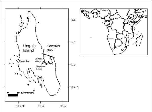
Chwaka Bay is located within 6.13-6.25°S and 39.37-39.58°E on the east coast of Unguja Island, about 34 km east of Zanzibar town. Large intertidal flats partly covered with mixed assemblages of algae and seagrass beds characterize the bay. On the landward side of its mouth, the bay is fringed by a dense mangrove forest, which is drained by a number of tidal creeks, the largest of which is Mapopwe Creek, which is the main water exchange route between the forest and the bay. A modest fragmented coral reef occurs at the entrance of the bay, which is part of the extensive reef that fringes the east of Unguja Island (Figure 2.1).

There are two rain seasons in Zanzibar: the first, during the months of March, April and May, is referred to as long rains, and the second, ‘short rains’, extends from October to December. Therefore

March-May and October-December constitute the wet season in Zanzibar. The months of January-February and June-September constitute the dry season. There are no major rivers that enter directly into the bay, except for some small seasonal streams that flow during rainy seasons. However, there seems to be a significant underground water flow into the bay, but this has not been measured. On the other hand, the bay does not have any significant industrial development. Therefore no effluents or pollutants directly associated with industries find their way into the bay. The estimated population at Chwaka village is about 9,000 people. Untreated sewage is commonly dumped directly into the bays. However, anthropogenic effects may not be an important factor in this bay. Other environmental pollutants such as agro-chemicals are also insignificant.

3 9 .2 ° E 3 9 .4 3 9 .6 6 .4 °S 6 .2 6 .0 5 .8 Unguja Island Ma popw e C reek # # Ch waka Village Z an z ib a r Chw a ka Ba y 0 10 Kil om eters

Chwaka

Bay

Figure 2.1. Map of Chwaka Bay, Zanzibar. Bars on the bay show the budgeted outer and inner

compartments of the bay.

For the purpose of describing the salt, water and nutrient budgets in Chwaka Bay, it is convenient to separate the system into two compartments. The first compartment comprises the inner bay that includes Mapopwe Creek (Figure 2.1). The second compartment comprises the main outer bay, which opens into the open ocean. The two compartments are physically separated by a coral sill near the entrance to the creek, so that water exchange between the two compartments is only through the upper 1 m above the sill. There is also a marked salinity difference between the two compartments. The surface area of the inner system is about 5 km2 with a depth of about 2 m, and total volume of the inner system 10x106 m3. The surface area of the outer system is about 45 km2 with a depth of about 4 m, and total volume 180x106 m3.

Water and salt balance

The concept behind the water budgets is to establish the balance of freshwater inflow (such as runoff, precipitation, groundwater, sewage) and evaporative loss of freshwater. There must be a compensating outflow (or inflow) in order to balance the water volume in the system. Since salt must be conserved in

the system, the salt fluxes accounted for by the salinity used to describe the fresh water advective flows must be balanced by mixing (Gordon et al. 1996).

The data used here were collected in June 1998, just after the end of long rains, and November 1998 during the wet season. Table 2.1 gives a summary of monthly averages of the rainfall for year 1998, and monthly averages of evaporation for Zanzibar. The average rainfall for June was 12 mm d-1 and that for November 17 mm d-1. The average pan evaporation for all seasons were equal, estimated at about 5 mm d-1. However pan observations are known to be affected by a variety of factors: vapor pressure difference, wind, water temperature, pan diameter, air pressure, rim height, pan color, pan depth, pan immersion in the soil and exposure. Evaporation from a pan is usually greater than from larger water bodies because of higher water temperatures. The excess is corrected by a pan coefficient (PC), which is given by:

PC = (evaporation from a free water surface)/(evaporation from a pan)

Table 2.1. Zanzibar mean monthly rainfall and evaporation (1998).

Month Rainfall (mm month-1) Evaporation (mm month-1) January 310 150 February 180 180 March 90 150 April 600 150 May 90 120 June 45 150 July 10 120 August 0 150 September 100 150 October 510 150 November 320 150 December 400 150 Mean 183 150

The correction depends on the size of the pan, e.g. for 4 ft diameter 10 inches deep pans use PC = 0.7 and for 10 ft diameter 24 inches deep pan use PC = 0.95 (William 1997; Nolte and Associates 1998). For this budget, the pan coefficient of 0.7 was applied to convert the measured daily evaporation value of 5 mm d-1 to 3.5 mm d-1, which is the free water surface evaporation value. The obtained free water surface evaporation is also consistent with the value obtained using Hamon's Equation (Hamon 1961) where estimated evaporation of 3.6 mm d-1 was obtained using the temperature data for Zanzibar during the dry season.

The rainfall value of 12 mm d-1 and 17 mm d-1 for June and November respectively and evaporation of 3.5 mm d-1 for both seasons, together with the data on the bay surface area, were used to calculate the precipitation and evaporation water volumes per day in the bay for the dry and wet seasons.

The estimation of the underground water flow (VG) was a problem for this system, because the parameter has not been measured. Therefore the groundwater input was estimated using Darcy’s Law (Shaw 1996). That empirical relationship is given by the following equation:

VG( Approx) = -K[(h2-h1)/d]LW

where K is the hydraulic conductivity given to be 6x10-4 m sec-1 for mainly coralline deposits (Woodward-Clyde 1999); h1 and h2 are the lower and upper hydraulic heads which for inner and outer

bays the difference is estimated to be 2 m (tidal range); d is the watershed, which is 6 km and 2.5 km for the inner and outer bay, respectively; L is the length of the coastline, which is 9.5 km for the inner Bay and 18 km for the outer bay; and W is the width of the flow, which for Chwaka Bay is 2 m. The calculation using this relationship is good for estimation of typical annual groundwater flows only and unrealistic for estimating monthly averages. The same values were therefore applied for quantifying the average groundwater flow for both dry and wet seasons. It is noted however that the values for the wet season could be higher than those during the dry season. The calculations done for this system in the inner and outer bays gave:

VG(Inner Chwaka) = 0.3x10 3 m3 d-1 VG(Outer Chwaka) = 1.5x10 3 m3 d-1

Since the system is separated into two compartments, there are two salinity input values necessary for the calculation of salt balance between the compartments and between the big outer Chwaka Bay and the open ocean. These salinity values are shown in Figure 2.2. The salinity of the inner bay, outer bay and open ocean are indicated as S1, S2 and Socn respectively. Similarly, the volume and surface area of

the inner bay and outer bay are indicated as V1, A1 and V2, A2, respectively.

The water balance for each season is calculated using Equation (1) from Gordon et al. (1996):

dV/dt = VQ + VP + VG + VO + VE +VR (1)

where VQ is rate of river discharge, VP is precipitation, VO is sewage discharge, VE is evaporation and VR is residual flux. Assuming steady state (i.e. dV/dt = 0), then the residual flow is:

VR = VE -VQ –VP –VG –VO (2)

Substituting terms in Equation (2) with data in Table 2.2, the values of VR can be obtained for the wet and dry seasons.

On the other hand, the salt balance is calculated from Equation (3), in order to balance salt input via mixing with salt output from residual outflow. It is assumed that the salinity of out-flowing water (SR) is the average of the salinities between the compartments under consideration [SR=(S1+S2)/2].

dVS/dt = VQSQ + VPSP + VGSG + VOSO + VESE +VRSR + VX (S2 -S1) (3)

where VX represents the mixing volume exchanged between the ocean and the bay, and VRSRis the salt flux carried by the residual flow. The general principle is that salt must be conserved so the residual salt flux is brought back to the system through the mixing salt flux across the boundary [VX (S2 -S1] via the tides, wind and general ocean circulation pattern.

Since the salinity of freshwater inflow terms can be assumed to be 0, then Equation (3) can be simplified to:

dVS/dt = VRSR + VX (S2 -S1) (4)

Assuming that S1 remains constant with time (steady state):

0 = + VRSR + VX (S2 -S1) (5)

By re-arrangement:

Substituting terms in Equation (6) with salinity data, the mixing volume (VX) for different compartments can be obtained as illustrated in Figure 2.2 for the wet and dry seasons.

The water exchange or freshwater residence time (τ) in days for both wet and dry seasons can be calculated from Equation 8, where |VR| is the absolute value of VR:

τ = Vsyst /(VX + |VR|) (8)

Vsyst is the total volume of the bay or in our case the volume of the individual compartments. Figure 2.2 summarizes the water and salt flux for this two-box system and gives the water exchange time based on the data.

Chwaka Bay water and salt balance has demonstrated that in order to balance the inflow and outflow of water for June, there must be a net flux of water from the bay to the open ocean (VR = -42x10

3

m3 d-1 for inner bay and VR = -426x10

3

m3 d-1 for outer bay). Similarly, there is a net flux of water from the bay to the ocean during November (VR = -67x10

3

m3 d-1 for inner bay and VR = -676x10

3

m3 d-1 for outer bay). The corresponding residual fluxes of salt (VRSR) from the two boxes indicate advective salt export. However, the exchange of bay water with the open ocean plays a role of replacing this exported salt via mixing (VX). In this data, the total exchange times (flushing time or freshwater residence time) were 20 and 22 days for the inner and outer bays, respectively for the month of June, and 5 and 26 days for the inner and outer bays respectively for the month of November. Water exchange time of the entire bay with the open ocean is 24 days in June and 37 days in November.

The mixing volumes were estimated from mixing equations in a 1-dimensional, steady state system (Yanagi 2000a) for comparison with the results obtained using water and salt balance method. The estimated mixing using Yanagi's method gave VX1 = 1,200x10

3

m3 d-1 and VX2 = 4,000x10

3

m3 d-1 for the inner and outer bay, respectively. These values were consistent with the VX obtained from the salt and water balance for both June and November.

This budget has demonstrated that it is difficult to obtain realistic budgets for systems that are dominated by evaporation that is almost comparable with net precipitation in the absence of runoff. It also showed that unrealistic budgets could be obtained by using the pan evaporation data. It is always important to convert the pan evaporation values to free water surface evaporation values. The use of pan coefficients ranging from 0.6-0.8 is recommended, depending on the size of the pans used. In this example, a pan coefficient of 0.7 was applied and provided realistic water and salt budgets for this system. It was also found that, in order to obtain realistic budgets, it is useful to compare the VX values obtained from salt-water balance with those obtained using Yanagi's method. The experience from this budget also showed that budgets for different seasons could be significantly different. It is therefore important to specify the seasons and preferably the month when the data used in budgets were taken. Budgets for nonconservative materials

The nutrient data were only available for the month of November. The discussion in this section is therefore limited to the wet season. The general principle is that all the dissolved inorganic phosphorus (DIP) and dissolved inorganic nitrogen (DIN) will exchange between the system and the adjacent ocean according to the criteria established in the water and salt budget. Deviations are attributed to net nonconservative reactions of (DIP) and (DIN) in the system. DIP is defined as the PO4 concentration

and DIN as the (NO3

+ NO2

+ NH4+). The data from Chwaka Bay show the concentration of DIP in the inner and outer bay to be DIP1 = 2.0 ìM and DIP2 = 1.2 ìM, respectively (Figure 2.3). Likewise,

the concentration of DIN in the inner and outer bay are DIN1 = 23 ìM and DIN2 = 18 ìM, respectively

(Figure 2.4). Following Wyrtki (1971) the concentration of DIN and DIP in the open ocean (Zanzibar Channel) are DIPocn = 0.1 ìM and DINocn = 0.5 ìM, respectively.

This system poses a challenge for estimating fluxes of nutrients because the groundwater nutrient and nutrient loading associated with waste discharge concentration are unknown. The V DIP and V DIN

were assumed to be zero since Chwaka Bay has no rivers. The VatmDIPatm and VatmDINatm were assumed

to be zero because atmospheric contribution is normally very small. However, although the population around Chwaka Bay is fairly small (9,000 people), the anthropogenic effects (VODIPO, VODINO) were considered here because the initial estimates of ÄDIPand ÄDINwere relatively small. The waste load from solid waste, domestic waste and detergents could therefore be important for this system and were estimated using a method suggested by McGlone et al. (1999). Since the waste is dumped directly to the bay, it was assumed that 100% of the waste load does actually reach the bay waters. The values of VODIPO = 900 mol d

-1

and VODINO = 4,000 mol d

-1

were obtained and used in the calculation of the budget for this system. Note that the waste load for the inner bay was taken to be zero because only the areas around the outer bay are inhabited.

Similarly, although the DIPG flux in groundwater flowing through carbonate terrain is known to be low,

the concentration of nitrogen (DING) in the underground water could not be neglected. For the nutrient

calculations reported here, DIPG concentrations of 0.4 ìM and 2 ìM were used for the inner (DIPG1)

and outer (DIPG2) systems, respectively. These values are comparable to reported groundwater PO4 for

similar systems (1-10 ìM: Lewis 1985; Tribble and Hunt 1996). Similarly, DING concentrations of 25

ìM and 37 ìM were used for the inner (DING1) and outer (DING2) systems, respectively.

DIP and DIN balance

DIP and DIN budget results for nonconservative materials in Chwaka Bay are illustrated in Figures 2.3 and 2.4. The calculated ÄDIP1and ÄDIP2for the wet season are +1,700 mol d

-1

(+0.3 mmol m-2 d-1) and +2,600 mol d-1 (+0.06 mmol m-2 d-1), respectively, indicating that there is a net DIP flux from the bay to the ocean for the month of November (i.e. ÄDIP is positive). The calculated ÄDIPsyst = +4,300 mol d-1 or +0.1 mmol m-2 d-1. Chwaka Bay acts as a DIP source during the wet season.

The calculated ÄDIN1 and ÄDIN2 for the wet season are +11,000 mol d

-1

(+2.2 mmol m-2 d-1) and +68,000 mol d-1(+1.5 mmol m-2 d-1), respectively, indicating that there is a net DIN flux from the bay to the ocean during the wet season (i.e. ÄDIN is positive). The calculated ÄDINsyst = +79,000 mol d

-1

(+1.6 mmol m-2 d-1). Thus as for DIP, Chwaka Bay is a net source of DIN during the wet season.

Stoichiometric calculations of aspects of net system metabolism

In general, the LOICZ Biogeochemical Modelling Guidelines (Gordon et al. 1996) were used to calculate the stoichiometrically linked water and salt-nutrients budgets. In these mass balance budgets, complete mixing of the water column is assumed. The general principle is that the nonconservative flux of DIP with respect to salt and water is an approximation of net ecosystem metabolism (production-respiration, p-r) at the scale of the system. The net ecosystem metabolism can be calculated from ÄDIP. Thebasic formulation is as follows:

(p-r) = -ÄDIP x (C:P)part

where (C:P)part represents the C:P ratio of organic matter that is reacting in the system, which is

expected to be near 106:1. On the other hand the nonconservative flux of DIN approximates net nitrogen fixation and denitrification in the system. The basic formulation is as follows:

(nfix-denit) = ÄDIN - ÄDIP(N:P)part

where (N:P)partrepresents the ratio of both planktonic and waste derived organic matter reacting in the

system, which is expected to be near 16:1. Table 2.2 shows the stoichiometric calculations made for Chwaka Bay for November 1998.

Because of unavailability of monthly nutrient data for the whole of 1997, the results from Chwaka Bay could not clearly demonstrate the dependence of seasonality in the nutrient budget. Stoichiometric calculations suggest that (p-r) is negative (Table 2.2) for all three regimes (inner, outer and entire bay).

This indicates that Chwaka Bay is net heterotrophic during the wet season. Chwaka Bay seems to have net denitrification in the inner bay as indicated by the negative (nfix-denit)value and the outer bay to be net nitrogen-fixing at a slower rate (Table 2.2). However, the entire bay seems to balance nitrogen fixing and denitrification, since (nfix-denit) for the entire bay is zero.

Table 2.2. Summary of calculated (p-r) and (nfix-denit) values for Chwaka Bay for November

1998 (wet season).

Calculated Values Inner Chwaka Bay Outer Chwaka Bay Entire bay

ÄDIP (mol d-1) +1,700 +2,600 +4,300 ÄDIP (mmol m-2 d-1) +0.3 +0.06 +0.1 ÄDIN (mol d-1) +11,000 +68,000 +79,000 ÄDIN (mmol m-2 d-1) +2.2 +1.5 +1.6 (p-r) (mmol C m-2 d-1) -32 -6 -11 (nfix-denit) (mmol N m-2 d-1) -2.6 +0.5 0

Figure 2.2. Water and salt balance for Chwaka Bay for June 1998 (a) and November 1998 (b).

Water flux in 103 m3 d-1 and salt flux in 103 psu-m3 d-1. Inner Chwaka V1 = 10 x 10 m A1 = 5 x 10 m S1 = 31 psu τ1 = 20 days VX1(S2-S1) = -VR1SR1 = 1,365 VX1 = 455 VG1 = 0.3 Socn = 36 ττsyst = 24 days VP1 = 60 VE1 = 18 VR2 = 426 VR1 = 42 Outer Chwaka V2 = 180 x 10 m A2 = 45 x 10 m S2 = 34 psu τ2 =22 days VP2 = 540 VE2 = 158 6 3 6 2 2 3 6 6 VG2 = 1.5 a) June VX2(SOcn-S2) = -VR2SR2 = 14,910 VX2 = 7,455 VO1 = 0 VX1(S2-S1) = -VR1SR1 =1,977 VX1 _{= 1,977} Inner Chwaka V1 = 10 x 10 m A1 = 5 x 10 m S1 = 29 psu τ1 = 5 days VG1 = 0.3 Socn = 35 ττsyst = 37 days VP1 = 85 VE1 = 18 VR2 =676 VR1 = 67 Outer Chwaka V2 = 180 x 10 m A2 = 45 x 10 m S2 = 30 psu τ2 = 26 days VP2 = 765 VE2 = 158 6 3 6 2 2 3 6 6 VG2 = 1.5 VX2(Socn-S2) = -V2SR2 =21,970 VX2 _{= 4,394} b) November VO1 = 0

Figure 2.3. DIP budget for Chwaka Bay for November 1998 (wet season). Flux in mol d-1 and concentration in ìM or mmol m-3.

Figure 2.4. DIN budget for Chwaka Bay for November 1998 (wet season). Flux in mol d-1 and

concentration in ìM or mmol m-3. Outer Chwaka DIP2 = 1.2 µM ∆ ∆DIP = +2,600 VG!DIPG1 = 0.1 VR2DIPR2 = 400 DIPocn = 0.1

VX2(DIPocn-DIP2) = 4,800 Inner Chwaka DIP1 = 2.0 µM ∆ ∆DIP = +1,700 VX1(DIP2 - DIP1) = 1,600 VR1DIPR1 = 100 VO1DIPO1 = 0 ∆ ∆DIPsyst = +4,300 November VO2DIPO2 = 900 VG2DIPG2 = 3 Outer Chwaka DIN2 = 18 µM ∆ ∆DIN = +68,000 VG!DING1 = 8 _VR2DINR2 = 6,000 DINocn = 0.5

VX2(DINocn-DIN2) = 77,000 Inner Chwaka DIN1 = 23 µM ∆ ∆DIN = +11,000 VX1(DNP2 - DIN1) = 10,000 VR1DINR1 = 1,000 VO1DINO1 = 0 ∆ ∆DINsyst _{= +79,000} November VO2DINO2 = 4,000 VG2DING2 = 60

2.2 Makoba Bay, Zanzibar

A.S. Ngusaru and A.J. Mmochi

Study area description

Makoba Bay is located within 5.90-5.95°S and 39.20-39.25°E on the northwest coast of Unguja Island, Zanzibar (Figure 2.5). It is sheltered by the much smaller Tumbatu Island, which is located about 5 km offshore to the north. The bay has a total surface area of about 15 km2 and average depth of 5 m with a volume of about 75x106 m3. The tides in Makoba Bay are mainly semi-diurnal with a typical tidal range of about 2 m. Local climate is characterized by two rainy seasons: the long rains occur in March, April and May and the short rains during October, November and December. Therefore March-May and October-December constitute the wet season in Zanzibar. January-February and June-September constitute the dry season in Zanzibar. The estimated population around the bay is about 10,000 people. Untreated sewage is usually dumped directly into the bay. Industrial and agro-chemicals are also commonly applied, and the runoff from these also flows into the bay.

Figure 2.5. Map and location of Makoba Bay, Zanzibar. The bar at the mouth of the bay shows the

budgeted area.

Water and salt balance

The basic principle for the water and salt budgets is to establish balance of freshwater inflow (such as runoff, precipitation, groundwater, sewage) and evaporative loss. Then compensating outflow (or inflow) is calculated to balance the water volume in the system. Since salt must be conserved in the system, the salt fluxes accounted for by the salinity used to describe the freshwater flows must be balanced by mixing (Gordon et al. 1996). Makoba Bay is the largest water catchment area in Zanzibar,

Zanzibar Makoba Bay Unguja Island Makoba Bay 39.2°E 39.4 5.8. 5.9°S 6.0 Makoba Bay Unguja Island Kipange R. Mwanakombo R. Zingwezingwe R. Tumbatu Island Indian Ocean 5 km

referred to as the Mahonda-Makoba drainage basin. It drains rice farms, sugar cane plantations, a sugar factory and a rubber factory. Three main rivers with multiple rivulets provide a substantial amount of freshwater input directly to the bay, namely the Mwanakombo, Zingwezingwe and Kipange rivers. These rivers have a total watershed area of 150 km2 with a total mean discharge of 24x106 m3 yr-1 or about 70x103 m3 d-1.

The data used for this budget were collected in April 1997, during the wet season in the area. Table 2.3 shows the monthly rainfall data for 1997; the average rainfall of 14 mm d-1 was used in this budget. Mean pan evaporation rate is 5 mm d-1, however pan observations are commonly affected by such factors as vapor pressure difference, wind, water temperature, pan diameter, air pressure, rim height, pan color, pan depth, pan immersion in the soil and exposure. Evaporation from a pan is usually greater than from larger water bodies because of higher water temperatures. The excess is corrected by a pan coefficient (PC), which is given by:

PC = (evaporation from a free water surface)/(evaporation from a pan)

The correction depends on the size of the pan, e.g. for 4 ft diameter 10 inches deep pans use PC = 0.7 and for 10 ft diameter 24 inches deep pan use PC = 0.95 (William 1997; Nolte and Associates 1998). For this budget, the pan coefficient of 0.7 was applied to convert the measured daily evaporation value of 5 mm d-1 to 3.5 mm d-1, which is the free water surface evaporation value. The obtained free water surface evaporation is also consistent with the value obtained using Hamon's equation (Hamon 1961) where estimated evaporation of 3.6 mm d-1 was obtained using the temperature data for Zanzibar.

Table 2.3. Zanzibar mean monthly rainfall and evaporation (1997).

Month Rainfall (mm) Evaporation

(mm) January 0 150 February 50 180 March 425 150 April 310 150 May 250 120 June 215 150 July 40 120 August 40 150 September 0 150 October 510 150 November 315 150 December 45 150 Mean 183 221

The rainfall value of 14 mm d-1 and evaporation of 3.5 mm d-1 together with the data on the bay surface area were used to calculate the precipitation and evaporation water volume per day in the bay for the dry season as shown in Figure 2.6.

Unfortunately the underground water flow (VG) was not measured. The groundwater input was therefore estimated using Darcy’s Law (Shaw 1996). The empirical relationship is given by the following equation:

VG( Approx) = -K[(h2-h1)/d]LW

Where K is the hydraulic conductivity given to be 6x10-4 m sec-1 for mainly coralline deposits (Woodward-Clyde 1999); h1 and h2 are the lower and upper hydraulic heads which for inner and outer

bays the difference is estimated to be 2 m (tidal range); d is the watershed which is 15 km; L is the length of the coastline, which is about 20 km and W is the width of the flow, which for Makoba Bay is about 2 m. The calculation using this relationship is good for estimation of typical annual ground water flows only and unrealistic for estimating monthly averages. The same obtained values were therefore used for quantifying the average groundwater flow for both dry and wet seasons. However, the values for the wet season should be higher that those during the dry season. The calculations done for Makoba Bay gave:

VG = 0.3 x 10 3

m3 d-1

The salinity-input values for the calculation of salt balance between Makoba Bay and the open ocean are shown in Figure 2.6. The salinity of the bay and open ocean is indicated as Ssyst and Socn,

respectively. Similarly, the volume and surface area of the bay are indicated as Vsyst and Asyst

respectively.

The water balance for each season is calculated using Equation (1) from Gordon et al. (1996):

dV/dt = VQ + VP + VG + VO + VE +VR (1)

where VQ is rate of river discharge, VP is precipitation, VO is sewage discharge, VE is evaporation and VR is residual flux. Assuming steady state (i.e. dV/dt = 0), then the residual flow is:

VR = VE -VQ –VP –VG –VO (2)

Substituting terms in Equation (2) with data in Table 2.3, the values of VR can be obtained for the wet and dry seasons.

On the other hand, the salt balance is calculated from Equation (3), in order to balance salt input via mixing with salt output from residual outflow. It is assumed that the salinity of out-flowing water (SR) is the average of the salinities between the bay and open ocean.

[SR=(Ssyst+Socn)/2].

dVS/dt = VQSQ + VPSP + VGSG + VOSO + VESE +VRSR + VX (Socn –Ssyst) (3)

where VX represents the mixing volume exchanged between the bay and the ocean, and VRSRis the salt flux carried by the residual flow. The general principle is that salt must be conserved so the residual salt flux is brought back to the system through the mixing salt flux across the boundary [VX (Socn - Ssyst] via the tides, wind and general ocean circulation pattern.

Since the salinity of freshwater inflow terms can be assumed to be 0, then Equation (3) can be simplified to:

dVS/dt = VRSR + VX (Socn - Ssyst) (4)

Assuming that Ssyst remains constant with time (steady state):

0 = + VRSR + VX (Socn - Ssyst) (5)

By re-arrangement:

VX = -VRSR /(Socn - Ssyst) (6)

Substituting terms in Equation (6) with salinity data, the mixing volume (VX) can be obtained as illustrated Figure 2.6 for both wet and dry seasons.

The water exchange or freshwater residence time (τ) in days for both wet and dry seasons can be calculated from Equation 8, where |VR| is the absolute value of VR:

τ = Vsyst /(VX + |VR|) (8)

Figure 2.6 summarizes the water and salt flux for this system and gives the water exchange time based on the data. The Makoba Bay water and salt balance has demonstrated that in order to balance the inflow and outflow of water during the wet season there is net flux of water from the bay to the open ocean (VR = -223x10

3

m3 d-1). The residual fluxes of salt (VRSR) between the bay and the open ocean indicate advective salt export; the exchange of bay water with the open ocean plays a role of replacing this exported salt via mixing. The calculated water exchange time (flushing time or freshwater residence time) for Makoba Bay is 63 days during the wet season.

Budgets of nonconservative materials

The dissolved inorganic phosphorus (DIP) and dissolved inorganic nitrogen (DIN) budgets are termed the budgets of nonconservative materials. While this might be done with any reactive material, the particular interest here is in the balance among the essential elements C, N, and P. The general principle behind the budgets is that the DIP and DIN will exchange between the system and the adjacent ocean according to the criteria established in the water and salt budgets. Deviations are attributed to net nonconservative reactions of DIP and DIN in the system. DIP is defined as the PO4

-3

concentration and DIN as the (NO3

+ NO2

+ NH4+).

Due to limited data, the discussion of nutrient budgets for Makoba Bay is limited to the wet season only. The data from Makoba Bay show the concentration of DIP in the bay to be DIPsyst = 0.2 µM

during the wet season (Figure 2.7). Likewise, the concentration of DIN in the bay is DINsyst = 32 µM

for the wet season (Figure 2.8). Following Wyrtki (1971) the concentration of DIN and DIP in the open ocean (Zanzibar Channel) are DIPocn = 0.1 µM and DINocn = 0.5 µM. The concentrations in the rivers

were estimated at DIPQ = 0.3 µM and DINQ = 6 µM.

This system poses a challenge for estimating fluxes of nutrients because the groundwater nutrient and nutrient loading associated with waste discharge concentration are unknown. The DIPatm and DINatm

were assumed to be zero because atmospheric contribution is normally small. The population around Makoba Bay is fairly small (10,000 people); nevertheless the waste load from solid waste, domestic waste and detergents were estimated using a method suggested by McGlone et al (1999). Since the waste is dumped directly to the bay, it was assumed that 100% of the waste load does actually reach the bay waters. The values of VODIPO = 1,100 mol d

-1

and VODINO = 4,400 mol d

-1

were obtained and used in the calculation for the budget. Because of lack of data, the DIP and DIN contributions from agricultural and industrial activities were not included in the budget. Although the DIPG flux in

groundwater flowing through carbonate terrain is known to be low, the concentration of nitrogen (DING) in the underground water could not be neglected. For the nutrient calculations reported here,

DIPG concentration of 2 µM and DING concentration of 37 µM were used. These values are

comparable to reported groundwater PO4 for similar systems (DING = 1-10 µM; DIPG = 37-72 µM:

Lewis 1985; Tribble and Hunt 1996). DIP and DIN balance

The budget results for nonconservative materials in Makoba Bay are illustrated in Figures 2.6 and 2.7. The calculated ∆DIPand ∆DIN for the wet season is –990 mol d-1 and +29,400 mol d-1, respectively, indicating that there is a net DIP flux from the ocean to the bay during the wet season. Therefore Makoba Bay acts as a sink for dissolved inorganic phosphorus during wet season (∆DIP is negative). There is also a net DIN flux from the bay to the open ocean during the wet season. Makoba Bay is therefore a source of dissolved inorganic nitrogen (∆DIN is positive) during the wet season.

Stoichiometric calculations of aspects of net system metabolism

The LOICZ Biogeochemical Modelling Guidelines (Gordon et al. 1996) were used to calculate the stoichiometrically linked water-salt-nutrients budgets. In these mass balance budgets, complete mixing of the water column is assumed. The general principle is that the nonconservative flux of DIP with respect to salt and water is an approximation of net ecosystem metabolism (production-respiration, p-r) at the scale of the system in question. The net ecosystem metabolism can therefore be calculated from

∆DIP using the following basic formulation, (p-r) = -∆DIP x (C:P)part

where (C:P)part represents the C:P ratio of organic matter that is reacting in the system, which is

expected to be near 106:1.

On the other hand the nonconservative flux of DIN approximates net nitrogen fixation and denitrification in the system. The basic formulation is as follows:

(nfix-denit) = ∆DIN - ∆DIP(N:P)part

where (N:P)partrepresents the ratio of both planktonic and waste-derived organic matter reacting in the

system, which is expected to be near 16:1. Table 2.4 shows the stoichiometric calculations made for Makoba Bay.

Stoichiometric calculations suggest that (p-r) is positive during the wet season (Table 2.4). This indicates that Makoba Bay is net autotrophic during the wet season. Makoba Bay is fixing nitrogen during wet season, where (nfix-denit)is estimated to be 3 mmol m-2 d-1 in excess of denitrification. The summary of fluxes of nonconservative nutrients in Makoba Bay is given in Table 2.4. Nitrogen fixation is known to provide the nitrogen requirement in areas dominated by seagrass beds and mangroves (Hanisak 1993). The occurrence of mangroves and seagrass beds at Makoba Bay is a possible ecological reason behind the balance of nitrogen fixation over denitrification in the bay.

Table 2.4. Summary of calculateded (p-r) and (nfix-denit) values for Makoba Bay for April 1997

(wet season).

Parameters Calculated values

∆ ∆DIP (mol d-1) -990 ∆ ∆DIP (mmol m-2 d-1) -0.07 ∆ ∆DIN (mol d-1) +29,400 ∆ ∆DIN (mmol m-2 d-1) +2 (p-r) (mmol C m-2 d-1) +7 (nfix-denit) (mmol N m-2 d-1) +3

Figure 2.6 Water and salt balance for Makoba Bay for April 1997 (wet season). Water flux in 103 m3 d-1 and salt flux in 103 psu-m3 d-1.

Figure 2.7. DIP budget for Makoba Bay for April 1997 (wet season). Flux is in mol d-1 and

concentration in µM or mmole m-3.

Figure 2.8. DIN budget for Makoba Bay for April 1997 (wet season). Flux is in mol d-1 and

concentration in µM or mmole m-3. Makoba Bay Vsyst = 75 x 10 m Asyst = 15 x 10 m Ssyst = 27 psu τ τ = 63 days VP = 210 VE = 53 VQ = 66 VR = 223 VX(Socn-Ssyst) = -VRSR = 6,802 VX = 972 6 3 VG = 0.3 6 2 Socn = 34 psu SR = 30.5 psu April 1997 Makoba Bay DIPsyst = 0.2 µM ∆ ∆ DIPsyst = -990 DIPQ = 0.3 µM VQDIPQ = 20 VRDIPR = 30 DIPocn = 0.1 µM DIPR = 0.15 µM

VX(DIPocn-DIPsyst) = 100

VatmDIPatm =0 April 1997 DIPG = 0.2 µM VGDIPG = 0 VODIPO = 1,100 Makoba Bay DINsyst = 32 µM ∆ ∆ DINsyst = +29,400 DINQ = 6 µM VQDINQ = 400 VRDINR = 3,600 DINocn = 0.5 µM DINR = 16.25 µM

VX(DINocn-DINsyst)

= 30,600

VatmDINatm =0 April 1997

DING = 37 µM VGDING = 0

2.3 Malindi Bay, Kenya

Mwakio P. Tole

Study area description

Malindi Bay, towards the south coast of Kenya, is semi-enclosed to the north and to the south, but open to the ocean over a patchy coral reef ecosystem. Sea grasses and algae are common in southern and northern ends of the bay. A small mangrove forest occurs on the banks of the Sabaki River about 1 km from the ocean. Figure 2.9 shows the location of the study area. The area is estimated to be 18 km2. Mean annual rainfall in the Malindi Bay area, and for most of the drainage basin, is 972 mm per annum, and ranges from 677mm during dry years to 1267mm during wetter years. Annual evaporation is much higher than the rainfall, at 1800 mm per year. Temperatures range from 28°±7°C at Malindi in the coast, to 20°±7°C in the highland areas around Nairobi.

The Athi-Galana-Sabaki River system rises from the highlands in the central part of the country, and is the second largest river draining into the Indian Ocean in Kenya. It has a length of 400 km, and drains a basin area of 70,000 square kilometers It enters the Indian Ocean at 3.2o S 40.15oE, just north of Malindi town (population approximately 50,000) in Malindi Bay. The Sabaki River flow rate ranges from a low of 0.52 m3 s-1 in the driest periods, to 758 m3 s-1 during times of flood. Mean flow rate was 48.8 m3 s-1 over the period 1957 to 1979.

Industrial and municipal wastes from Nairobi City (population approximately 2 million) drain into the river, sometimes with little treatment. The river also receives agrochemicals (fertilizers, pesticides) from farms that grow coffee, tea, horticultural crops (including cut flowers), and from maize farming. Dairy and beef farming is also practised along the river basin.

S a b a k i R iv e r M alin di B ay M a li n d i T o w n Indi an O ce an 3. 1 3. 2 ° S 40 . 1° E 40 . 2 0 2 K il o m e t e rs M al in d i B ay

Mean annual rainfall in the Malindi Bay region is 1,000 mm, and ranges from 700 mm during dry years to 1,300 mm during wet years. Annual evaporation is 1,800 mm.

The Sabaki River flow rate ranges from 0.5 m3 s-1 (40x103 m3 d-1) in the driest periods to 760 m3 s-1 (70x106 m3 d-1) during times of flood. Mean flow rate was 50 m3 s-1 (4x106 m3 d-1)over the period 1957 to 1979. Malindi Town has a population of approximately 50,000 people. Water abstracted upstream in the Sabaki River is used in the town, and becomes wastewater that is assumed discharged directly into the Malindi Bay. The volume of this has been estimated to be 20x103 m3 d-1.

Tidal influence is high in Malindi Bay, with tidal ranges between 2 and 3 m. Waves, particularly during the SE monsoon period (April–September), range up to 2 m near the shore. The mean depth of the bay is 2 m. The system is well-flushed and fairly well-mixed.

Water and salt balance

The water and salt budgets describe the exchange of water and salt between the Malindi Bay and the Indian Ocean (Figure 2.10). Freshwater inputs are from the Sabaki River (VQ), precipitation (VP) and Malindi Town sewage (VO), while loss is to the open ocean (VR) and by evaporation (VE). Salt must be conserved in the system, hence salt flux out from the system carried by the residual flow (VR) must be balanced via mixing (VX). There are two distinct wet seasons and two dry seasons each of about three months. Data were collected in 1997 and 1998, and were affected by unusually heavy El Nino rains, so that the dry seasons were masked by flooding rains. There were no distinct dry seasons during the El Nino rains in 1997-1998. Tables 2.5 and 2.6 indicate the data used to compile the water and salt budgets.

Table 2.5. Malindi Bay water fluxes (in 106 m3 d-1) and water exchange time (ττ).

Oct–Dec (wet) Jan–Mar (dry) Apr–Jun (wet) Jul–Sep (dry) Annual Surface runoff (VQ) 6 5 5 5 5 Groundwater (VG) 0 0 0 0 0 Precipitation (VP) 0 0. 0 0 0 Evaporation (VE) 0 0 0 0 0 Outfall (VO) 0 0 0 0 0 Residual flow (VR) 6 5 5 5 5 Mixing (VX) 11 9 8 9 9 τ τ (days) 2 3 3 3 3

The water balance for each season is calculated based on Gordon et al. (1996). Precipitation, evaporation and sewage flow were considered insignificant compared to high river flow. Water fluxes and water exchange time (τ) are summarized in Table 2.5. The water exchange time, based on the average data, was 2 to 3 days.

Balance of nonconservative materials

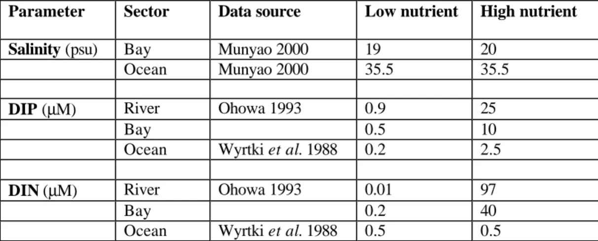
Available data for nutrient concentrations used in this budget were measured in different years. Nutrient concentrations for Sabaki River were taken from Ohowa 1993, Giesen and Kerkhof 1984, and Heip et al. 1995; and oceanic concentrations from Wyrtki et al. 1988 (see Table 2.6). The nutrient concentrations measured in those years vary significantly between dry and wet seasons with low concentrations during the dry seasons and high during the wet seasons. Nonconservative budgets were developed for the low and high nutrient concentrations using annual average water budget for 1997-1998 (Figure 2.10).

Table 2.6. Salinity and nutrient concentrations for Sabaki River, Malindi Bay and adjacent ocean.

Parameter Sector Data source Low nutrient High nutrient

Salinity (psu) Bay Munyao 2000 19 20

Ocean Munyao 2000 35.5 35.5

DIP (µM) River Ohowa 1993 0.9 25

Bay 0.5 10

Ocean Wyrtki et al. 1988 0.2 2.5

DIN (µM) River Ohowa 1993 0.01 97

Bay 0.2 40

Ocean Wyrtki et al. 1988 0.5 0.5

Estimated loads from all sources - domestic, hotels, storm runoff, solid wastes, industrial waste, agricultural waste, and livestock waste (modified after Munga et al. 1993) are 34 tonnes per annum of phosphorus and 168 tonnes per annum of nitrogen. These exclude what is inputted into the ocean through the Sabaki River. The estimated loads were converted to dissolved inorganic phosphorus (DIP) and dissolved inorganic nitrogen (DIN) using DIP:TP (0.5) and DIN:TN (0.4) in San Diego-McGlone et al. 1999 with the assumption that 100% of the estimated nutrient loads enter the bay.

Table 2.7 summarizes the fluxes of DIP and DIN for Malindi Bay. The system appears to be a net sink for both DIP and DIN. However, there is a large amount of uncertainty in these budgets because of the extreme range in estimated nutrient concentrations.

Table 2.7. Summary of nutrient fluxes and stoichiometically derived (p-r) and (nfix-denit) for

Malindi Bay, comparing results using the low and high nutrient concentrations data.

Fluxes Low nutrient High nutrient Average

VQDIPQ (103 mol d-1) 5 125 65 VODIPO (103 mol d-1) 2 2 2 VRDIPR (103 mol d-1) -2 -31 -17 VX(DIPocn-DIPsyst) (103 mol d-1) -3 -68 -36 ∆ ∆DIP (103 mol d-1) -2 -28 -15 ∆ ∆DIP (mmol m-2 d-1) -0.1 -1.6 -0.9 VQDINQ (103 mol d-1) 0 485 243 VODINO (103 mol d-1) 13 13 13 VRDINR (103 mol d-1) -2 -101 -52 VX(DINocn-DINsyst) (103 mol d-1) 3 -356 180 ∆ ∆DIN (103 mol d-1) -14 -41 -28 ∆ ∆DIN (mmol m-2 d-1) -0.8 -2.3 -1.6 (p-r)plankton (mmol m-2 d-1) +11 +170 +91 (nfix-denit)plankton (mmol m-2 d-1) +0.8 +23 +12

Stoichiometric calculations of aspects of net system metabolism

Net metabolism of the bay was stoichiometrically derived from the calculated nonconservative DIN and DIP. Assuming that the bay is primarily driven by phytoplankton and using C:N:P ratio of 106:16:1 for phytoplankton, the bay seems to be net autotrophic and fixing nitrogen. The average (p-r) is +91 mmol m-2 d-1 and (nfix-denit) is +12 mmol m-2 d-1 (Table 2.7).

Figure 2.10. Water and salt budgets for Malindi Bay for 1997-1998. Water flux in 106 m3 d-1 and salt flux in 106 psu-m3 d-1.

Malindi Vsyst = 36 x 10 m Asyst = 18 x 10 m Ssyst = 20 psu τ τ = 3 days VP = 0 VE = 0 VQ = 5 VR = 5 Socn = 35.5 psu SR = 27.75 psu VX(Socn-Ssyst) = -VRSR = 139 VX = 9 6 3 VG = 0 6 2 Annual

3. CAMEROON AND CONGO ESTUARINE SYSTEMS Cameroon’s coastal zone and estuarine systems

Cameroon (8-16°E; 2-13°N) is situated on the extreme north-eastern end of the Gulf of Guinea with a surface area of 469,440 km². The main topographical regions are: the low coastal plain covered by equatorial rain forests in the south, the mountain forests peaking at the active Mount Cameroon (4,070 m) in the west, the transitional plateau rising to the Adamaoua Mountains in the centre, and rolling savannah slopes gradating down to the marshlands surrounding Lake Tchad to the north of the Adamaoua Mountain range. Cameroon is drained by four major drainage basins: Atlantic, Zaire/Congo, Niger and Tchad. A watershed exists along the southern Cameroon plateau separating the coastal from the Congo system, with freshwater input into the Atlantic drainage basin.

Cameroon’s coastal zone (Figure 3.1), extends along 402 km (Sayer et al. 1992), from latitude 2.30°N at the Equatorial Guinea borders to 4.67°N at the Nigeria borders. The coastal zone area is estimated at 9,670 km² (Adam 1998) representing 22% of the Gulf of Guinea countries.

Figure 3.1. Cameroon and the Gulf of Guinea.

Cameroon’s coastal climate is of an equatorial type and is influenced by the meteorological equator, being the meeting point between the anticyclone of Azores (North Atlantic) and that of Saint Helen (South Atlantic). This climate results from the combined effect of convergence of the tropical oceanic low-pressure zone and the inter-tropical front within the continent. There are two distinct seasons: a long rainy season of more than 8 months (March-October) and a dry season of four months

(November-February) exist. Air temperatures are high throughout the year. South-westerly monsoon winds predominate, modified by land sea breezes causing humidity values to almost saturation point. Wind speeds exceptionally reach values of 18 m sec-1 (April, 1993) with average values recorded over a period of 10 years (1983 – 1993) varying between 0.5-2.5 m sec-1. The rainy season is hot and dry with a north-easterly harmattan when the inter tropical convergence zone deviates from its normally southern position at 5-7°N.

Cameroon’s coastal tropical rainforest is interrupted at the active Cameroon Mountain and within the mangrove estuarine complexes. These complexes are characterized by very low altitudes (0-20 m), developed on low soils (generally less than 5 m high) with primary stages of mangroves developed at 0-5 m while mature ones reach 2 m. Mangrove estuarine complexes in Cameroon occupy approximately 30% (3,500 km2) of Cameroon’s coastal zone. There are about 38 species of mangrove, dominated by Rhizophora (R. racemosa and R.harrisanii) species (Gabche 1997). This is followed by the Atlantic forest dominated by families of Caesalpinacea and Guttiferae, Euphorbiaceae; swamp forest dominated by Rapphia spp., Matritia quadricorius, Clenolephon englerianus, and seasonally inundated forests of Guitbortia demeussei and Oxysttigma menil. Phytoplankton species (Folack 1991) are dominated by diatoms such as Chaetoceros testissimus, Nitzchia closterium, Diatoma vulgare, Trachyneis and Coscinodiscus.

Dense river networks flow into three estuarine systems along the coast. The West/Rio-del-Rey system has several rivers (Cross, Ndian and Meme) that discharge at the Rio-del-Rey Point (4.8°N; 8.3°E). The Cameroon estuary complex with several rivers (Mungo, Wouri, Dibamba etc) discharges at Douala Point (3.8–4.1°N and 9.25–10°E). This extends towards the west at Bimbia and south to the Sanaga River estuary. The third estuary complex in the south is made up of several rivers (Nyong, Lokoundje, Kienke, Lobe and Ntem) which discharge independently into the Atlantic Ocean. Some physical characteristics of the Cameroon and Rio-del-Rey estuarine complexes are given in Table 3.1. The rivers of these estuaries have watersheds from high altitudes (2,000–2,500 m) at the Adamawa plateau, Rumpi Hills and Manegumba Mountains. The mangroves of the Rio-del-Rey cover an area of about 1,500 km2 with 50 km of coastline and a landward extension of 30 km. The Cameroon estuary has a coastline of 60 km from the Sanaga to the Bimbia estuary and 30 km into the hinterlands giving area of 1,800 km2. The southern river systems at the Ntem also has estuarine mangrove swamps. The supplies from the dense river network, groundwater and rainfall are major sources of freshwater into the continental shelf (area = 15,400 km² ) (Gabche and Folack 1997). The gradual descent (10, 30, 50 and 100 m depth) of the continental shelf results in generally weak circulation with subsequent high sedimentation rates.

Hydrodynamic processes within the estuarine complexes indicate that semi-diurnal tidal wave action can be felt a long distance from the sea in the rivers (40 km in the Wouri; 35 km up the Dibamba), with wave height recordings ranging from 1.5–4.5 m. There is an enormous propagation of waves and ebb-tides through the estuarine complexes (Olivry 1986; Morin et al. 1989). Tidal currents are strong: 1-1.5 m s-1 for flood and up to 2.6 m s-1 for ebb. Chaubert et al. (1977) noted that sea swells in vicinity of the Rio-del-Rey are from south to south-west and distant in origin. This peculiarity results from the double obstacle created by Bioko Island and the wide continental shelf at the Rio-del-Rey (80 km as compared to 40 km at the Kribi coast). Swells of greater magnitude (226 m long) are common between June and September with lesser ones between November and April.

Salinity distribution within Cameroon’s estuarine complexes is determined by huge inputs of freshwater from rivers, rainfall and groundwater. Salinity is generally low with values at the Douala Port of 9-12 psu. Lafond (1967) showed maximum values of 20 psu at 15 km from the port offshore during the dry season and less than 12 psu in the rainy season. These values decrease towards the port to average values of 0 psu for every 100 m (2.6 psu for each km) near Japoma on the Dibamba River, and maximum values as low as 6.5 psu at low tide. Values of between 12.0-17.5 psu have been recorded within the Mungo River, with increased values due to seawater intrusion during the dry season and mixture with freshwater. Salinity distributions are in line with regional surface values which show

significant fresh water in the Gulf of Guinea and in particular, in the Bight of Biafra, with values lower than 29 psu (ICITA 1973; GATE 1980).

Table 3. 1. Physical characteristics of some Cameroon’s coastal zone estuarine systems. Estuarine System Long (°E+) Lat (°N+) River Catchment Area (km2) Estuarine Area (km2) Mean Depth (m) Mangrove Water Cameroon 9.25-10.00 3.83-4.10 Mungo Wouri Dibamba 4,200 8,250 2,400 15 15 15 Total/Mean 14,850 1,800 1,500 15 Rio-del-Rey 8.28 4.83 Cross Ndian Meme 800 2,500 500 14 13 14 Total/Mean 3,800 1,500 1,350 14

The high nutrient loads (Table 3.5) derived from land support high productivity and relatively large fish catches (more than 60,000 tons per year) as compared to other countries of the Gulf of Guinea (Schneider 1992). These are comparable to those in the countries where upwelling occurs. In recent years (1980 to present) there has been a trend of decreasing marine fish catch in Cameroon.