14
Grey Model for Stream Flow Prediction
1
Vishnu B. and
2Syamala P.
1 Department of Land & Water Res. Eng., Kerala Agri. Univ., KCAET, Tavanur, India. 2 Department of Civil Engineering, National Institute of Technology Calicut, Kozhikkode, India.
1[email protected], 2[email protected]
Abstract – Design, operation and planning of water resources, irrigation and water supply systems require estimation of stream flow. A grey system or stochastic approach is required for dealing with the hydrological complexities of mid and long-term stream flow prediction. Generally relatively long period data series of stream flow records is required for the prediction using stochastic methods. In developing countries like India, availability of long period hydrological records is a problem. Grey system theory is applicable in the case of unclear inner relationship, uncertain mechanisms and insufficient information and requires only small samples for parameter estimation. Stream flow records of Bharathapuzha river basin, Kerala, India is subjected to grey analysis. Model parameters were estimated using least-squares method. Statistical indices for the developed models indicate their ability to predict stream flow in the river under study with reasonable accuracy.
Keywords:GM Model, grey system theory, stream flow, India.
Introduction
Design and operation of water resources systems requires reasonably accurate prediction of stream flow. Planning irrigation and water supply for optimal water use also require estimation of river flow amounts. Since the analysis and prediction of stream flow at mid and long-term time scales are usually influenced by various uncertain factors like climate change, human activities etc., a stochastic or a grey system approach is required for dealing with this hydrological complexity (Gupta and Duckstein, 1975; Viertl, 1990; Deng, 1985; Xia, 1985,1989,1990). In situations where a large sample set is not easily available, a system may be considered in the status of poor, uncertain and incomplete information and is known as a grey system (Deng, 1989). Model parameter estimation of grey systems requires smaller samples compared to nondeterministic methods of probability statistics which require large samples. Hence grey systems approach is preferable to stochastic approach for dealing with the hydrological variability,especially in cases where there is non-availability of adequate hydrological records. In developing countries like India, where there is a paucity of reliable long period hydrological data, an approach of prediction requiring less amounts of hydrological data and fewer parameters is of more practical use than complex hydrological models.
Systems with partially known and partially unknown information are termed as grey systems (Liu and Lin, 2006). The hydrological processes responsible for the stream flow can be considered as grey processes due to their randomness. The randomness of the time series data may be reduced by the accumulated generating operation (AGO) (Deng, 1989). A once or twice accumulation of raw time series is normally enough to support the differential equation characterizing the grey system under consideration (Yu et al., 2001) and the next output from the model can be obtained by simply solving this equation (Trivedi and Singh, 2005). In the present study grey system theory is applied for the prediction of stream flow in Bharathapuzha river basin, Kerala, India.
Materials and Methods
Study areaBharathapuzha is the second longest river in the south-west coast of India with a length of 252 km. The river basin of Bharathapuzha (10– 11 N, 76 - 77 E) is the largest of Kerala and has a total catchment area of 6186 km2
spread in Kerala and Tamilnadu states of India. Malampuzha reservoir supplying irrigation water is situated in this river and the river is a major source of water. River flow data compiled at Kelappaji College of Agricultural Engineering and Technology, Tavanur, Kerala from various sources like Central Water Commission, India, Water Resources and Irrigation Departments of Kerala have been used for the study.
Grey system model
Xia (1989) detailed the application of grey system theory proposed by Deng (1982) to hydrology. It has multifaceted use to solve problems that are uncertain or incomplete in information. The grey prediction method is the most important method of grey theory to analyze and predict future data from the known past and present data. It has the advantage of building a model with few and uncertain data. Its unique feature is the development of a model for prediction from discrete time data with first order differential equation.
Grey modeling (GM) generally involves GM(1, 1), GM(1, N) and GM(0, N) models. GM(h, N) represents hth
order derivate model and N is the number of variables. Wen (2004) showed that grey models for order (h) greater than one does not exist. The first-order grey differential equation is adopted in this study because it may be able to depict the normal rapid response of watersheds to rainfall (Yu et al., 2001) and is less complicated to solve. The disorder and randomness of original data is reduced by ‘grey generation’, a data pre-processing method, to obtain regular sequential order of the original series. The grey generation is done using the accumulated generating operation (AGO) and the inverse accumulated generating operation (IAGO) produces the predictions for the original data series in the model.
The disorder and randomness of original data is reduced by ‘grey generation’, a data pre-processing method, to obtain regular sequential order of the original series. The grey generation is done using the accumulated generating operation (AGO) and the inverse accumulated generating operation (IAGO) produces the predictions for the original data series in the model. Let original time series data taken consecutively at equal time interval be expressed as
(1) Where is a sequence of raw data values and is the number of raw data values, which should be greater than 3. As per Deng, 1989 the following is the GM(1,1) model to predict the future value
where is an integer variable such that . The first order AGO of X is as follows
(2) Where is the sequence obtained through accumulating generation; that is,
(3) Where is an index variable that can take values from 1 to n and is the summation index which runs from 1 through . A first-order differential grey model may be expressed as a whitened linear differential equation:
(4) Where ‘t’ is time and ‘a’ and ‘b’ are grey parameters. The parameters ‘a’, called developing coefficient and ‘b’, the grey input, are estimated by the least-squares method. A first-order differential grey model may be expressed as a whitened linear differential equation:
(5) Where: is the first order inverse AGO (1-IAGO) and k represents time index. For discrete data in Equation (4) (Lee and Wang, 1998),
(6) Where is the background value which is taken to be the mean of the entries in
Substituting Equation (5) and Equation (6) in Equation (4), the grey difference equation is represented as:
(7) As the data set starts at time t=1, Equation (7) may be expressed as
(8)
Equation (8) can be represented in matrix notation as
Y=Uβ (9)
The parameter vector β can be estimated by least-squares method as
(10) where is the estimate of β, is the transpose of matrix and is the inverse matrix of matrix. The predicted values for the data X1 from the AGO is
(11) where, time index k=0,1,2, …., n-1
From the predicted values of accumulated stream flow for different periods, the predicted values of stream flow can be estimated by applying inverse AGO (IAGO) to the Equation (11)
(12) or
16
Results and Discussion
The differential grey model as shown in Equation (13) was developed for stream flow data from the Bharathapuzha watershed using grey system theory. The river is having considerable stream flow during months from June to December, the months in which the basin receives rainfall. Hence the stream flows in these seven months only were considered for the analysis. The stream flows at four river gaging stations, viz. Kuttippuram, Thrithala and Cheruthuruthy along the main river from downstream upwards in that order and one gauging station Thiruvegapura on a tributary, were analyzed. The least-squares method was applied for the estimation of the model parameters, which are given in Table. 1. It can be observed that the model parameters vary from one gauging station to other owing to the variation in watershed characteristics. The parameter ‘a’ indicates the grey response function in decay of the storage capacity and physiographical factors of the grey process in the watershed. The other factor ‘b’ explains the factors other than the above mentioned watershed characteristics responsible for variation in stream flow.
Table 1. Grey model parameters estimated using least-squares method
Gauging Station Grey Parameters
A b
Kuttippuram 0.3335 1094.5155
Thrithala 0.4033 598.6059
Cheruthuruthy 0.3602 489.1365
Thiruvegapura 0.2969 339.1772
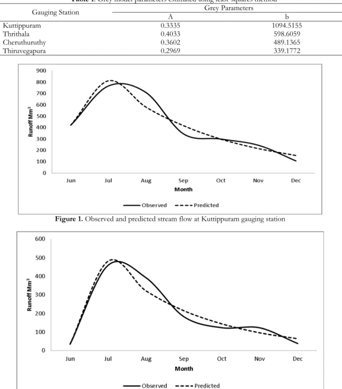
Figure 1. Observed and predicted stream flow at Kuttippuram gauging station
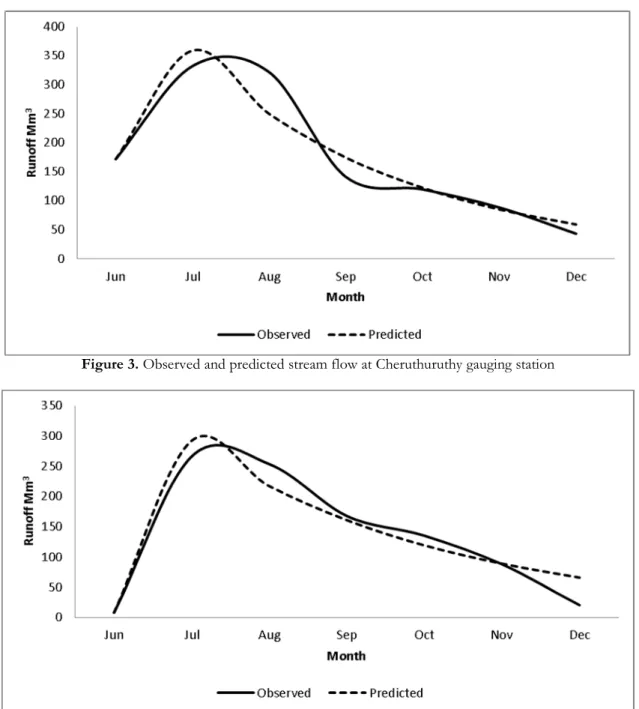
Figure 3. Observed and predicted stream flow at Cheruthuruthy gauging station
Figure 4. Observed and predicted stream flow at Thiruvegapura gauging station
Table 1. Proporsionality constant in temperature change equation
Gauging Station RMSE1 NSE2 CC3 TIC4
Kuttippuram 61.5441 0.9245 0.9619 0.0659
Thrithala 34.7194 0.9502 0.9750 0.0705
Cheruthuruthy 32.0506 0.9043 0.9514 0.0798
Thiruvegapura 25.0713 0.9309 0.9656 0.0766
1. RMSE-root mean square error, 2. NSE-Nash–Sutcliffe model efficiency, 3. CC-correlation coefficient, 4. TIC-Thiel's inequality coefficient
The observed and predicted stream flow hydrographs are shown in Figure 1 to Figure 4. It can be observed from these figures that the actual and estimated values, especially the peak value, are in fairly good agreement. There is a close agreement in the rising limb of the observed and predicted stream flow graphs. Even though the recession segments of the observed and predicted stream flow hydrographs follow the same trend, the fluctuations in the observed values were smoothened out in the predicted curve. The model performance is evaluated by a number of statistical indices such as root mean square error (RMSE), Nash–Sutcliffe model efficiency coefficient (NSE),
18
correlation coefficient (CC) and Thiel’s inequality coefficient (TIC). These indices for the grey prediction models for different gauging stations are given in Table 2. Coefficient of correlation values near to one indicates good correlation. The Nash–Sutcliffe model efficiency values are closer to one, indicating good model accuracy. The Thiel’s inequality coefficient’s values (TIC) are closer to zero, indicating a better forecast method. All the quantitative statistical performance indicators show the suitability of the grey system prediction models to the study area.
Conclusion
Grey system prediction models derived for the study area were able to predict stream flows revealing close agreement with the observed flows as could be seen from their plot. The statistical model performance indicators confirmed the ability of the models to predict stream flows with accuracy in the area under study. The grey system analysis seems to be a boon to areas with scarcity of reliable long duration hydrological records.
Nomenclatures
AGO = accumulated generating operation IAGO = inverse accumulated generating operation
GM(h, N) = hth order derivate Grey Model with N number of variables
= original time series data taken consecutively at equal time interval = sequence of raw data values (i.e. time series data like rainfall) = number of observed time series data
= the future predicted value of
= sequence obtained through accumulating generation = an integer variable such that
= index variable that can take values from 1 to n
= the background value which is taken to be the mean of the entries in = summation index which runs from 1 through
‘t’ = time
‘a’ = grey parameter called “developing coefficient” which is a grey response function in decay of the storage capacity and physiographical factors of the grey process in the watershed.
‘b’ = grey parameter called “the grey input” which is a grey response function explaining factors of watershed characteristics responsible for variation in stream flow other than that of ‘a’.
= first order inverse AGO (1-IAGO)
= time index variable that can take values from 1 to n ; k=0,.., n-1 = predicted values of
; k=0,.., n-1 = predicted values of RMSE = root mean square error
NSE = Nash–Sutcliffe model efficiency CC = correlation coefficient
TIC = Thiel's inequality coefficient Mm3 = million meter cube (106 m3)
References
Deng, J. (1982). Control problem of grey system. System & Control Letter, 1(5): 288-294 Deng, J. (1985). Special issue of grey system approach. Fuzzy Mathematic, 5(2): 1-25 Deng, J. (1989). Introduction to grey system theory. Journal of Grey System, 1(1): 1-24.
Gupta, V.K., and Duckstein, L. (1975). A stochastic analysis of extreme droughts. Water Resources Research, 11(2): 221-228.
Lee, R. H., and Wang, R. Y. (1998). Parameter estimation with colored noise effect for differential hydrological grey model. Journal of Hydrology, 208: 1-15.
Liu, S., and Lin, Y. (2006). Grey Information. Springer Verlag Inc., London.
Trivedi, H.V., and Singh, J.K. (2005). Application of Grey System Theory in the Development of a Runoff Prediction Model. Biosystems Engineering, 92 (4): 521-526.
Viertl, R. (1990). Statistical inference for fuzzy data in environmetrics. Environmetrics, 1(1): 37-42.
Wen, K. L. (2004). The grey system analysis and its application in gas breakdown and VAR compensator finding. Journal of Computational Cognition, 2(1): 21-44.
Xia, J. (1985). Conceptual model of hydrologic nonlinear system and grey parameters identification. Wuhan Institute Hydraulic Electrical Engineering, 2(55).
Xia, J. (1989). Research and application of grey system theory to hydrology. Journal of Grey System, 1(1): 43-52. Xia, J. (1990). A grey system approach applied to catchment hydrology. In: The Hydrological Basis for Water
Resources Management. IAHS Publ. No. 197.
Yu, P. S., Chen, C.J., Chen, S.J., and Lin, S.C. (2001). Application of grey model toward runoff forecasting. Journal of the American Water Resource Association, 37(1): 151-166.