1
CONSISTENT ESTIMATION OF CONDITIONAL CONSERVATISM
Manuel Cano-Rodríguez
Universidad de Jáen - Department of Financial Economics and Accounting
Manuel Núñez-Nickel
Universidad Carlos III de Madrid – Department of Business Administration
November, 2010.
The authors are indebted to Beatriz Moreno, Bing Guo and Juan Manuel García-Lara for their useful comments. This research is funded by the SEJ2007-65782-C02-02ECON and the ECO2010-22105-C03-03 (subprogram ECON) research projects of the Spanish Ministry of Science and Education, and the INFOINNOVA research project of the Community of Madrid.
2
CONSISTENT ESTIMATION OF CONDITIONAL CONSERVATISM
Abstract
In this paper, we propose an econometric model that presents three advantages in relation to the Basu model: (1) it is robust to the aggregation problem; that is, we prove that the Basu model produces inconsistent estimations of conditional conservatism and that this problem is solved with our proposal; (2) it can produce firm-specific measures of conservatism by using time-series; and (3) it completes the understanding of the intercept in the Basu model by breaking it down between unconditional conservatism and the reversion of the differences between market and book values of equity. In other words, we can provide firm-specific measures of both conditional and unconditional conservatism with the same model. We demonstrate all these theoretical assertions using simulated data.
Keywords: accounting conservatism; conditional conservatism; unconditional conservatism; the Basu model; aggregation effect.
1. INTRODUCTION.
In this paper, we demonstrate that the Basu model produces inconsistent estimates of the relation between accounting earnings and good and bad news. To prove it, we develop a theoretical framework, based on realistic and simple assumptions, which describe the relation between the variations in the market value of equity and accounting net income. Then, we analyze the capability of the Basu model for
producing consistent estimates of the relation between accounting net income and the variations of market value of equity for our theoretical framework, demonstrating theoretically that, except under very restrictive conditions, the Basu model is affected by the aggregation effect described by Givoly et al. (2007). More specifically, we show that aggregation bias makes the Basu model overestimate the influence of good news on earnings and underestimate the influence of bad news on earnings.
Additionally, we propose an econometric model, based on Basu’s definition of conservatism, which is robust to the aggregation effect. This model can be estimated using time-series methodology in a wider range of cases than the Basu model, facilitating the obtaining of firm-specific measures of both conditional and
3
unconditional accounting conservatism. Finally, we empirically prove every assertion using simulated data.
The remainder of the paper is structured as follows: first, Section 2 remembers the Basu model and its problems; in Section 3, we develop the theoretical framework to analyze the relation between accounting earnings and the variation of the market value of equity; in Section 4, we demonstrate that the Basu model produces inconsistent estimations of the return-earnings relationship except in very restrictive situations; in Section 5, we develop our econometric proposal; in Section 6, we compare the capability of Basu and our model to produce consistent estimates of the relation
between earnings and returns, applying both models to simulated data; Finally, Section 7 concludes.
2. DESCRIPTION OF THE BASU MODEL AND ITS PROBLEMS.
The Basu model (Basu 1997) relies on the assumption that accounting conservatism leads to a faster recognition of bad news than good news. Consequently, the
contemporaneous relation between negative market returns (as a proxy of bad news) and accounting earnings is expected to be higher than the contemporaneous relationship between positive market returns (as a proxy of good news) and accounting earnings. According to this, the Basu model can be expressed as shown in equation (1)1:
0 1 0 1
t t t t t t
ANI d M d M (1)
Where ANIt is the accounting net income obtained in period t; ΔMt is the variation in the market value of equity during period t; dt is a dummy variable that equals one if ΔMt is negative and zero otherwise; and εt is the error term. Parameter β0 captures the relation between earnings and positive increments in the market value of equity, while
parameter β1 captures the difference in the reaction of earnings to the reductions in market value of equity compared to the increments in the market value of equity. Parameters α0and α1are the intercepts of the model.
Consistently with the hypothesized differential timeliness, Basu obtains that the reaction of earnings to negative market returns is greater than the reaction to positive market returns, thereby producing a positive value for coefficient β1. From this seminal work,
1
Although Basu deflates all the variables of the model by the beginning-of-period market value of equity, we have preferred to present the equation without deflating because previous literature has indicated that the use of this deflator can produce a bias in the estimates of the parameters, produced by the empirical relationships between share prices, return variance and the probability of reporting a loss (Patatoukas and Thomas 2009).
4
the Basu model has become one of the prevalent models for testing the existence of accounting conservatism (Ryan 2006; Ball et al. 2009; Khan and Watts 2009). However, and despite its popularity, previous literature has pointed out that the Basu model presents various weaknesses that put into question the validity of its results (Dietrich et al. 2007; Givoly et al. 2007; Patatoukas and Thomas 2009). In this paper, we focus on two important drawbacks of the Basu model. The first one is the difficulty to obtain firm-specific measures of accounting conservatism. Although, in theory, these firm-specific measures could be obtained using firm-specific time-series estimations, in practice this method is likely to produce noisy estimates of the coefficients because few companies have a sufficient number of years with negative returns for the time-series estimation of the model (Zhang 2008)2.
The second drawback is the aggregation effect: the Basu model does not estimate the influence of each economic individual gain or loss on accounting net income, but the relationship between net income and the aggregation of all the economic gains and losses of the period, because the exogenous variable is the total market return of the period. This problem has been initially detected by Givoly et al. (2007), who, using simulated data, obtain that the coefficient that measures the earnings differential timeliness drops as the number of economic events in a period increase. Besides, this fall in the value of the coefficient is more evident when the positive and negative shocks are identically distributed, making the compensation between the economic gains and losses of the same period more likely. They conclude that the aggregation problem produces a dissipation of the evidence of conservatism when the different economic events of a period are likely to offset each other.
3. A THEORETICAL FRAMEWORK OF THE RELATION BETWEEN
ACCOUNTING EARNINGS AND MARKET RETURN
In this section, we derive a theoretical firm-specific model that relates the variations in the market value of equity and accounting earnings. First, we expose how good and bad news is incorporated into the market value of equity in a timely manner; then, we will describe the formation of accounting earnings and its relation with the variations of the market value.
2
In its extreme, coefficient β1 (β0) could not be estimated for those companies with no negative (positive)
5
3.1. The influence of good and bad news on market return
Under the assumption that capital markets are efficient, we can expect market prices to reflect all the publicly available information in a timely way (Ball, Kothari et al. 2009). Consequently, the market value of equity will be equal to the present value of the expected future cash flows of the firm. Additionally, any change in that present value produced by an unexpected event will be instantaneously incorporated into the market value of equity. Another consequence of market efficiency is, moreover, that price variations will be serially uncorrelated.
The market value of equity at any given moment t can be obtained by the following expression: 1 t t t M M M (2)
Where Mt is a random variable that symbolizes the market value of equity at the end of
period t, and Mt-1 is the market value of equity at the beginning of period t; ΔMt is the sum of all the variations (increases and decreases) in the market value of equity, occurred between t-1 and t. According to this definition, ΔMt can be computed as:
, 1 t
nt j t j M m (3)Where nt is the number of economic events that alter the market value of equity between
t-1 and t, and Δmj,t the variation in the market value produced by each event. We assume Δmj,t to be stationary and symmetric random variables that are serially
uncorrelated. In other words, nt can be interpreted as the number of variations in the
stock price of a firm during a given period (a year, a trimester, a month, a day…), and Δmj,t as the values of each individual variation.
Let us now consider that some of the events of the period are “good news” (that is, they produce an increase in M) and the remainder of the events are “bad news” (produce a
decrease in M). We denote the positive variations in the market value of equity
produced by good news as Δm+j,t. Thus, Δm+j,t will be equal to Δmj,t if Δmj,t is positive,
and zero otherwise. Analogously, Δm-j,t represents the negative variations in the value of M, consequence of the occurrence of bad news. Hence,Δm-j,t will be equal to Δmj,t if
Δmj,t is negative, and zero otherwise. By introducing Δm+j,t and Δm-j,t in equation (3),
6 , , 1 1 t
nt j t
nt j t j j M m m (4)For simplicity, we denote , 1
nt j t j m by ΔM+t and , 1
nt j t j m by ΔM-t. ΔMt would therefore be: Mt Mt Mt (5)Put simply, expression (5) indicates that the total variation in the stock price during a period can be calculated as the sum of the entire positive and all the negative variations produced between the beginning and the end of that period. For example, the net variation in the stock price during a year can be calculated as the sum of all the positive and negative monthly (or weekly, or daily…) variations which have occurred in that year.
3.2. The influence of good and bad news on accounting net income
In this theoretical model, we assume that the accounting net income does not reflect the economic gains and losses with the same timeliness as the market value. The reason is that the accounting gains or losses are not recorded unless they meet the accounting recognition criteria, based on requirements of verifiability, objectivity and conservatism. Some economic gains/losses can meet these accounting requirements in the same period that they are generated, and, consequently, they will affect the market and the book value of equity in that same period (for example, an unexpected increase in sales in the current period that is not expected to affect the sales of the future periods). Some other economic gains or losses, however, can fulfil those requirements only partially. In this case, the market value of equity will be affected by the total amount of the gain/loss, but the accounting net income will incorporate just the portion of that economic gain/loss that meet the recognition criteria. The remainder of that economic gain/loss will be recognized in future periods, as it fulfils the accounting requirements (an example could be an unexpected increase in sales in the current period that is expected to affect also the sales of the future periods. In this case, the present value of all the expected variations in
7
the cash flows will be incorporated into the stock prices, but only the increase in the sales of the current period will be recognized as net income in this period. The rest of the value, created by the expectations of future sale increases, will be recorded in the future, as such increases are realized).
Finally, we can also consider other economic gains/losses that, despite the fact that they can affect the market value in the current period, do not meet the requirements to be included in the accounting income of this period. These economic gains/losses, though, will be recorded as gains/losses in the future, when they meet the required conditions (for example, the potential capital gains in fixed assets that are valued in accounting at their purchase cost will be recognized in the market value of equity, but those potential capital gains will not be recognized in accounting until the asset is sold).
Given that under accounting conservatism losses are timelier than gains (Basu, 1997) we incorporate this possibility by differentiating between economic gains and losses. Accounting net income is hence expressed as follows:
, , , , 1 1
nt
nt t t j t j t j t j t j j ANI m m (6)Where ANIt represents the accounting net income of period t. β+j,t and β-j,t indicate the
portion of the economic gain Δm+j,t or the economic loss Δm-j,t, respectively, that meet
the requirements to be registered as an accounting gain or loss in the period t. We assume that β+j,t and β-j,t are stationary and symmetric random variables with means
and , respectively. We also assume that they are not correlated over time and that they are independent from the amount of the economic gain or loss (Δm+j,t or Δm -j,t).
Finally, αt is the portion of the accounting net income that is independent of the
economic gains or losses of the same period t. We will discuss later the composition of this αt.
According to the former theoretical framework, the value of β+j,t and β-j,t ranges from 0
to 1, both inclusive. Thus, if the effect of the unexpected event meets the accounting requirements to be fully incorporated into the accounting net income of the current period, the value of the beta parameter will be equal to 1, and the variation of the market and the book values of equity produced by the economic event will coincide. When only
8
a portion of the variation of the market value of equity meets the accounting requirements to be recorded in the current year, the beta coefficient indicate the
proportion of the total change in the market value that is recorded, this proportion being between zero and one. In this case, the variation that the economic event has produced in the market value of equity will be higher than the variation produced in the book value of equity. Finally, if the economic effect of the unexpected event does not meet the accounting criteria to be recognized as a gain or a loss in the current period, the value of the parameter beta will be equal to zero. In this case, we obtain that the economic event produces a variation in the stock market of equity but no variation in the book value of equity.
4. AN EVALUATION OF BASU MODEL ESTIMATES
In this section, we evaluate if Basu’s model correctly captures the relation between accounting net income and market returns described in the theoretical framework, demonstrating that, under normal conditions, the estimated parameters are inconsistent estimations of the relationships between accounting net income and positive and negative variations in market value.
In order to facilitate this evaluation, we add and subtract , , 1 t n j t j t j m
in equation (6) obtaining that:
, , , , , , 1 1 1 , , , , , 1 1 t t t t t n n n t t j t j t j t j t j t j t j j j n n t j t j t j t j t j t j j ANI m m m m m
(7)Consequently, according to the theoretical framework, the average contemporaneous relationship between earnings and good news is captured by the expectation of j t, (that is, ); the average contemporaneous relationship between earnings and bad news is the expectation of j t,
( ); and the difference between t and t indicates the existence of a difference in the timely accounting recognition of gains and losses.
9
Next we evaluate if the Basu model rightly captures the contemporaneous relation between market value variations and accounting earnings. For doing so, Basu’s coefficient β0 should be an unbiased estimator of , that is, the contemporaneous relationship between accounting net income and the effect of good news on market value; similarly, the coefficient β1 should be an unbiased estimator of , that is, the difference in the timely recognition of gains and losses. Next, we analyze if the Ordinary Least Squares (OLS) estimations of the Basu model coefficients are unbiased estimators of those parameters of our theoretical model.
4.1. Basu’s estimates of the influence of good news on accounting net income.
In this section, we present the demonstration of our first proposition.
Proposition 1: In presence of accounting conservatism, the Basu model overestimates the influence of good news on accounting earnings, except if, and only if, there is no bad news in the periods with positive market returns.
Let ˆ0denote the Ordinary Least Squares (OLS) estimation of β0 from equation (1). The value of this ˆ0 converges in probability in:
0 , 0 ˆ lim 0 t t t t t Cov ANI M M p Var M M (8)In Appendix A, we demonstrate that, under the assumptions of the former theoretical framework, the value of expression (8) is the following:
0 , 0 ˆ lim 0 t t t t t Cov M M M p Var M M (9)Indicating that ˆ0is a biased estimator of except if one of the two following conditions is met:
10
Condition 1: . In this case, there is no differentiation in the timely recognition of good and bad news. Therefore, there is no accounting conservatism.
Condition 2: Cov
Mt,Mt Mt 0
0. As is demonstrated in the Appendix A, this condition will be met if, and only if, there is no bad news in the periods of positive values of market returns.We consider these conditions too restrictive. On the one hand, conservatism is a common principle in accounting, what implies that it is reasonable to expect that the financial statements of the companies will be conservative, and neither neutral nor aggressive. Consequently, we consider that condition 1 is not a realistic condition, it being more appropriate to expect that .
Condition 2, on the other hand, implies that there will be no bad news in those periods for which the market return is positive. In other words, this condition requires that, if the stock price has risen during a given period (a month, a trimester, a year…), all the variations in the price during that period must be positive. We also consider this situation unlikely, the existence of both good and bad news in the same period being more likely. In this case, as it is demonstrated in Appendix A, the value of
t , t t 0
Cov M M M is positive.
Consequently, if none of the two former conditions are met, the value of the parameter 0
ˆ
will be a biased estimator of , with the bias being higher than zero. That is to say, in normal conditions, the Basu model overestimates the reaction of accounting net income to good news
ˆ0
.4.2. Basu’s estimates of the differential influence of bad news on accounting net income.
Our second proposition is the following:
Proposition 2: In presence of accounting conservatism, the Basu model underestimates the influence of bad news on accounting earnings, except if, and only if, there is no bad news in the periods with positive market returns and no good news in the periods with negative market returns.
11
Let now ˆ1 represent the Ordinary Least Squares (OLS) estimation of the parameter β1 from equation(1). The value of ˆ1 converges in probability in:
1 , 0 , 0 ˆ lim 0 0 t t t t t t t t t tCov ANI M R Cov ANI M M
p
Var M M Var M M
(10)
Under the assumptions of the theoretical framework, the former expression is equal to (see Appendix B for demonstration):
1 , 0 , 0 ˆ lim 0 0 it t t it t t t t t t Cov m M M Cov m M M p Var M M Var M M
(11)Consequently, ˆ1 will be an unbiased estimator of
, only if at least one of the following two conditions is met:Condition 1:
=0, that is to say, if there is no differentiation in the timely recognition of good and bad news and, therefore, no accounting conservatism.Condition 2: If the expression in brackets in equation (11) is equal to one. However, as demonstrated in Appendix B, this will happen only if the two following conditions are met:
Condition 2.1: if in a given period the stock price rise, all the changes in the stock price of that period must be positive.
Condition 2.2: if in a given period the stock price fall, all the changes in the stock price of that period must be negative.
Again, we consider unlikely the inexistence of bad (good) news in the periods of positive (negative) market returns. In the case that both good and bad news occur in the same period, as is demonstrated in Appendix B, the value of
, 0 , 0 0 0 it t t it t t t t t t Cov m M M Cov m M M Var M M Var M M
is lower than one, underestimating the difference in the timely recognition of gains and losses.
12
As we have demonstrated in section 4, except under very restrictive conditions, the Basu model produces biased estimations of the relation between market returns and accounting net income because of the aggregation effect. In this section, we propose an alternative empirical model that presents the following advantages over the Basu model: (1) it overcomes the aggregation effect suffered by the Basu model; (2) it can be applied to a wider set of firms in a time-series setting to estimate firm-specific measures of conservatism; and (3), we also analyze the formation of the constant of the model to obtain a firm-specific measure of unconditional conservatism.
We start our model from equation (6). Since j
and j
are assumed symmetric random variables, we can express them as follows:
j j j j (12)
Where j and j are the deviations from the expectation of j and j, respectively. The mean of these two variables is zero and they are independent from the other random variables, particularly from mjand mj. Substituting (12) in (6), we obtain:
, , , , 1 1 , , , , 1 1 , , , , , , 1 1 1 t t t t t t t n n t t j t j t j t j t j j n n t j t j t j t j t j j n n n t j t j t j t j t j t j t j j j ANI m m m m m m m m
(13) Finally, if we define , , , , 1 t n t j t j t j t j t j m m
, we obtain: t t t t t ANI MM (14)That is the first version of our empirical model. Since ξt is a random variable with null
mean and independent of Mt and Mt, the OLS estimation of expression (14) will produce consistent estimates of and .
We focus now on the intercept of equation (14). As it has been indicated above, this parameter captures the accounting gains and losses registered on period t that do not proceed from the variations of the market value of equity occurred in the same period. These gains and losses can, then, proceed from three different sources:
13
a) First, they can be gains and losses that affected the market value of equity in previous periods, but have not met the requirements to be recognized as accounting gains or losses until the current period. Therefore, these gains and losses are already incorporated into the market value of equity at the beginning of the period (Mt-1), but not into the book value of equity at the beginning of the
period (Bt-1). Consequently, the accounting recognition of these gains and losses
contributes to reduce the difference between the market and the book values of equity.
b) Second, they can be accounting gains and losses that are unrelated to all the current and past market value variations. These gains and losses would be, then, the accounting recognition of potential future economic gains or losses that have not been incorporated into stock prices. However, under the hypothesis of market efficiency, the stock prices will incorporate all the expected future gains and losses. Consequently, these accounting gains or losses would be
overstatements of the potential future gains and losses. Under accounting conservatism, this overstatement is not possible for gains3, but it is possible for losses. This accounting overstatement of potential losses has been named in previous literature as unconditional conservatism. Some examples of these practices would be the overestimation of accounting depreciation, of bad debts or the use of the LIFO method for stock valuation (Qiang 2007). Unconditional conservatism, then, will imply a reduction of the book value of equity (Bt) with
no variation in the market value of equity (Mt).
c) Finally, unconditional conservatism practices produce a downward bias in book value of equity compared to market value of equity, but this bias will tend to disappear over time, when the overstated losses are realized. For example, an overstated depreciation of a fixed asset will produce an understatement of book value of equity compared to market book of equity, but this understatement will disappear when the fixed asset is sold and the capital gains are recognized in the accounting net income. The consequence of this reversion of unconditional conservatism will be a reduction of the difference between the market and book values of equity.
14
In summary, the intercept of the model for a given period t is formed by two
components: (1) the amount of unconditional conservatism recorded in period t; and (2) the reversion of unconditional conservatism recorded in previous periods and the recognition of market value variations that are recognized as gains or losses in the period t. Since both the reversion of unconditional conservatism and the recognition of market value variations of previous periods contribute to reducing the difference between market and book values of equity, αt can be computed as:
1 1
t UCt t Mt Bt
(15)
Where δt indicates the portion of the difference between Mt-1 and Bt-1 that is
incorporated into ANIt as a consequence of the recognition of past variations of market
value and/or the reversion of past unconditional conservatism; and UCt is the overstatement of losses recorded between t-1 and t.
Substituting the value of αt in equation (14), we obtain:
1 1
t t t t t t t t
ANI UC M B MM (16)
Transforming expression (16) into an empirical model, we obtain the final version of the alternative model:
1 1 1 2 3
t t t t t t
ANI a b M B b M b M (17)
Where a is the intercept of the model and captures the level of unconditional
conservatism of the company (UCt); coefficient b1 captures the portion of the difference
between the market value and the book value of equity at the beginning of the period, a consequence of past unregistered gains and losses as well as unconditional conservatism in previous periods, that is recognized in accounting in the current year (δt); and
coefficients b2 and b3 represent, respectively, the proportion of market gains and losses produced between t-1 and t that are recognized as accounting net income in the current period ( and , respectively).
6. AN EMPIRICAL COMPARISON OF BASU MODEL AND THE
ALTERNATIVE MODEL.
In this section, we use simulated data to analyze the performance of the original Basu model in comparison to the alternative model. The reason for using simulated data is that, by doing so, we can compare the results of both models with the true values of the variables used in the simulation process.
15
6.1. Description of simulated data.
To test the former models, we iterate the following process. In each iteration we
produce the simulations of the data of a single firm during 400 periods, composed of 75 market sessions each. Each period is intended to represent a quarter of the economic year, comprised of 75 stock market sessions each. We denote each period by the sub-index t and each session of the period t by the sub-index j. For simplicity, we consider that in each session we obtain a single economic event. That event can be a good news event (and, therefore, increases the market value of equity) or a bad news event (and, therefore, decreases the market value of equity).
We set the initial values of market value (M0) and book value (B0) of equity to 100. Then, we proceed as follows for each session j of each period t:
a) We generate a random number from a uniform distribution between 0 and 1 to determine the sign of the event. We denote this number by pj,t. If pj,t exceeds 0.5, a good news event occurs. Otherwise, a bad news event occurs.
b) If a good news event occurs (pj,t>0.5), we generate the impact of that event on the market value of equity from a normal distribution, with mean +1 and standard deviation 0.2. We denote this impact by mj,t+.
c) If a bad news event occurs (pj,t<0.5), the impact of that event on the market value of equity is generated from a normal distribution, with mean -1 and standard deviation 0.2. We denote it by mj,t-.
d) We define the variation in the market value of equity occurred on session j of period t (mj,t) as mj,t++ mj,t-.
e) If a good news event occurs a (pj,t>0.5), a βj,t+ parameter is generated from a
normal distribution with mean 0.3 and standard deviation 0.05. This parameter indicates the portion of the positive market variation mj,t+ that is recorded on the
accounting net income of period t.
f) If a bad news event occurs (pj,t<0.5), we generate a βj,t- parameter from a normal
distribution with mean 0.7 and standard deviation 0.05. This parameter indicates the portion of the negative market variation mj,t- that is recorded on the
accounting net income of period t.
g) We define the recognition of the market variation of session j of period t in the accounting net income as j t,mj t,j t,mj t,
16
Then, we compute the following data for each period:
i) The total market value variation of each period t is calculated as the sum of the market variations of all the sessions of that period:
75 , 1 t j t j M m
. We also generate a dummy variable dt that is equal to 1 if ΔMt is negative, and zero otherwise.ii) We compute the accumulated positive market variation of the period as the sum of the positive market variations of the period:
75 , 1 t j t j M m
iii)We calculate the accumulated negative market variation of the period as the sum of the negative market variations of the period:
75 , 1 t j t j M m
iv) The market value of equity at the end of the period t is calculated as 1
t t t
M M M
v) We generate a parameter δt from a normal distribution of mean 0.5 and standard deviation 0.05 to indicate the portion of the difference between the market and the book values of equity at the beginning of the period t that is incorporated into the accounting net income of t. We also generate a random value from a normal distribution of mean -5 and standard deviation 1to simulate the
accounting overstatement of losses (unconditional conservatism). We denote this number by UCt.
vi) We then compute the accounting net income of the period
as
75 1 1 , , , , 1 t t t t t j t j t j t j t j ANI UC M B m m
vii)The book value of equity of period t is computed as Bt Bt1ANIt
After generating the former data, we estimate the Ordinary Least Squares estimations of the following firm-specific regression models:
Model 1. the original Basu model:
0 1 0 1 1
t t t t t
ANI d M d M (18)
Model 2. Alternative model:
0 1 1 1 0 1 2
t t t t t
ANI a a M B b M b M (19)
17
Then, we compute the means of the estimations of the parameters of equations (18) and (19) obtained from the 5.000 iterations, in order to test if they are statistically different from their theoretical values.
Thus, regarding Basu’s original model, parameter β0 is intended to capture the relation
between the positive variations in market value and the accounting net income. In our simulated data, this relation is normally distributed, with a mean of 0.3. Therefore, β0 must not be significantly different from 0.3 to be an unbiased estimator of the relation between positive variations in market value and accounting net income. On the other hand, parameter β1 tries to capture the difference between the influence of the negative market variations and the influence of the positive market variations on accounting net income. In our simulated data, the relation between negative market variations and accounting income is normally distributed with a mean of 0.7. Consequently, the difference between the relation of negative and positive market variations is normally distributed with a mean of 0.4 (0.7–0.3). Parameter β1, hence, must not be significantly different from 0.4 to be an unbiased estimator of the incremental influence of bad news, compared to good news, on accounting earnings.
Parameters b0 and b1 of the alternative model measure the portion of stock price rises or reductions, respectively, which occurred during the period t and have not been recorded in the accounting net income of the same period. In our simulated data, the expected relation between positive market variations and net income is normally distributed with mean 0.3, while the expected relation between negative market variations and net income is also normally distributed with mean 0.7. Parameters b0 and b1, then, must not
be significantly different from 0.3 and 0.7.
6.2.Simulation results.
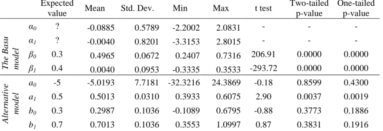
Table 1 reports the descriptive statistics of the estimations of models (18) and (19). Parameter β0 obtains a mean value of 0.4965, which is significantly higher than the expected value of 0.3. This result confirms that the Basu model, owing to the
aggregation problem, overstates the relation between positive returns and accounting net income. On the other hand, the mean value of parameter β1 is 0.0040. This value, albeit positive, is significantly lower than its real value (0.4), confirming that the aggregation problem leads the Basu model to underestimate this parameter.
18
The results for the alternative model parameters are totally different. The mean value of
b0 is 0.2987, and the value of the t test (-0.88) does not reject the null hypothesis of this mean being equal to the real value of the parameter (0.3); regarding b1, its value is
0.7013 with a t – value of 0.87, that does not reject the null hypothesis of this mean being equal to 0.7.
These results confirm that the alternative model is robust against the aggregation effect observed for the original Basu model, because it captures the relation between market returns and accounting net income without bias.
Additionally, the alternative model presents a second advantage over the original model: its better applicability in time-series fashion. As we have pointed before, the time-series estimation of the Basu model is not feasible for those companies without years of negative market returns (or without years with positive market returns), and it is likely to produce noisy estimates of the coefficients when the number of years with negative returns is too low. The alternative model, however, does not require a minimum number of years with negative returns, but simply the existence of some sessions with negative market returns. This weaker requirement makes the alternative model more suitable to obtain firm-specific measures of conservatism using time-series estimation.
A third advantage of the alternative model is that it analyzes the composition of the intercept, differentiating between unconditional conservatism and the reversion of the differences between book and market values of equity.
Regarding the mean of the estimates of unconditional conservatism (parameter a0), it
does not differ significantly from the expected value (t – value of -0.18), showing that the alternative model also estimates this parameter without bias.
Finally, the mean of the estimates for the parameter of the reversion of the differences between book and market values (parameter a1) is slightly higher than the expected
value. This bias in the estimation of the parameter a1 can be produced by the
auto-regressive nature of the alternative model4, since the OLS estimates of auto-regressive models are consistent but unbiased, what implies that those estimates are biased in small samples (Tanizaki 2000)5. Although there are various methods that can be employed for correcting this bias (see, for example, Kim 2003), we consider it preferable to use the
4
In the modified model, ANIt is a function of Mt-1 – Bt-1 that, in turn, can be expressed as Mt-2 – Bt-2 + Mt-1
– ANIt-1. Consquently, ANIt is dependent on ANIt-1 and the model presents an auto-regressive structure.
5 The bias disappears when we make the simulation process using a higher number of periods
(specifically 4,000 quarters instead of 400), supporting that the bias is produced by the small number of periods.
19
traditional OLS method to compare results with previous tests in the same research stream.
6.3. Robustness checks.
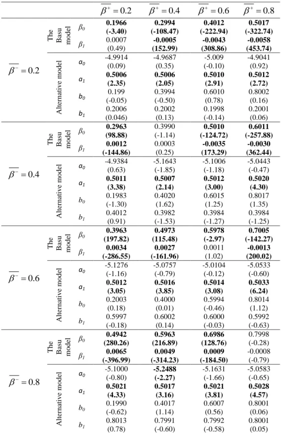
To test the robustness of the alternative model, we have repeated the simulation using different values for the variables that intervene in that process. In Table 2, we present the means of the estimations of the coefficients of the Basu model and the alternative model for different values of the parameters βj,t+ and βj,t-. The other variables of the simulation remained at their initial values.
The results are not qualitatively different from those obtained for the original values of the simulation: the Basu model overstates the relation between accounting net income and good news and understates the relation between accounting net income and bad news, while the alternative model estimates are better estimates of the relation between accounting and both good and bad news. Regarding the portion of accounting net income unrelated to contemporaneous market value variation, the estimates of coefficient a0 are not significantly different from their expected value, obtaining unbiased estimations of unconditional conservatism. However, the estimates of
coefficient a1 are usually higher than the expected value, owing to the bias produce by the size of the sample.
The results reported in this table also support some of our findings about the Basu model estimates. Thus, we have demonstrated that the bias in the estimation of β0 and β1
disappears if the expectation of βj,t+ equals the expectation of βj,t-, , that is to say, when
good and bad news are recognized on the same timely basis. This fact can be observed in Table 2 when 6. Moreover, we also stated that the size of the bias in the estimation of β0 depends on the difference between the expectations of βj,t- and βj,t+. This fact can also be observed in Table 2: the higher the difference between and
, the higher the values of the t – test.
6 Although the means of the obtained values for the parameter β
1 are not significantly different from its
real value (zero) for all the cases, we have obtained that the means of the obtained values for the parameter β0 are significantly different from its real value in two cases (0.2 and 0.6). This bias, however,
disappears when we increase the number of periods (results are not tabulated but they are available upon request), so we consider that it is produced by the bias produced by the auto-regressive structure of the model.
20
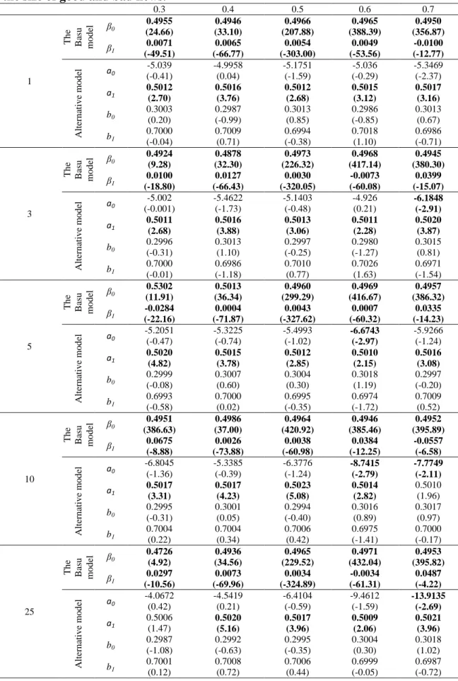
In Table 3, we report the results of the simulation process for various values of the probability of good and bad news and the size of the daily market variations. The results show that the performances of the two models are robust to the changes in these
variables: the Basu model overstates β0 and understates β1, while the alternative model
produces unbiased estimations of parameters b0 and b1. Regarding the parameters a1 and a0, the results for the first are mostly biased, owing to the sample size. The estimates for
parameter a0 are usually unbiased, but we obtain some biased estimations. This bias is
likely to be produced by the sample size too, because it disappears when we increase the number of periods.
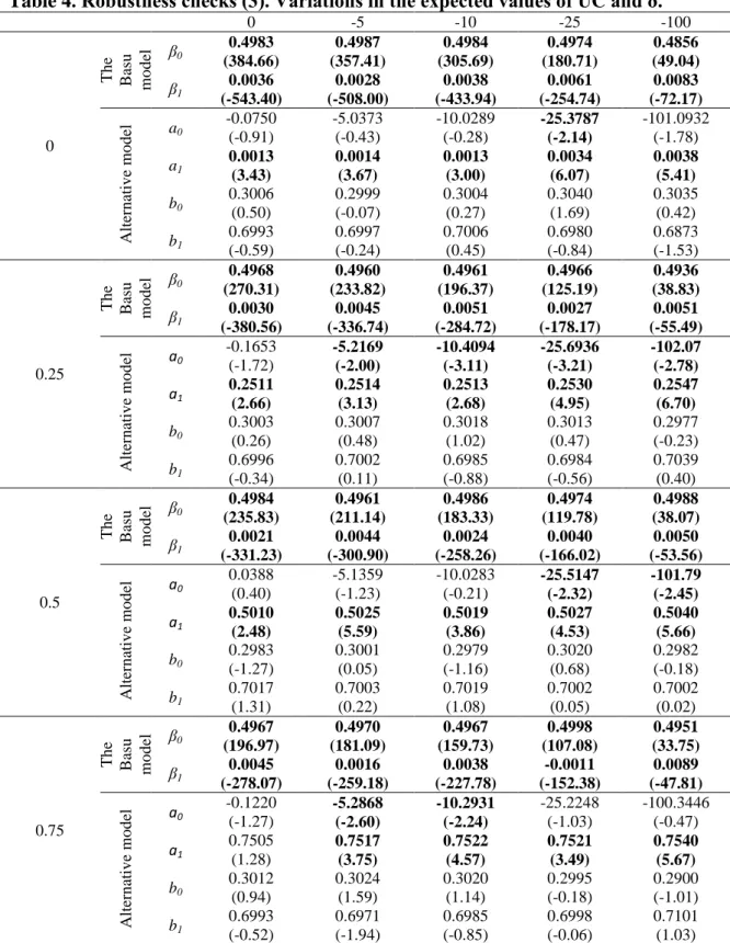
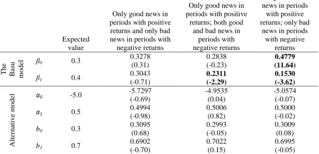
Table 4 presents the results of the simulations for changes in the values of
unconditional conservatism and the δ parameter. The results are qualitatively identical to those obtained in the former tables.
Finally, we also state that the Basu model only produces unbiased estimations of the relation between market value variation and accounting net income in presence of accounting conservatism under very restrictive conditions:
1. For β0, only if the periods with positive market value variation are composed exclusively of positive daily market variations (that is to say, there is no negative daily market value variation in those periods with total positive variations in market value).
2. For β1, only if the periods with positive variations in market value are composed exclusively of positive daily market variations, and the periods with negative variations in market value are composed exclusively of negative daily market variations (that is to say, no negative daily market value variation in the periods with increases in market value of equity and no positive daily market value variation in the periods with decreases in market value of equity).
We empirically test these conditions by studying the estimates of the Basu and alternative models in three particular situations:
In the first situation, the periods with positive (negative) variations in market value are composed only of positive (negative) daily market value variations. To obtain this case, we simulate a uniform random variable between 0 and 1 per period; if the value of this variable is equal to or higher than 0.5, all the daily market variations of the period are simulated from a normal distribution with mean 1 and standard deviation 0.2; if the
21
value of the variable is lower than 0.5, all the daily market variations of the period are simulated from a normal distribution with mean -1 and standard deviation 0.2. In the second situation, the periods with positive market returns are composed exclusively of positive daily market value variations, but the periods with negative market returns are composed of positive and negative daily variations. To obtain this case, we simulate a uniform random variable between 0 and 1 per period; if the value of this variable is equal to or higher than 0.5, all the daily market variations of the period are simulated from a normal distribution with mean 1 and standard deviation 0.2; if the value of the variable is lower than 0.5, we simulate a second uniform random variable between 0 and 1 to simulate the probability of obtaining a negative or a positive market variation in each session of that period. If this second variable is equal to or higher than 0.75, the daily market variation is simulated from a normal distribution with mean -1 and standard deviation 0.2; otherwise, the daily market variation is simulated from a normal distribution with mean 1 and standard deviation 0.2. As can be observed, the probability of bad news is higher (0.75) to ensure that the total market variation of the period is negative.
In the third situation, the periods with positive market returns are composed of both positive and negative daily variations, but the periods with negative market returns are composed only of negative daily variations. The procedure is similar to that described in the second situation, but interchanging the values for good and bad news.
The results of the Basu and the alternative models for these three situations are reported in Table 5. As stated in the theoretical demonstration, when good and bad news are not mixed in the same period (first column of Table 5), Basu’s estimates are not
significantly different from their expected values. Besides, the Basu model also estimate the parameter β0 without bias in the second situation (second column of Table 5), that is to say, when the periods with positive market returns are composed only of positive daily returns. However, the estimate of β1 is significantly biased, because good and bad news are mixed in the periods with negative market returns. Finally, both β0 and β1 estimates are biased when the periods with positive market returns are composed of positive and negative daily market value variations.
In summary, the results of all these robustness tests confirm the conclusions of the theoretical analysis of the properties of the Basu model: in the presence of accounting
22
conservatism, the Basu model produces biased estimations, except when positive and negative daily market value variations are not mixed in the same accounting period.
7. CONCLUSIONS.
Since Basu (Basu 1997) proposed that accounting conservatism can be captured through the contemporaneous relationship between accounting net income and market returns, this has become the most widely employed method to measure accounting
conservatism. However, the Basu model presents two important drawbacks: (1) it is difficult to obtain firm-specific measures of accounting conservatism because in
practice there are few companies with a sufficient number of years with negative returns for the time-series estimation of the model; and (2) it produces inconsistent estimations of the relations between accounting net income and market returns (except under very restrictive situations) because of the aggregation effect.
In this paper we present an intuitive theoretical framework that relates market value variations with accounting net income, and study the performance of the Basu model under the conditions of our framework. We demonstrate theoretically that the Basu model overstates the relation between earnings and positive market returns and
understates the relation between earnings and negative market returns, except if one of the two following conditions is accomplished: (1) absence of accounting conservatism; and (2) all the daily variations of the market value of a given period are of the same sign (that is to say, only positive or only negative daily market variations in a given period). Since these conditions are very unlikely in practice, we conclude that the Basu model is very likely to lead to biased conclusions about accounting conservatism. Consequently, the results of previous papers that have relied on this model should be considered with caution, particularly those that have not found evidence of conditional conservatism, because, as we have demonstrated, the Basu model underestimates conditional conservatism.
In this paper we propose an alternative model that overcomes the former two problems of the Basu model. First, it is easier to implement in a time-series fashion, because it does not require that the firms present both positive and negative market returns for the time series, but simply that the firms present positive and negative intra-period market returns. And, second, it is robust to the aggregation effect and produces unbiased
23
estimations of the relationship between accounting net income and both positive and negative market returns, as we demonstrate with simulated data.
Additionally, we complement our model with an analysis of the portion of the net income that is unrelated to the contemporaneous market returns, dividing it into two components: the first component is the accounting overstatement of losses, also known as unconditional conservatism, and the second component is the reversion of the differences between the market and the book values of equity which occurred in the period. Therefore, the proposed model can produce firm-specific measures of both unconditional and conditional accounting conservatism.
The advantages of the model proposed in this paper are clear both theoretically and for simulated data. However, the next step is to test if the alternative model performs adequately with actual data. In this sense, a potential problem of the model is its auto-regressive structure. Given that actual time-series of data can be much shorter than those we have employed in our simulations, the OLS estimation of the model can suffer from much larger biases produced by the size of the sample, and the application of alternative methods to correct this bias may be necessary.
Finally, despite the fact that the proposed model solves two important problems of the Basu model, some authors have pointed to other weaknesses of the Basu model that are shared by the alternative model, such as the simultaneity problem of the relationship between earnings and stock returns (Dietrich, Muller et al. 2007), the reliance on market efficiency, or the effect of the nature of the economic events on the estimates of the model (Givoly, Hayn et al. 2007). Therefore, although the proposed model is preferable to the Basu model, its results must be considered in relation to the former limitations.
24
Appendix A. βˆ0is a biased estimator of
In this appendix, we demonstrate that ˆ0 is a biased estimator of , except if very restrictive conditions are met.
The probability limit of ˆ0can be obtained as:
0 , 0 ˆ lim 0 t t t t t Cov ANI M M p Var M M (20)We start by calculating the value of the numerator, that is, the covariance between accounting net income and market returns, on the condition that the market return is not negative. To obtain the value of this covariance, we substitute ANIt for its value
according to equation (6):
, , , , , , , , , , , 0 , 0 , 0 , 0 , 0 t t t t j t j t j t j t j t t t j j t t t j t j t t t j a b j t j t j t t t j cCov ANI M M Cov m m M M
Cov M M Cov m M M Cov m M M
(21)Expression a is the covariance between αt and the variation of market value in period t.
Given that αtis the part of the accounting net income that is unrelated to the economic gains and losses of the same period, this covariance is equal to zero.
Next, we calculate the value of expression b. Because it is the covariance of a sum of random variables with another random variable, we express it as the sum of the
covariances between the addends. Further, by applying the definition of covariance, we can rewrite the expression as:
, , , , , , , , , 0 , 0 0 0 0 j t j t t t j t j t t t j j j t j t t t j t j t t t t j Cov m M M Cov m M M E m M M E m M E M M
(22)Where E(.) represents the expectation operator. Given that β+j,t is independent from Δmj,t
for all j,t (and, therefore, it is also independent of ΔMt), and the expectation of β+j,t is
25
j t, t
j t,
t
t 0 j E m M E m E M M
(23)Taking out as a common factor, we obtain:
, , , , 0 0 0 , 0 , 0 , 0 0 j t t t j t t t t j j t t t j t t t j j t t t t t E m M M E m M E M M Cov m M M Cov m M M Cov M M M Var M M
(24)Next, we calculate the value of expression c in equation (21). Following the same steps used to estimate the expression b, we can obtain that the value of c can be rewritten as:
j t, j t,
j t,, t t 0
j t,, t t 0j j
Cov m M M Cov m M M
(25)Substituting the obtained values of a, b and c in equation (20), we obtain that
ˆ0converges in probability to:
, 0 , 0 0 , 0 ˆ lim 0 , 0 0 c b a t t j t t t j t t j t t t j t t bias Var M M Cov m M M p Var M M Cov m M M Var M M
(26)Consequently, the OLS estimation of the parameter ˆ0 will be a biased estimation of the real average influence of good news on earnings, unless the second addend of expression (26) is equal to zero. For this bias to be equal to zero, at least one of the two following conditions should be met:
Condition 1: . In this case, there will be no differentiation in the recognition of good and bad news and, consequently, there would be no evidence of accounting conservatism.
Condition 2: j t,, t t 0 0
j
Cov m M M
. Next, we study the required conditions26
If we substitute ΔMt for its value according to equation (4), we can rewrite the
covariance as: ,, 0 0 ,, , , 0 0 j t t t j t j t j t t j j j j Cov m M M Cov m m m M
(27)Separating the covariance into the sum of two covariances, we obtain:
, , , , , , , , 0 , 0 0 0 , 0 0 j t j t t j t j t t j j j j j t t j t j t t j j j Cov m m M Cov m m M Var m M Cov m m M
(28)The value of the last covariance in expression (28) can be calculated as:
, , , , , , , 0 , 0 , 0 j t j t t i j i t j t t i t j t t i j i j Cov m m M Cov m m M Cov m m M
(29)Given that Δmj,t is serially uncorrelated, Cov
mi t,, mj t, Mt 0
will be null for every i≠j. Therefore, the value of the covariance is:
, , , , , , , , , 0 , 0 0 0 0 i t j t t j t j t t i j j j t j t t j t t j t t j Cov m m M Cov m m M E m m M E m M E m M
(30)According to their definitions, mj t, is equal to zero when mj t, is different from zero, and mj t, is equal to zero if mj t, is different from zero. Therefore, the product of
, j t
m
and mj t, is equal to zero for any value of j. The expectation of this product is, hence, also equal to zero and the value of the covariance remains as follows:
,, , 0 , 0 , 0 i t j t t j t t j t t i j j Cov m m M E m M E m M
(31)Substituting (31) in (28), we obtain that:
, , , , , 0 0 0 0 0 0 j t t t j j t t j t t j t t j j Cov m M M Var m M E m M E m M
(32)27
We can deduce that equation (32) will be verified if, and only if, the two addends are equal to zero, because these two addends are non-negative numbers: On the one hand, the first addend is a variance and, thereby, a non-negative number by definition. On the other hand, the second addend is also a non-negative number, because:
a) The expectation of mj t, is equal or lower than zero for every j, since, by definition, mj t,
takes values that are equal to or lower than zero
b) The expectation of mj t, is positive or zero for every j because, by definition, it takes values that are equal to or higher than zero.
c) Therefore, E
mj t, Mt 0
E mj t, Mt 0
0 d) And, finally,
j t, t 0
j t, t 0
0 j E m M E m M
Consequently, since the covariance is equal to the sum of two non-negative numbers, it will be equal to zero if, and only if, the two non-negative numbers are equal to zero:
, , , , 0 0 , 0 0 0 0 0 j t t j j t t t j j t t j t t j Var m M Cov m M M E m M E m M
(33)Focusing on the condition of the variance equal to zero, we can deduce that:
, 0 0 , 0 0 j t t j t t j Var m M Var m M j
(34)Because mj t, is serially uncorrelated. The conclusion is that the variance of mj t, is null, that is to say, mj t, must be constant for every j. Besides, since mj t, is assumed to be stationary, mj t, will also be stationary, implying that:
, 0 , 0 ,
j t t i t t
m M m M i j
(35)
Finally, for ΔMt being higher or equal to zero, at least one value of mj t, must be non-negative, implying that, for that value of j, mj t, will be equal to zero. We can conclude then that mj t, must be equal to zero for every j:
28 , 0 , 0 , j t t i t t m M m M i j j , , 0 0 j t t j t t m M j m M (36)
In conclusion, the expression j t,, t t 0 0
j
Cov m M M
will be verified, andtherefore, Basu’s parameter ˆ0 will be an unbiased estimator of the relation between good news and accounting income, only if there is no bad news in the periods with positive returns.
If there is at least one bad news in that period, we will obtain that
, 0
j t t j
Var m M
is not equal to zero and, hence, j j t,, t t 0Cov m M M
will be higher than zero. The consequence will be that, in presence of accounting
conservatism (and, thereby, ), Basu’s model will overstate the relation between good news and accounting net income, because ˆ0 will be higher than .
29
Appendix B. ˆ1is a biased estimator of
The following expressi