Optimization Methods for Structured Machine Learning Problems

(1)

Optimization Methods for Structured

Machine Learning Problems

Nikolaos Tsipinakis

A dissertation submitted in partial fulfillment of the requirements for the degree of

Doctor of Philosophy of

University College London.

Department of Statistical Science University College London

(2)

(3)

I, Nikolaos Tsipinakis, confirm that the work presented in this thesis is my own. Where information has been derived from other sources, I confirm that this has been indicated in the work.

(4)

(5)

Abstract

Solving large-scale optimization problems lies at the core of modern machine learn-ing applications. Unfortunately, obtainlearn-ing a sufficiently accurate solution quickly is a difficult task. However, the problems we consider in many machine learning applications exhibit a particular structure. In this thesis we study optimization meth-ods and improve their convergence behavior by taking advantage of such structures. In particular, this thesis constitutes of two parts:

In the first part of the thesis, we consider the Temporal Difference learning (TD) problem in off-line Reinforcement Learning (RL). In off-line RL, it is typically the case that the number of samples is small compared to the number of features. There-fore, recent advances have focused on efficient algorithms to incorporate feature selection via`1-regularization which effectively avoids over-fitting. Unfortunately, the TD optimization problem reduces to a fixed-point problem where convexity of the objective function cannot be assumed. Further, it remains unclear whether existing algorithms have the ability to offer good approximations for the task of policy evaluation and improvement (either they are non-convergent or do not solve the fixed-point problem). In this part of the thesis, we attempt to solve the `1 -regularized fixed-point problem with the help of Alternating Direction Method of Multipliers (ADMM) and we argue that the proposed method is well suited to the structure of the aforementioned fixed-point problem.

In the second part of the thesis, we study multilevel methods for large-scale opti-mization and extend their theoretical analysis to self-concordant functions. In

(6)

par-ticular, we address the following issues that arise in the analysis of second-order optimization methods based either on sampling, randomization or sketching: (a)the analysis of the iterates is not scale-invariantand (b)lack of global fast convergence rates without restrictive assumptions. We argue that, with the analysis undertaken in this part of the thesis, the analysis of randomized second-order methods can be considered on-par with the analysis of the classical Newton method. Further, we demonstrate how our proposed method can exploit typical spectral structures of the Hessian that arise in machine learning applications to further improve the conver-gence rates.

(7)

Impact Statement

In the third chapter we aim to solve the Temporal Difference (TD) learning problem in off-line Reinforcement Learning (RL) which typically is a difficult task and for this reason it cannot find many practical applications specifically when sparsity is required. Our proposed method is tested in a complex environment and our prelim-inary numerical results show an encouraging performance of our method (ADMM-TD). However, a proof of convergence of ADMM-TD is still open. We believe that our encouraging numerical results will drive other researchers within academia to establish a complete theory of ADMM-TD. On the other hand, outside academia, on-line TD learning is already widely used in practice and in many machine learn-ing applications is produclearn-ing sufficiently accurate approximations. With the work undertaken in this chapter we believe that off-line TD learning can be efficiently compared to other techniques applied in machine learning problems. In the fourth chapter of this thesis we study the multilevel methods and we propose YAWN, a variant of the Newton method. In large-scale optimization, randomized variants of the Newton method have concentrated the main interest of the research commu-nity due to their fast convergence rates. However, their analysis suffers from one the following shortfalls: (a) is not scale invariant, (b) is not global, (c) absence of super-linear convergence rates —we note that all three characteristics are involved in the analysis of the classical Newton method. In this part of the thesis, we claim that our proposed method is able to address all three issues. Hence, with the analy-sis undertaken in this chapter, the analyanaly-sis of the randomized variants of the Newton method can be considered on par with the classical analysis of the Newton method.

(8)

The super-linear convergence of YAWN can be further improved by estimating spe-cific parameters of the algorithm, something that can attract the interest of other researchers within academia. On the other hand, outside academia, we argue that YAWN can be directly applied in practice and be able to produce accurate results quickly. This is also demonstrated in our initial numerical experiments which sug-gest that YAWN outperforms state-of-the-art methods.

(9)

pass through solitude and difficulty, isolation and silence in order to reach forth to the enchanted place where we can dance our clumsy dance and sing our sorrowful song”

(10)

(11)

Acknowledgements

My Ph.D. journey started almost four years ago. For me being today at the position of submitting my thesis is very much ought to my first supervisor Dr. James D.B. Nelson. When I was applying for the Ph.D position in University College London I was not believing that I would be accepted in such a prestigious institution. It was James then that trusted me and offered me this position. I would like to express my deepest gratitude to my supervisor James Nelson. Unfortunately, sad things happen in life. James is not with us anymore. I would like to express my deepest condolences to his family and once more to mention that I am extremely grateful to him.

After James loss the situation was difficult for me and the rest of his Ph.D students. We had to seek new supervisors. By this time, I had already been in discussions with Dr. Panos Parpas, Imperial College London, in order for us to begin a collab-oration since we are both interested in computational optimization. I asked Panos to supervise me for the rest of my Ph.D. and I after explained him the situation he immediately accepted to co-supervise me. He, of course, had no obligation to ac-cept and unofficially supervise a student from another university. I would like to express that I am extremely thankful to Panos for this decision. Since I was a rookie in optimization, Panos was the best teacher I could have. His amazing research experience in optimization methods brought me today in the position of submitting my thesis. I shall mention that the great job that appears in Chapter 4 of this thesis is ought to him. I could never be able to produce such good results if I did not have

(12)

his guidance. Panos is a great person and supervisor and I would clearly like to continue collaborating with him in the future either officially or unofficially. During my Ph.D. studies, I have to admit to myself that I feel extremely lucky to meet great people and the situation cannot be different with Dr. Paul Northrop. Working with Panos was really important for me to keep my research on track. However, I had to also seek an official supervisor from UCL. Most of the professors in the Statistical Department, UCL, reasonably declined to supervise a student who had been already working with another supervisor and, importantly, in a research field that is not of their direct interest. At this point, Paul, who was responsible of helping me find an official supervisor, proposed himself to take this role. I am heartily thankful to Paul for accepting this unfamiliar and uncomfortable role. I am completely aware about the risk he took that moment and for this reason I extremely admire and respect him. He decided to supervise me unconditionally, something that not many professors in academia would do.

I would also like to express my gratitude to my uncle, Dr. Michael Tsingelis. For Michael to me has always been an example of a great mathematician. He has been standing by my side since my early years in the university. Further, with his deep knowledge in pure maths (Algebra and Group Theory), Michael helped me a lot through my Ph.D. years by reviewing my work and many times proposing solutions in difficult theoretical tasks. I am also grateful to my family for their unconditional support all these years.

Last I am thankful to Defence Science and Technology Laboratory (DTSL) for sup-porting and funding my Ph.D program.

(13)

3.2.5 LARS-TD . . . 71

3.3 Sparse Temporal Difference Learning via ADMM . . . 73

3.3.1 ADMM-TD . . . 73

3.3.2 Stopping Criteria . . . 76

3.3.3 Properties of ADMM-TD . . . 79

3.3.4 Experiments . . . 81

3.4 Conclusion and Perspectives . . . 85

4 Multilevel Methods for Self-Concordant Functions 89 4.1 Introduction . . . 90

(15)

4.2 Multilevel Models for Unconstrained Optimization . . . 96

4.2.1 Self-Concordant Functions . . . 96

4.2.2 Problem Framework and Settings . . . 98

4.2.3 A Universal Multilevel Method . . . 100

4.2.4 Coarse Model and Variable Metric Methods . . . 102

4.2.5 The Galerkin Model . . . 103

4.2.6 Technical Results for Self-Concordant Functions . . . 104

4.3 YAWN: Convergence Analysis . . . 110

4.3.1 Sublinear Convergence Rate . . . 111

4.3.2 Quadratic Convergence Rate of the Coarse Model . . . 116

4.3.3 Super-linear Convergence Rate of the Fine Model . . . 120

4.4 Low-Rank Approximation of the Galerkin Model . . . 125

4.4.1 SVD on the Hessian of the Fine Model . . . 127

4.4.2 Convergence Analysis . . . 128

4.4.3 SVD on the Coarse Grained Model . . . 135

4.4.4 Convergence Analysis . . . 138

4.5 Complexity Analysis: YAWN vs Newton . . . 139

4.6 Numerical Results . . . 143

(16)

5 Discussion 149

5.1 Future Work . . . 150

(17)

List of Figures

3.1 A basic reinforcement learning problem. The agent (controller) interacts with the environment (system), by executing an action, which then returns a new state along with the associated reward (plot taken from [1]). . . 56

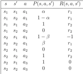
3.2 A simple environment of two states (plot taken from [2]). . . 57

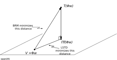
3.3 LSTD fixed-point. Φw lies on the hypothesis space _F spanned by the columns of Φ (i.e., span(Φ)). However, when apply-ing the Bellman operator T, T(Φw) does not necessarily lie onto span(Φ). Hence, LSTD first minimizes the distance _kT(Φw) ₋

y_k, for anyy _{∈ F},yielding the projectionΠT(Φw)ontospan(Φ), and then minimizes_kΦw−ΠT(Φw)_k. On the other hand, Bellman Residual Minimization (BRM) minimizes_kΦw₋T(Φw)_kdirectly, however, this optimization problem does not reduces to the fixed-point problem of TD learning (for more details on BRM see [3]) —plot taken from [4]. . . 67

(18)

3.4 (a) Averaged approximation error over50trials forV function using 1365 features versus samplesm. As shown both methods perform similarly when samples are collected on-policy. (b) Averaged ap-proximation error over50trials forQfunction using2728features versus samples m. ADMM-TD is able to offer better approxima-tions for Q function when samples are collected off-policy since LARS-TD, in order not to violate the optimality conditions, incor-porates also an`2regularization (elastic net). . . 82 3.5 (a)10-fold cross-validation (CV) versus regularization parameterλ;

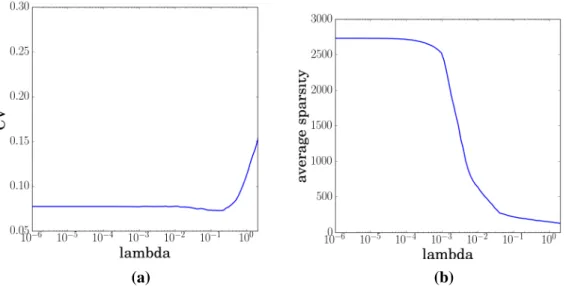
minimum CV achieved forλ= 0.214. (b) averaged sparsity versus regularization parameter λ; λ = 0.214 yields approximately 227 nonzero features. . . 83

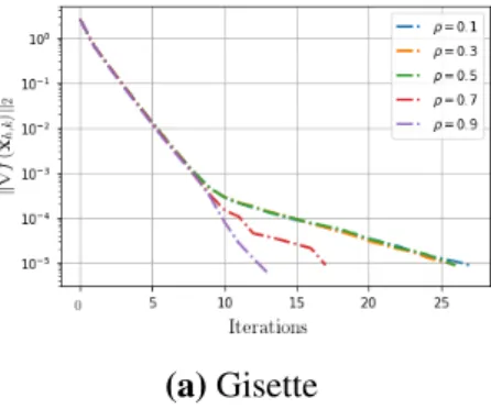
4.1 Behavior of YAWN for different values ofρ1. . . 146 4.2 Experiment of different algorithms over various datasets. Error vs

(19)

List of Tables

3.1 Recycling Robot: Transition probabilities and expected rewards. . . 58 3.2 Mean simulated reward (20 trials) _± standard error between

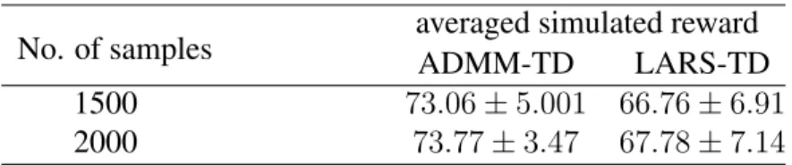
ADMM-TD and LARS-TD for m = (1500,2000) samples and 2728features —the larger the averaged simulated reward the better the policy is. ADMM-TD yields better policies compared to the elastic net formulation of LARS-TD. . . 84

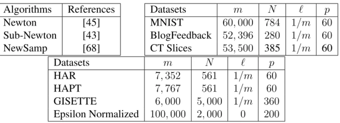
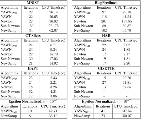
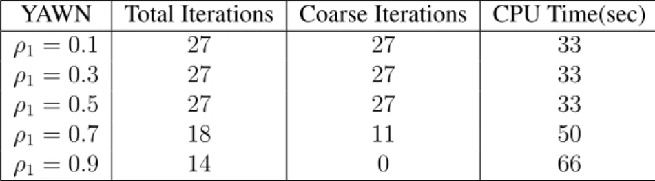
4.1 Datasets and Algorithms used in the experiments, available from https://www.csie.ntu.edu.tw/\protect\unhbox\ voidb@x\penalty\@M\{}cjlin/libsvmtools/datasets/ andhttp://archive.ics.uci.edu/ml/index.php . . . 143 4.2 Comparison of optimization algorithms over various datasets. . . 144 4.3 Comparison of YAWN of different values inρ1on Gisette dataset. . 145

(20)

(21)

Introduction

“There are reasons to be sad, disconsolate, bitter, but there is not a single reason to be hopeless.”

Nazim Hikmet Ran

Modern machine learning applications often require optimizing large-scale mod-els. In this domain, the ability to obtain sufficiently accurate solutions quickly is crucial. Examples of such problems can be found in [5, 6, 7, 8]. In the context of computational optimization, there have been many developments for reducing the computational burden of solving large-scale optimization problems. In general, for an arbitrary optimization problem, aiming for extremely fast convergence rates is typically a very difficult task [9]. Therefore, much emphasis has been given in designing methods that take advantage of the problem structure. In addition to the fast solvers, the goal of accuracy in prediction is equally important. For this reason, exploitation of the prior knowledge about regularity in datasets, such as sparsity and smoothness, has become necessary. In particular, regularization in statistical regres-sion setting has attracted an increasing interest during the last decade. Statistical regularization, or alternatively, penalization of the standard least-squares problem, has been efficiently applied in many diverse fields, such as classification, prediction on multivariate datasets (eg., graphical models), image and signal processing and

(22)

compressive sensing. To this end, the goal of this thesis is to develop and study optimization methods that take advantage of the structures of optimization models that arise in machine learning applications.

1.1

ADMM for Reinforcement Learning

Problems with large datasets are encountered in almost all applied fields such as AI, statistics, machine learning, etc. Here, we discuss Alternating Direction Method of Multipliers (ADMM), a general optimization framework which has recently re-ceived a lot of attention for various large regularized regression problems [10, 11]. ADMM is most useful when applied to optimization problems with a separable ob-jective function. Regularized regression problems, such asLasso, ridge regression and basis pursuit, fall into this category. In particular, since the function subject to minimization is separable, it can be split into two parts, and thus the algorithm can handle each part completely separately (i.e., each iteration can be viewed as an independent subproblem). For instance, each ADMM iteration implies a small convex optimization problem for which is often the case that it can be calculated analytically, thus yielding an efficient algorithm in terms of time complexity. The algorithm was developed in 1970s and is closely related to algorithms such asDouglas-Rachford splitting, Dykstra’s alternating projections and the method of multipliers [12]. ADMM has a fairly well established theory in the context of con-vex optimization and hence, within this domain, it has found numerous applications in different fields such as in [13] for compressive sensing, [14] for graphical mod-els and [15] for signal processing and control problems. However, convexity of the objective functions does not always hold in many applied fields. For instance, the Reinforcement Learning problem we discuss below considers solving a fixed-point problem which in turn does not correspond to any other convex optimization problem.

(23)

Reinforcement Learning

Reinforcement Learning (RL) is a sub-field of machine learning [16]. As the name suggests, it considers learning problems where, when interacting with the environ-ment, we learn what to do or what actions to take in order to optimize the desirable outcome. In particular, RL considers an agent which interacts with the environment. The agent finds itself in a current state and faces the dilemma of what action to se-lect, since it is not told which action performs optimally. Moreover, after executing an action, the environment returns a new state together with a reward (indicating how good the selected action was) and the procedure continues in the same manner. In practice, we face problems where a sequence of actions (policy) needs to be taken in order to achieve our goal. The desirable outcome (or goal) in RL is to maximize the sum of the expected reward, or equivalently, to find the assignment of actions to each state that, when executed, maximizes the sum of the expected reward (optimal policy).

Furthermore, RL can be considered as a part of Artificial Intelligence(AI) and as such it aims for autonomous systems (or intelligent agents) that can make decisions and eventually achieve the determined goals. During the last years RL has success-fully found many applications in AI such as robotics [17], autonomous helicopter [18] andTD-Gammon[19]. It has also been applied in fields such as Control the-ory and Operational Research (inverted pendulum [20] and shop scheduling [21], respectively).

Here, we consider off-line (batch) RL [22] where the agent is not allowed to interact with the environment in order to obtain the optimal policy but instead is given a fixed set of sampled states and actions, typically finite. Using the given information, the agent forms a random policy which is then used to interact with the environment; the policy is fixed and does not improve during the procedure. Hence, the goal in off-line RL is, given the existing data, to find the policy that maximizes the sum of rewards. The goal of maximizing the sum of rewards can be attained by computing the so called value functions.

(24)

A core problem in off-line RL emerges in situations where the state space is large, where explicit computation of the value functions becomes infeasible. Instead, ap-proximation techniques provide the only way forward. In this work we are inter-ested in linear representation of the value functions since the updates reduce to a simple form when employing first- or second-order methods [23, 16]. Least-squares and regularized least-Least-squares methods have been proposed to solve the RL problem [24, 25, 26, 3, 27, 28, 29, 30, 31]. However, none of the proposed meth-ods have been able to solve the RL problem, especially when the goal is to find the optimal policy. In particular, least-squares methods are known to be vulnerable to over-fitting and thus lead to poor predictions. On the other hand, `1-regularized least-squares methods, although have been found to overcome the over-fitting issue, only converge under some strong assumptions that rarely hold in practice.

In this thesis, we propose to use ADMM for solving the`1-regularized least-squares optimization problem. This problem, however, reduces to a fixed-point problem and as such it does not correspond to any convex optimization problem. Therefore, we modify the standard ADMM in order to now solve the aforementioned fixed-point problem. Our theoretical analysis shows that our proposed method is able to return efficient solutions. Incorporating`1-regularization into the fixed-point so-lution means that the underlying optimization problem is separable and thus can be handled efficiently by ADMM producing fast iterations. Another advantage is that ADMM yields closed-form solutions for the subproblems of the`1-regularized least-squares problem that are easy to compute. However, since the optimization problem we consider here is not convex, a proof of convergence is a difficult task and remains open. Finally, we perform preliminary numerical experiments which indicate the effectiveness of our proposed method.

The main contributions of this work have been published in:

Nikos Tsipinakis and James D.B. Nelson. Sparse temporal difference learning via alternating direction method of multipliers. InMachine Learning and Applications (ICMLA), 2015 IEEE 14th International Conference on, pages 220–225. IEEE,

(25)

2015.

1.2

Multilevel Methods

Multilevel methods in optimization arise from the general field of multigrid meth-ods that were first introduced for solving (non-)linear Partial Differential Equations (PDEs) [33, 34, 35, 36]. In this domain, multigrid methods, in order to overcome the computational burden, attempt to offer approximate solutions from coarser dis-cretizations of a mesh. They construct a hierarchy of different-sized discretization problems where the idea is to use the information of the smaller problems (in lower dimensionality) to solve the exact problem. Problems of lower dimensions are often calledcoarseproblems. The advantage of this procedure is clear: coarse problems are typically much easier to be optimized because of their significantly reduced di-mensionality; we note that, directly solving for the exact solution in the context of PDEs is expensive.

When the discussion comes to the context of large-scale optimization in machine learning applications the situation is similar: optimizing the exact model is often an intractable task (see [8] for examples in applications such as background extraction in video processing, and face recognition). To this end, the multigrid idea (solving coarse models in order to obtain a solution of the exact model) was introduced into optimization where many authors adopted the namemultilevel[37, 38, 39, 40]. Importantly, the performance of multilevel methods has been found very efficient and in many cases it has been shown to outperform classical optimization methods. Classical optimization methods such as first order methods, stochastic, proximal, accelerated or otherwise, are the most popular class of algorithms for the large-scale optimization models that arise in modern machine learning applications. The ease of implementation in distributed architectures and the ability to obtain a reason-ably accurate solution quickly are the main reasons for the dominance of first-order methods in machine learning applications. In the last few years, second-order

(26)

meth-ods based on variants of the Newton method have also been proposed. Second-order methods, such as the Newton method, offer the potential of quadratic convergence rates (the holy grail in optimization algorithms). Unfortunately, the conventional Newton method has huge storage and computational demands and does not scale to applications that have both large and dense Hessian matrices. To improve the con-vergence rates, and robustness of the optimization algorithms used in machine learn-ing applications many authors have recently proposed modifications of the classical Newton method [41, 42, 43, 44]. However, the current state-of-the-art methods dis-cussed previously suffer from either of the following shortfalls:Shortfall I:Lack of scale-invariant convergence analysis without restrictive assumptions, and, Short-fall II:Lack of global super-linear rates without ad-hoc assumptions regarding the spectral properties of the input data.

In this thesis, we propose a general unconstrained optimization method based on the multilevel framework and we attempt to address both shortcomings listed above. Our theoretical analysis is based on the theory of self-concordant functions and we are able to prove a super-linear convergence rate without relying on unknown pa-rameters (scale invariant analysis). Thus, we argue that with the results presented in this thesis, the theory of the variants of the Newton methods can be considered to be on-par with the theory of the classical Newton method. These fundamental results are achieved by drawing parallels between the second-order methods used in machine learning, and the so-called Galerkin model from the multilevel optimiza-tion literature. To the best of our knowledge, this is the first multilevel optimizaoptimiza-tion method that captures the advantages of the multigrid theory (i.e., fast global con-vergence rates) and in parallel does not suffer from either of the shortfalls listed above.

The main contents of this work are currently in preparation with title:

Nikos Tsipinakis and Panos Parpas. Exploiting coarse-grained models for faster, scale-invariant convex optimization.

(27)

Background Theory

In this chapter we present the most relevant theory of optimization methods required for this thesis. In particular, in the first section we present the theory of convex and self-concordant functions. In the second section, we review the most relevant first-and second-order methods for unconstrained convex optimization. In the third, we present the Alternating Direction Method of Multipliers and we describe the setting of the equality constrained convex optimization. In section four, we present opti-mization methods for approximating matrices with low-rank structure. We would like to emphasize that the goal of this chapter is not to provide a complete review of the methods that will be discussed. Our purpose, nevertheless, is to provide the reader with the necessary theoretical knowledge required before moving forward to the core of this work.

2.1

Preliminaries

In this section we collect some general, fundamental, results that will be useful throughout this thesis.

For anyx,y_∈_Rnthe standard inner product is defined by

hx,y_i=xTy=

n

X

i=1

(28)

A function f : _Rn _→

R is said to be proper when domf 6= ∅, wheredomf =

{x_∈_Rn _: _f₍_x₎_<₊_∞}_{. Additionally, a function}_f _:

Rn→Ris said to be closed when its epigraph,epif, is a closed set, where

epif =_{(x, t) : x_∈domf, t∈R, f(x)≤t}.

A function f : _Rn _→

R+ is called a norm if for any x,y ∈ Rn we have that: (i)

f(x) = 0, thenx = 0; (ii)f(λx) =_|λ|x, λ∈ R; (iii) the triangle inequality holds, i.e.,f(x+y)_≤f(x) +f(y). A vector space_Hwith a norm that satisfies the above conditions is called a normed vector space. Let p ≥ 1. The`p-norm is defined as

follows kx_kp = n X i=1 |xi|p !1_p .

Let _H = (_H,_{k · k})be a normed vector space. A mapping f : _{H → H} is called contraction if for anyx,y_{∈ H}andγ ∈(0,1)we have that

kf(x)₋f(y)_{k ≤}γ_kx₋y_k.

The Banach space is defined as a complete normed vector space, where every Cauchy sequence is convergent (i.e., lim

n→∞_msup_≥_nkan −amk = 0, where {an}n≥0 is

a sequence on_H).

Theorem 2.1.1 (Banach’s fixed-point theorem [1]). LetV be a Banach space and

T :V →V be a contraction mapping. ThenT has a unique fixed-point.

For more details on the preliminary theory discussed above see [45, 46, 1].

2.1.1

Convex Functions

A functionf : _Rn_→

Ris convex, if, for all x,y∈ domf and someθ ∈[0,1], we have that

(29)

wheredomf is a convex set. Based on the first-order information, for a differen-tiable functionf, the above definition becomes

f(y)_≥f(x) +_∇f(x)T(y₋x). (2.1) Inequality (2.1) constitutes a necessary and sufficient condition for a functionf to be convex. Further, a function is called strictly convex if (2.1) holds with strict inequality. Importantly, note that if _∇f(x)T = 0 then we havef(x) _≤ f(y)for all x,y _∈ domf which means that x is global minimizer of f. In addition to the first-order convexity condition, the second-order condition, assuming a twice differentiablef is given by

∇2

f(x)0,

for allx _∈ domf. In other words, a twice differentiable function is convex when the Hessian matrix is positive semi-definite. If, in addition, the Hessian matrix is positive definite thenf is strictly convex.

A twice differentiable is strongly convex if there exists a constantµ >0such that

∇2_f₍_x₎

µIn×n, (2.2)

where In×n is the identity matrix. A direct consequence of strong convexity is

that the Hessian matrix is also bounded above, i.e., there exists M > 0 such that

∇2_f₍_x₎_M_I

n×n. Combining both bounds of the Hessian matrix we have that

f(x)+_∇f(x)T(y₋x)+µ 2ky−xk2 ≤f(y)≤f(x)+∇f(x) T₍_y −x)+M 2 ky−xk2. (2.3) For a more refined analysis on convex functions we refer the reader to [45, 9].

2.1.2

Self-Concordant Functions

In this section we recall some of the main properties and inequalities of the class of self-concordant functions. We follow similar notation as in the books [9, 45] (for a

(30)

complete theory on self-concordant functions see [9]).

A univariate convex functionφ:_R_→_Ris called self-concordant if

|φ000(x)_{| ≤}2φ00(x)3/2. (2.4) Examples of such functions include but not are limited to linear, quadratic and logarithmic. Further, consider a multivariate function f : _Rn _→ _R and also fix x _∈ domf and a direction u _∈ _Rn_{. Then,} _φ₍_t_{) =} _f₍_x ₊_t_u₎ _{is called}

self-concordant for all xand u if it is self-concordant along every line in its domain. Importantly, self-concordance is preserved under composition with any affine func-tion.

Next, givenx_∈domfand assuming that_∇2f(x)is positive-definite we can define the following norms

ku_kx =h∇2f(x)u,ui1/2 and kvk∗x =h[∇ 2

f(x)]−1v,v_i1/2, (2.5) where it holds that_|hu,v_{i| ≤ k}u_k∗_x_kv_kx. The Newton decrement is defined as

λf(x) = k∇f(x)k∗x=k[∇ 2

f(x)]−1/2_∇f(x)_k2. (2.6) In addition, we take into consideration two auxiliary functions, both introduced in [9]. Define the univariate functionsωandω∗such that

ω(x) =x−log(1 +x) and ω∗(x) =₋x−log(1₋x), (2.7)

with domω = _{x _∈ R : x ≥ 0} and domω∗ = {x ∈ R : 0 ≤ x < 1}, respectively. Note that both functions are convex and their range is the set of positive real numbers.

(31)

Now, from the definition (2.4), we have that d dt φ 00 (t)−1/2 ≤ 1,

from which, after integration, we obtain the following bounds

φ00₍₀₎ (1 +tφ00₍₀₎1/2₎2 ≤φ 00 (t)_≤ φ 00₍₀₎ (1₋tφ00₍₀₎1/2₎2 (2.8) where the lower bound holds fort_≥ 0and the upper bound fort _∈[0, φ00₍₀₎−1/2_), with t _∈ domφ. Consider now functions on _Rn. For x _∈ domf, and for any y_∈S(x), whereS(x) =_{y_∈_Rn_:_k_y₋_x_k x<1}, we have that (1_{− k}y₋x_kx)2∇2f(x) ∇2f(y) 1 (1_{− k}y₋x_kx)2∇ 2_f₍_x₎_. (2.9)

Finally, let us state one last pair of inequalities that will be useful in our analysis. Forxandyfromdomf it holds that

f(y)_≥f(x) +_h∇f(x),y₋x_i+ω(_k∇f(y)_{− ∇}f(x)_k∗_y)

and if also_k∇f(x)_{− ∇}f(x)_k∗_y<1, then

f(y)_≤f(x) +_h∇f(x),y₋x_i+ω∗(_k∇f(y)_{− ∇}f(x)_k∗_y). (2.10)

For more details on self-concordant functions see [45, 9].

2.2

Unconstrained Convex Optimization Methods

In this section we are interested in solving the following unconstrained optimization problem

min x∈Rn

f(x), (2.11)

where f : _Rn _→

R is a convex function. Further, we assume that f is twice differentiable and a minimizerx∗exists. In the unconstrained case,x∗is an optimal

(32)

Algorithm 2.1Gradient Descent 1: Initialize:x0 ∈Rn

2: fork = 0,1, . . .do

3: Compute the direction asdk=−∇f(xk)

4: Choosetkthrough inexact line search Algorithm 2.2

5: Update

xk+1 :=xk+tkdk

6: end for 7: return xh,k

point if and only if

∇f(x∗) = 0. (2.12) Therefore, the goal is to seek points that satisfy (2.12). In practice, this can be achieved via an iterative scheme by producing a sequence ofk points; the iterative procedure terminates, at some iteration k, if _k∇f(x)_k2 < , for some tolerance

>0.

2.2.1

Gradient Descent Method

In this section we discuss first-order methods for solving the convex program (2.11). Specifically, we will concentrate on the gradient descent method [46, 45, 9], a method which is frequently well suited to large-scale optimization problems since, by definition, it uses “cheap” iterations based on the first-order information (i.e., gradients) of the objective function.

Consider the optimization problem in (2.11). The gradient descent method builds iterates using the first-order information. In particular, the negative gradient is cho-sen as search direction, that is, dk = −∇f(xk), and thus we take the following

iterative scheme

(33)

Algorithm 2.2Armijo Rule

1: Input: α _∈(0,0.5), β _∈(0,1)and a descent directiond 2: t:= 1

3: whilef(x+td)> f(x) +αt∇f(x)Tddo 4: t:=βt

5: end while

This choice of search direction produces a descent algorithm since

∇f(xk)dk =−k∇f(xk)k2 <0

which means that, at each iteration, we expectf(xk+1) < f(xk), unlessxk is

op-timal. The gradient descent method has been analyzed assumingf is am-strongly convex function and enjoys a linear convergence rate. In Algorithm 2.1, the step size is computed through the inexact line search method. If we instead assume that

f has aL-Lipschitz continuous gradient, withLknown, then we can use constant step size ast = 1/L(similarly, when assumingm-strongly convex function, there exists parameterMsuch that the constant step yieldst= 1/M). Since in most prac-tical problems such constants are typically unknown, for computingtk, we consider

the Armijo rule or inexact line search method, see Algorithm 2.2.

2.2.2

Newton Method

In this section we consider the Newton method [46, 45, 9], a second-order method for solving (2.11). In general, second-order methods make use of the information which emerges from the second derivative of the objective function. We discuss the Newton method with analysis based on both classical theory (Lipschitz continuity and strongly convex functions) and theory of self-concordant functions.

We are interested in solving the convex optimization problem (2.11). The Newton method builds the iterates based on the second-order Taylor approximation of f, i.e., f(xk+d)≈f(xk) +h∇f(xk),di+ 1 2d T ∇2 f(xk)d.

(34)

Algorithm 2.3Newton Method 1: Initialize:x0 ∈Rn

2: fork = 0,1, . . .do

3: Compute direction and decrement by

dk =−[∇f(xk)]−1∇f(xk), λ(xk)2 =∇f(xk)T[∇2f(xk)]−1∇f(xk)

4: Choosetkthrough inexact line search Algorithm 2.2

5: Update

xk+1 :=xk+tkdk

6: end for 7: return xh,k

Since_∇2_f₍_x

k)is positive definite, we can minimize the right-hand side (which is a

convex quadratic function) to obtain the Newton direction

dk =−[∇2f(xk)]−1∇f(xk).

Positive definiteness of _∇2f(xk) also implies that the Newton step is a descent

direction

∇f(xk)Td=−∇f(xk)T[∇2f(xk)]−1∇f(xk)<0 (2.13)

unless xk is a minimizer. It is easy to see that dk is what we need to add to the

current pointxkso that to minimize the right-hand side of the Taylor approximation.

The intuition indicates that if f in (2.11) is a quadratic function, then the point xk+dkis exactly the minimizer offand thus the Newton method converges in one

iteration. Relation (2.13) leads us to the definition of the Newton decrement

λ(xk) =

∇f(xk)T[∇2f(xk)]−1∇f(xk)

1/2

.

The Newton decrement plays important role in the analysis of the Newton method and can be used as an exit condition (i.e.,λ(xk)2/2≤for some small >0).

One important aspect of the Newton method is that the Newton step builds iterates that are invariant of affine transformation of variables. This means that the conver-gence rate is not affected by the input data.

(35)

Analysis with classical theory

In addition to the basic assumptions (convexity and twice differentiable function), the analysis of the Newton method has been conducted by further assuming the following

Assumption 2.2.1. Functionf is strongly convex. Then, there exist positive con-stantsmandM such that

mIn×n≤ ∇2f(x)≤MIn×n.

whereIn×nis the identity matrix. Further,f possessesL-Lipschitz continuous

Hes-sian, i.e.,

k∇2_f₍_x₎

− ∇2_f₍_y₎

k2 ≤Lkx−yk, x,y∈domf.

The above assumption is typical when analyzing descent methods based on second-order information. It has been proved that the Newton method can achieve quadratic convergence rate. In particular, convergence is split into two phases according to the magnitude of_k∇f(xk)k2: (a) the damped Newton phase where Algorithm 2.3 can choose step sizetk < 1 and (b) the quadratic phase where the convergence is

extremely fast and the step is always chosen astk= 1.

Theorem 2.2.2([45]). Suppose that Algorithm 2.3 is performed and let Assumption 2.2.1 hold. There existsη_∈(0, m2_/L_]_{such that}

1. if_k∇f(xk)k2 > η, then there existsγ =αβ_Mm2 such that

f(xk+1)−f(xk)≤ −γ 2. if_k∇f(xk)k2 ≤η, thentk = 1and k∇f(xk+1)k2 ≤ L 2m2 (k∇f(xk)k2) 2

(36)

Theorem 2.2.2 describes the convergence behavior of the Newton method. If the current point xk is far from the optimizer, then the damped Newton phase is

per-formed which guarantees reduction of the value function according to some constant

γ.Ifxkis sufficiently close to the minimizer, then we obtain quadratic reduction in

the value of_k∇f(xk+1)k2.

Although the Newton method, under Assumption 2.2.1, achieves quadratic conver-gence rate, we cannot say much about both regions of converconver-gence since constants

Landmare typically unknown in practice. Intuition suggests that sufficiently small values inLyield extremely fast reduction in_k∇f(xk+1)k2. In the next section we see how to obtain explicit expressions about the quadratically convergence phase of Newton method.

Analysis with self-concordant functions

The analysis of the Newton method conducted in the previous section has two im-portant shortcomings: (a) complexity bounds involve constantsm, M andLwhich are typically not known in practice and thus we cannot obtain an explicit bound on the number of iterations; (b) Although the Newton step produces an affine invariant method with respect to the change of coordinates, its analysis is not affine invari-ant, i.e., if we change coordinates all constantsm, M andLchange. Therefore we should seek a theory that is independent of the affine transformation of variables. The way forward for achieving this goal is to replace Assumption 2.2.1 with the elegant theory of self-concordant functions.

Therefore, we are interested in solving the optimization problem (2.11) where, now, we assume that the objective functionf is a strictly self-concordant function. The idea of the analysis of Newton method remains the same but now the results do not depend on any unknown constants. In contrast to the classical analysis, the region of quadratic convergence depends on the magnitude of the Newton decrement (in place of the norm of the gradient).

(37)

Theorem 2.2.3 ([45]). Suppose that Algorithm 2.3 is performed and let f be a strictly self-concordant function. Then, forη∈(0,1/4],

1. ifλ(xk)> η, then there existsγ =αβη2 η

2

1+η such that

f(xk+1)−f(xk)≤ −γ

2. ifλ(xk)≤η, thentk= 1and

λ(xk)≤2λ(xk)2

Theorem 2.2.3 shows that the Newton method enjoys a quadratic convergence rate. In particular, we come up with an explicit expression of the region of the quadrat-ically convergent phase (independent of any unknown constants). This mean that Algorithm 2.3 is affine invariant with respect to the change of coordinates.

To this end, the Newton method, either analyzed using the classical theory or the theory of self-concordant functions, has been found to outperform many algorithms due to its quadratically convergent phase. However, the main drawback arises in large-scale optimization problems since handling _∇2_f₍_x₎ _{is typically infeasible.} On the other hand, for moderate-sized optimization problems, Newton method can be considered as one of the best method to be applied to, due to its extremely fast convergent behavior and its advanced theoretical analysis.

2.3

Equality Constrained Convex Optimization

Consider the optimization problem of the form minimize

x∈_Rn f(x)

subject to Ax=b,

(38)

where A _∈ _Rm×n_, _x _∈

Rn, b ∈ Rm and f : Rn → R is a convex function with primal optimal valuep∗_{. The Lagrangian [46, 10, 11, 45] associated with the}

problem (2.14) is a functionL:_Rn_×

Rm →Rdefined as

L(x,y) = f(x) +yT(Ax₋b),

wherey_∈_Rm _{is called the dual variable or the Lagrange multiplier of the equality}

constraint. The Lagrange dual function g : _Rm _→ _R is defined as the infimum of the Lagrangian, that is

g(y) = inf

x∈_Rn{f(x) +y

T

(Ax₋b)_}.

There are two important properties regarding the Lagrangian. First, the dual func-tion,g(y), is always concave —this is true even in the case where the optimization problem (2.14) is not convex. Moreover, it implies lower bounds on the primal optimal valuep∗

, for anyy_∈_Rm, i.e.,

g(y)_≤p∗.

Therefore, this leads one to search the best available lower bound. The best bound can be obtained by the following unconstrained optimization problem, called the Lagrange dual problem

max y∈Rm

g(y). (2.15)

We denote the dual optimal value of the above optimization problem asd∗_{. Note that}

(2.15) is always convex since it is a maximization problem over a concave function. When the best lower bound obtained by the dual problem is equal to the primal optimal value of the initial problem, i.e.,d∗ ₌_p∗

, we say either that the duality gap is zero or that strong duality holds.

(39)

KKT Optimality Conditions

We shall now examine the sufficient and necessary conditions of the problem (2.14). Considerx∗andy∗as the primal and dual optimal points, respectively, and also that strong duality holds. We have the following optimality conditions associated with the optimization problem (2.14) and its dual problem (2.15)

∂f(x∗) +ATy∗ ₃0 Ax∗ =b.

The above optimality conditions are calledKarush-Kuhn-Tucker(KKT) conditions. Anyx∗andy∗must satisfy the above conditions when duality gap is zero [45]. Note that the first equation is obtained by taking the gradient of the Lagrangian overxand the second equation because of the fact that the equality constraint must always hold. The operator ∂ denotes the subdifferential of a function since f(x) might not be differentiable. Additionally, ∂f is set-valued and hence we use _∈ instead of=. Whenf(x)is differentiable, the subdifferential symbol,∂, can be re-placed by the gradient, and the inclusion symbol by equality (for more background on subdifferential calculus see [47]).

Augmented Lagrangian

Consider now the optimization problem of the form minimize x∈Rn f(x) + ρ 2kAx−bk 2 subject to Ax=b. (2.16)

For any feasible pointx, the above optimization problem is equivalent to (2.14) — the term ρ₂_kAx₋b_k2 will be equal to zero. Therefore, the Lagrangian of (2.16) is

Lρ(x,y) =f(x) +yT(Ax−b) +

ρ

2kAx−bk 2

(40)

where ρ > 0 denotes the penalty parameter. Equivalently, equation (2.17) can be viewed as theaugmented Lagrangianof the problem (2.14) [10, 11]. Note that for

ρ= 0the augmented Lagrangian yields the standard Lagrangian.

2.3.1

Alternating Direction Method of Multipliers

In this section we discuss problems of the form as in (2.14) where the objective func-tion is separable, i.e., f(x) = g(x) +h(x). The Alternating Direction Method of Multipliers (ADMM) is a simple but powerful algorithm as it has been demonstrated to be very efficient for problems with separable objective functions in the context of large scale optimization [10, 11]. Consider the following composite problem

minimize

x∈_Rn h(x) +g(z)

subject to Ax+Bz=c,

(2.18)

where A _∈ _Rm×n_, _x _∈

Rn, B ∈ Rm×p, z ∈ Rp and c ∈ Rm. Moreover, func-tionsh andg are convex, proper and closed functions. The variablez emerges by performing variable splitting over x, i.e., xhas been split into two parts, namely xandz, and then, for feasibility purposes, we must incorporatezinto the equality constraint.

The augmented Lagrangian associated with the problem (2.18) is of the form

Lρ(x,z,y) =h(x) +g(z) +yT(Ax+Bz−c) +

ρ

2kAx+Bz−ck 2_,

wherey _∈ _Rm _{denotes the dual variable and}_{ρ >} ₀_{is the penalty parameter. The}

ADMM iterations are functions of the augmented Lagrangian andρcan be consid-ered as the step-size parameter of the algorithm. In particular, we have the following

(41)

ADMM iterations xk+1 := argmin x∈Rn {Lρ(x,zk,yk)} zk+1 := argmin z∈Rp {Lρ(xk+1,z,yk)} yk+1 :=yk+ρ(Axk+1+Bzk+1−c). (2.19)

The above iterations are often difficult to calculate and thus is more convenient to express the Lagrangian in the following form

Lρ(x,z,y) = h(x) +g(z) +yT(Ax+Bz₋c) + ρ 2kAx+Bz−ck 2 ₌ h(x) +g(z) +yT(Ax+Bz₋c) + ρ 2kAx+Bz−ck 2₊ 1 2ρkyk 2₋ 1 2ρkyk 2 ₌ h(x) +g(z) + ρ 2(kAx+Bz−ck 2₊2 ρy T₍_Ax₊_Bz −c) + 1 ρ2kyk 2₎ − 1 2ρkyk 2 ₌ h(x) +g(z) +_kAx+Bz₋c+ 1 ρyk 2₋ 1 2ρkyk 2 ₌ h(x) +g(z) +_kAx+Bz₋c+u_k2₋ ρ 2kuk 2_,

whereu _∈ _Rm denotes the scaled dual variable, u = 1_ρy. Hence, by replacing the above result in (2.19), we have that

xk+1 := argmin x∈Rn {h(x) + ρ 2kAx+Bzk−c+ukk 2 } zk+1 := argmin z∈Rp {g(z) + ρ 2kAxk+1+Bz−c+ukk 2 } uk+1 :=uk+Axk+1+Bzk+1−c. (2.20)

As a result, both ADMM forms, (2.19) and (2.20), are equivalent and also it is evi-dent that the right hand side of the latter ADMM form can be often easily evaluated since the minimization part is simpler (easier differentiation of such a function) —this form is also called as scaled form due to the scaled dual variableu.

(42)

Optimality Conditions and Convergence

At the optimal pointsx∗, z∗ andy∗, ADMM must satisfy the following optimality conditions

Ax∗+Bz∗₋c= 0 (2.21)

∂h(x∗) +ATy∗ ₃0 (2.22)

∂g(z∗) +BTy∗ ₃0. (2.23) It has been shown that the optimality conditions associated with the ADMM itera-tions (2.19) are

0_∈∂h(xk+1) +ATyk+1+ρATB(zk−zk+1) (2.24) 0_∈∂g(zk+1) +BTyk+1. (2.25) For more details on the derivation of the aforementioned optimality conditions see [10]. It is obvious that equation (2.25) always satisfies optimality condition (2.23). On the other hand, equation (2.22) will only be satisfied when

ρATB(zk+1−zk)∈∂h(xk+1) +ATyk+1.

The quantity on the left-hand side of the above relation is called the dual residual and we define

qk+1 =ρATB(zk+1−zk).

Furthermore, optimality conditions (2.21) indicate that

Axk+1+Bzk+1−c= 0, which is called primal residual, and thus we define

(43)

ADMM has been shown to converge under the most general assumptions. In partic-ular, the extended functionsh:_Rn_→

R∪ {+∞}andg :Rp →R∪ {+∞}need to be convex, proper and closed functions and moreover the standard Lagrangian (L0) to have a saddle point, i.e.,

L(x∗,z∗,y)_≤L(x∗,z∗,y∗)_≤L(x,z,y∗).

Note that functionshandg can take the value+_∞and also that there no assump-tions on matrices A and B. Under these assumptions it has been proved that the algorithm converges to the optimal solutionp∗_{and, further, the dual variable}_y_{to its}

optimal pointy∗_as_k

→+_∞. Additionally, it has been shown that both primal and dual residuals converge to zero in the limit.

2.3.2

Proximal ADMM

In this section we discuss the proximal form of ADMM. We start by providing the relevant theory on proximal operators.

The proximal operator of a convex, proper and closed functionf :_Rn _→

R∪{+∞} is defined as prox_µf(v) = argmin x∈_Rn {f (x) + 1 2µkx−vk 2_}_, whereprox_µf : _Rn _→

Rn [11]. Moreover,µ > 0denotes the step-size parameter indicating how fast we want to move towards the optimal point.

The resolvent of an operator H with scalar µ is defined as JµH = (I+µH)−1 —note that the resolvent is a relation (for more details see [48]). In the case of proximal operators, we have that the resolvent of the subdifferential operator and the proximal operator coincide, so we have that

prox_µf =Jµ∂f.

(44)

the resolvent of the subdifferential is single-valued even though ∂f is set-valued. Furthermore, the application of the proximal operator can be viewed as a fixed-point iteration. In particular, it has been shown that for any maximal monotone operatorH, xminimizesH, i.e., 0 _∈ H(x), if and only ifx = JµH(x), which in turn yields

0_∈∂f(x) _⇔ x=prox_µf(x). (2.26) For a proof of the theorem and details on monotone operators see [12]. As a result, equation (2.26) implies theproximal point algorithm, that is

xk+1 :=proxµf(xk).

The proximal point algorithm has not been found effective in most applications since it requires minimization over f(x) + ₂1_µ_kx₋v_k2 _{at each iteration. For this} reason, it is more useful to apply either proximal gradient method or ADMM in its proximal form, also known asDouglas-Rachford splitting method. The former method considers the unconstrained optimization problem of the form

minimize x∈Rn

h(x) +g(x), (2.27)

where, again, the objective function f has been split into h and g and moreover we require h to be differentiable. The proximal gradient method consists of the following iterations

xk+1 :=proxµkg(xk−µk∇h(xk)),

whereµk>0denotes the step-size parameter. It has been shown that the algorithm

also converges for a fixed step-size, µ, and moreover, in the case where_∇h isL -Lipschitz continuous, µ can take values in (0, 2

L] (for more discussion about the

proximal gradient method and its accelerated form see [11]).

(45)

unconstrained problem (2.27)

minimize h(x) +g(z) subject to x=z,

where we now introduce the equality constraint requiring variables xand z to be equal. Thus, we have the following iterations

xk+1 := proxµh(zk−uk)

zk+1 := proxµg(xk+1+uk)

uk+1 := uk+xk+1−zk+1, wherex,z,u_∈_Rn_{, with}_u_{denoting the dual variable.}

The advantage of ADMM against the proximal gradient method is that the former evaluates h(x) and g(z) completely separately, in many cases, yielding the algo-rithm to perform more efficiently in terms of time complexity. Additionally, none of the functions h(x) andg(z)are required to be differentiable. Finally, it is easy to see that, by replacingu = 1_ρy, µ = 1_ρ and matrices A,B with the identity ma-trix, the ADMM version in (2.19) is equivalent with the proximal version presented above, and thus proximal ADMM can be viewed as a special case of the standard ADMM in Section 2.3.1.

2.4

Low-Rank Approximation Methods

A key feature in modern (large-scale) machine learning problems is the limitation of storing excessively big matrices. Fortunately, in many applications (see [49] and references therein), these matrices exhibit a low-rank structure. First, consider a generalA_∈_Rn×m_{matrix. The Singular Value Decomposition of}_A_{is summarized}

in the following theorem.

(46)

ex-ist unitary matrices U _∈ _Rn×n _and _V _∈

Rm×m and a diagonal matrix Σn =

diag(σ1, . . . , σn)withσ1 ≥σ2 ≥ · · · ≥σn>0such that

A=UΣV, Σ=Σn 0

whereΣis a diagonaln×mmatrix.

The positive constants σ1, . . . , σn are called the singular values of A and when

rank(A) = n they coincide with the square roots of the eigenvalues of the matrix AAT_{. If, further, matrix} _A _{is known to be of} _rank-_{p < n}_{, the above theorem}

applies with singular values ofΣnbe asσ1 ≥ · · · ≥σp >0 = σp+1 =· · ·=σn.

For the purposes of this work, we consider low-rank approximations of a positive semi-definite matrix A _∈ _Rn×n_{. We can obtain an rank-}_p _{approximation matrix,}

Ap, ofAby solving the following optimization problem

min Ap∈Rn×nk

A₋Apk₂ s.t. rank(Ap) = p, p < n.

It is known that the above optimization problem can be analytically solved through the eigenvalue decomposition [51, 49]. That is,

A=UΣUT = Up Un−p diag(Σp,Σn−p) Up Un−p T

whereΣp ∈Rp×p,Σn−p ∈R(n−p)×(n−p)are diagonal matrices containing the

eigen-values ofAandUp ∈ Rn×p, Un−p ∈ Rn×(n−p)are unitary matrices containing the corresponding eigenvectors. Then, we constructApas

Ap =UpΣpUTp.

Note that this method is just a special case of Theorem 2.4.1 for positive semi-definite matrices. It can be also found in literature under the name Truncated-SVD (T-SVD) where, by positive semi-definiteness ofA, SVD coincides with the

(47)

eigen-value decomposition. The name “truncated” refers to the truncation step, i.e., first compute the eigenvalue decomposition and then perform the truncation step so that to retain only the firstpeigenvalues by zeroing all the last(n₋p)eigenvalues.

2.4.1

Randomized SVD

Deterministic algorithms [52] for computing the T-SVD of a matrix are typically expensive (of order_O(pn2_{)) but they offer effective approximations. Randomized} methods have lately drawn much attention due to their decreased computational cost and, in parallel, they have been developed enough so that to offer competi-tive error bounds. In a survey paper [49], the authors discuss, among others, the pros and cons of the Randomized SVD method. As discussed, the main limitation (computational burden) arises in cases where the singular values decay slowly. In such case, Randomized SVD addresses this difficulty by incorporatingqnumber of power iterations and a random Gaussian test matrix (qequal1or2typically suffices in practice). This choice of test matrix has been shown to almost always produce efficient approximations. This is illustrated in the following theorem —for more details on randomized methods see [49].

Theorem 2.4.2 ([49]). Let A _∈ _Rn×n _{be a positive semi-definite matrix. Select}

a target rank 2 _≤ p ≤ n/2 and a number q of power iterations. Execute the Randomized SVD to obtain a rank-2p factorization UΣUT _of _A_{. If, further, we}

incorporate the truncation step to retain only the firstpeigenvalues and vectors we obtain the following bound

EA−UpΣpUTp 2 ≤λp+1+ 1 + 4 r 2n p−1 1/(2q+1) λp+1,

where the expectation is taken over the randomness of the test matrix and λp+1 denotes the(p+ 1)th_{eigenvalue of}_A_.

Note that the above bound depends on the(p+ 1)th_{eigenvalue of}_A_{which is} typi-cally a very small positive real number (in practice, we encounter matrix structures

(48)

such that there is a large gap between thepth _{and the}₍_p_{+ 1)}th _{eigenvalues). Thus,} the Randomized SVD method produces an efficient low rank approximation. The Randomized SVD requires_O(n2_log(_p₎₎_{computations which constitutes a clear} ad-vantage over the deterministic methods. Finally, we emphasize that Theorem 2.4.2 can be applied to matrices which are not positive semi-definite, i.e., it applies to any A_∈_Rn×m_matrix.

2.4.2

Nystr

¨

om method

In the context of computational complexity, the Nystr¨om method obtains a good low rank approximation of a positive semi-definite matrix A with cheap per-iteration cost [53, 54, 55]. Let a set SN = {1,2, . . . , n} with Sp ⊆ Sn and denote si be

theith _{element of}_S

p, wherei = 1,2, . . . , pandp ≤ n. The method comprises the

following steps

1. Construct matrixB_∈_Rp×n_{such that the}_ith _{row of}_B_{is the}_s

irow ofA

2. Construct matrixC_∈_Rp×p _{such that the}₍_{i, j}₎th _{element of}_C_{is the}₍_s

i, sj)th

element ofAand then compute the pseudo-inverseC+

3. Construct matrixD _∈_Rn×p such that theith_{column of}_D_{is the}_s

icolumn of

A

Then, the Nystr¨om method builds a low-rank approximation ofAas

Ap =DC+B. (2.28)

In general, the set Sp can be constructed using different sampling methods [53,

54, 55]. In this work we consider the naive Nystr¨om method which is based on uniform sampling without replacement. In particular, we can construct a matrix P _∈ _Rn×p _{such that}_ith _{column of} _P_{is the} _s

(49)

Then, equation (2.28) can alternatively be seen as

Ap = (AP) PTAP

+

(AP)T . (2.29)

It has been shown that, with high probability, the error bound of the naive Nystr¨om method is governed by the λp+1 eigenvalue of A [54]. This means that we can obtain accurate approximations when there is a large gap between the pth _{and the} (p+ 1)th_eigenvalues.

(50)

Sparse Temporal Difference

Learning via Alternating Direction

Method of Multipliers

Convex optimization methods have found many applications in myriad applied fields. Unfortunately, there exist a number of optimization problems where the con-vexity of the objective function cannot be assumed. In this setting, local optima are not guaranteed to offer “good” solutions. As a fixed-point problem, least-squares temporal difference for Reinforcement Learning falls under this category. More in-terestingly, recent work in off-line Reinforcement Learning has focused on efficient algorithms to incorporate feature selection, via`1-regularization, into the Bellman operator fixed-point estimators. These developments now mean that over-fitting can be avoided when the number of samples is small compared to the number of features. However, it remains unclear whether existing algorithms have the ability to offer good approximations for the task of policy evaluation and improvement. In this chapter, we propose a new algorithm for approximating the`1-regularized fixed-point based on the Alternating Direction Method of Multipliers (ADMM). We argue that the new ADMM is well suited to the aforementioned fixed-point problem, even though it reduces to a non-convex optimization problem, by demonstrating, with

(51)

experimental results, that the proposed algorithm is more stable for policy iteration compared to prior work. Furthermore, we derive a theoretical result that states the proposed algorithm obtains a solution which satisfies the optimality conditions for the fixed-point problem.

3.1

Introduction

Reinforcement Learning (RL) is a sub-field of machine learning [16]. As the name suggests, it considers learning problems where, when interacting with the environ-ment, we learn what to do or what actions to take in order to optimize the desirable outcome. In particular, RL considers an agent which interacts with the environment. The agent finds itself in a current state and faces the dilemma of what action to se-lect, since it is not told which action performs optimally. Moreover, after executing an action, the environment returns a new state together with a reward (indicating how good the selected action was) and the procedure continues in the same manner. In practice, we face problems where a sequence of actions (policy) needs to be taken in order to achieve our goal. The desirable outcome (or goal) in RL is to maximize the sum of the expected reward, or equivalently, to find the assignment of actions to each state that, when executed, maximizes the sum of the expected reward (optimal policy).

Learning what actions to execute is of central importance in on-line RL. Without knowing which actions yield the total expected reward, the agent must first gain experience by executing actions that have not been selected in the past. To this end, the agent exploits the acquired knowledge and thus selects actions that perform optimal in the long-term run. This is the so called exploration/exploitation trade-off which, in essence, balances the task of exploration and exploitation.

In off-line (or batch) RL [22], the situation is slightly different in the sense that the information is collected a priori. In this case, the agent is not allowed to interact with the environment in order to obtain the optimal policy but instead is given a fixed

(52)

set of sampled states and actions, typically finite. Using the given information, the agent forms a random policy which is then used to interact with the environment —the policy is fixed and does not improve during the procedure. Hence, the goal in off-line RL is, given the existing data, to find the policy that maximizes the sum of rewards.

A core problem in off-line RL emerges in situations where the state space is large. In such cases, explicit computation of the value functions becomes infeasible — rewards are represented via the value functions which are then subject to maxi-mization. Instead, approximation techniques provide the only way forward. In particular, common choices to represent the value functions are those of linear ar-chitecture [23] where the hypothesis space_F is defined by a set of feature vectors. In this domain, Least-Squares Temporal Difference (LSTD) algorithms [24, 25, 26] attempt to find the fixed-point of the projected Bellman operator, ΠT, by using a rich number of samples. Unfortunately, for off-line learning, it is typically the case in practice that the amount of available data is not sufficient, leading LSTD to poor predictions. Indeed, in the regression setting, when only a small number of samples is available relative to the number of features, the least-squares method is known to be very vulnerable to over-fitting. A typical way to overcome this issue is by in-corporating`1- and/or`2-regularization known asLasso [56] andridge-regression [57], respectively. The former turns out to be of particular interest in the context of high-dimensional problems since it produces sparse solutions and therefore per-forms feature selection.

Many authors have explored regularized approximations for the value functions [3, 27, 28, 29, 30, 31] as a means to address the over-fitting problem in RL. How-ever, the majority of these methods are not able to both produce sparse solutions and treat the function approximation as a fixed-point problem. In particular, in [3] the authors perform `1-regularization to the Bellman Residual Minimization (BRM). This means that the method performs feature selection, however, the optimization problem is not treated as a fixed-point problem. In [27] the `2-regularized

(53)

fixed-point problem is studied which overcomes the over-fitting issue but is not able to return sparse solutions. In [28, 29] the authors take a different route by solving a convex optimization problem. As such, the`1-regularization can be easily incorpo-rated but, again, the optimization problem loses its interpretation as a fixed-point problem. On the other hand, several recent methods have been proposed which add an`1 penalty to the fixed-point of the composed Bellman operator. In [31] the au-thors were the first to introduce the`1-regularization of the least-squares fixed-point. As the name suggests, their LARS-TD algorithm is inspired by the Least Angle Re-gression (LARS) algorithm. However, as is shown, the algorithm only converges to the fixed-point under some strong assumptions which rarely hold in the context of policy iteration (see Section 3.2.5) where the goal is to find the optimal policy (also known as control problem). Further, LARS as a homotopy method needs to compute the complete path of regularization parameters. Therefore, the optimal reg-ularization parameter is guaranteed to be selected, however, in cases where a dense solution is required, this fact may result in an inefficient method in terms of time complexity. Next, in [30] the authors compute the same fixed-point using the linear complementarity formulation but again the algorithm shares the same conditions with LARS-TD.

To this end, for such methodology to be practically feasible when aiming for the optimal policy, there still remains an apparent need to introduce new algorithms to TD learning in order to efficiently evaluate the`1-regularized fixed-point problem within policy iteration. In this chapter we propose solving the`1-regularized fixed-point problem with the help of the Alternating Direction Method of Multipliers (ADMM) which has been shown to be able to efficiently handle large problems (for details on ADMM see Section 2.3 and [10, 11]). Thus, our goal is to develop a method that not only overcomes time complexity issues but also offers optimal solutions to the context of policy iteration —an area of off-line TD learning which still suffers. To be precise, our contributions are as follows:

(54)

the best of our knowledge this is the first ADMM method to be applied on TD learning. For this reason we name our algorithm ADMM-TD.

• In terms of computational complexity, since the `1-regularized fixed-point problem is a separable, ADMM is able to exploit its structure by introducing new variables. This means that ADMM handles each subproblem indepen-dently thus yielding an efficient algorithm in the context of large-scale op-timization. We note that if, further, the regularization parameter is known a-priori, we come up with an even faster optimization method.

• We aim to establish theoretical guarantees of ADMM in the TD context. In particular, we show that the ADMM-TD solution satisfies the `1-regularized fixed-point problem optimality conditions. This means that we should ex-pect efficient approximate solutions comparable with the state-of-the-art, see LARS-TD in [31]. Note that the TD learning problem, as a fixed-point prob-lem, it does not correspond to any convex optimization problem and hence, a proof of convergence is a challenging task and remains open.

• Our preliminary numerical experiments illustrate the efficacy of ADMM-TD. In particular, for the prediction problem, ADMM-TD compares similarly to LARS-TD both yielding the same approximation error (this fact was also ex-plained by our theoretical analysis). However, one should expect for LARS-TD to return better approximate solutions since it searches the full regular-ization path (and is able to find the optimal parameter) while ADMM-TD searches only a small path. This indicates that searching for the full path is possibly not always necessary. In turn, this means that LARS-TD performs redundant iterations which result in an increased computational cost. This is a fact that ADMM-TD exploits by searching only a small subset of the full path. Further, as noticed above, if the optimal regularization parameter is known at hand, then LARS-TD loses its efficiency in comparison to non-homotopy methods.

(55)

performance for ADMM-TD compared to LARS-TD.

The rest of this chapter is organized as follows. In Section 3.2, we provide the required background. Specifically, we first review the basic RL problem together with the necessary theory. We then discuss how the value functions can be approx-imated. Further we discuss state-of-the-art methods and we present the so called

`1-regularized fixed-p