Learning about Beta: Time-varying Factor Loadings,
Expected Returns, and the Conditional CAPM
Tobias Adrian and Francesco Franzoni ∗ September 20, 2005
ABSTRACT
This paper explores the theoretical and empirical implications of time-varying and un-observable beta. Investors infer factor loadings from the history of returns via the Kalman filter. Due to learning, the history of beta matters. Even though the con-ditional CAPM holds, standard OLS tests can reject the model if the evolution of investor’s expectations is not properly modelled. We use our methodology to explain returns on the twenty-five size and book-to-market sorted portfolios. Our learning version of the conditional CAPM produces pricing errors that are significantly smaller than standard conditional or unconditional CAPM and the model is not rejected by the data.
Fama and French (1992) present compelling evidence that the unconditional CAPM does not account for returns on the size and book-to-market (B/M) sorted portfolios. Since then, the asset pricing literature has developed alternative theories, which depart from the original model along several dimensions. Promising avenues of research, which preserve the single factor structure, have been conditional versions of the CAPM. The idea behind this approach is that, although CAPM may hold conditionally on time tinformation, it may not hold unconditionally. Accordingly, the poor empirical performance of CAPM might be due to the failure to account for time-variation in conditional moments.
Among the many implementations of conditional CAPM, the ones which have proved most successful are proposed by Jagannathan and Wang (1996) and Lettau and Ludvig-son (2001).1 In both cases, the authors explicitly model the evolution of the conditional
distribution of returns as a function of lagged state variables. They specify the covariance between the market return and portfolio returns as affine functions of these variables. This specification is estimated as a multi-factor model, in which the additional factors are the interactions between the market return and the state variables.
A recent paper by Lewellen and Nagel (2005) casts doubts on the empirical success of this approach. While acknowledging that betas vary considerably over time, these authors present evidence suggesting that the covariation between betas and the market return is not large enough to justify the deviations from the unconditional CAPM observed for value and momentum portfolios (Fama and French (1993) and Jegadeesh and Titman (1993)). They argue that the good empirical performance of previous conditional studies is due to their cross-sectional design - which ignores key theoretical restrictions on the estimated slope coefficients - and suggest time-series regressions instead.
In this paper, we complement the conditional CAPM literature by modeling a new type of time-variation in conditional betas. We argue that the unobservability of the true risk factor loading causes investors to engage in a learning process. The outcome of this process, the expected level of beta, determines equilibrium expected returns.
condi-tionally and the factor loading is unobserved, the level of beta that determines the expected return is investors’ expectation of the factor loading. Moreover, we propose to model this expectation via a Kalman filter in which the factor loading is treated as a latent variable and argue that betas should be estimated accordingly. In the empirical implementation of this methodology, we use Kalman filtered betas to explain the returns of the twenty-five size and B/M portfolios.
Our first set of results concerns the CAPM, augmented with learning, but without con-ditioning variables. According to a summary statistic of mispricing adopted from Campbell and Vuolteenaho (2004), the sole contribution of learning is a reduction of about 45% in mispricing relative to the unconditional CAPM. Low-frequency movements of beta play a crucial role in this result. Investors’ inference about the long-run level of beta can cause a significant difference between the ex-ante expected level of risk and ex-post estimates from typical OLS regressions. This mechanism is particularly relevant for portfolios such as value and small stock portfolios that have experienced considerable long-run variation in beta (see Franzoni (2002)). We argue that the wedge between investors’ ex-ante expectation of beta and ex-post OLS estimates can account for a large fraction of the mispricing in standard OLS time-series regressions. In other words, the mismeasurement of expectations of beta and, hence, of equilibrium expected returns can be the source of the apparent mispricing.
Our second set of results concerns the conditional CAPM with different sets of scaling variables. We confirm Lewellen and Nagel’s (2005) finding that CAY does not improve the performance of CAPM much in time-series tests. Once we introduce learning in Lettau and Ludvigson’s conditional CAPM, the model is no longer rejected, and the composite pricing error is reduced by 45% (it decreases by 65% when compared to the unconditional CAPM). By introducing additional state variables, we show that pricing errors further decrease. In every specification, we find that the model without learning is rejected, whereas the model with learning is not. Pricing errors of our (one-factor) learning-CAPM are comparable in magnitude to the one from the Fama-French three factor model when standard conditioning variables are included.
The intuition behind the empirical success of the learning augmented CAPM in pricing these portfolios is as follows. Consider the value premium. The failure of CAPM to price value stocks in an OLS framework is due to the fact that these assets have high average returns but low estimated betas. Given the decrease in systematic risk of value stocks, the high level of the factor loading from the past affects today’s estimates and makes them larger than OLS betas. A high estimate of beta is thus matched with high average returns and the estimated alpha of value stocks is reduced. A similar intuition applies to small stocks, which have also experienced a decline in systematic risk. The situation is reversed in the case of large and growth stocks, whose levels of risk have increased over time.
It is important to point out that our results provide support for the conditional CAPM without being subject to Lewellen and Nagel’s (2005) critique, as we are only running time-series tests. The reason that we draw substantially different conclusions than Lewellen and Nagel is that the type of variability in beta that affects our estimates is low frequency, idiosyncratic variation, experienced over a long time horizon. Lewellen and Nagel, instead, focus on the cyclical covariation between beta and the market risk premium. Consistent with their prediction, we find that the standard conditioning variables do not improve the performance of CAPM much when the model is tested in the time-series via OLS. However, the inclusion of these conditioning variables in our learning framework re-establishes the success of the conditional CAPM in pricing size and B/M sorted portfolios.
Following much of the asset pricing literature since the early 70’s, our test assets are portfolios of stocks. In the context of conditional asset pricing models, this procedure im-plicitly assumes that investors price stocks according to the risk of the asset class to which they belong. The asset class is defined by the relevant characteristic according to which portfolios are sorted. In our empirical application, we use the Kalman filter to estimate betas of size and B/M portfolios rather than individual stocks. In this sense, we proceed as if investor imputed the same beta to all the stocks in a portfolio. While this assumption has the flavor of some ‘behavioral’ specification, such as ‘style investing’ (Barberis and Shleifer (2003)), it can also be motivated on rational grounds and anecdotal evidence. First, it makes
sense to believe a priori that when the time series of returns for a firm is not long enough to allow a reliable estimation of its beta, the rational way to predict its risk is to compare the company to other firms with similar characteristics, for which a longer time series is available. Secondly, we believe the spirit of this assumption is in line with an important feature of the actual investment process. For example Barra, a provider of beta estimates, uses a fundamental measure of a stock’s beta. Their estimate is the weighted average of the betas of a set of characteristic-based portfolios to which a stock belongs. Barra says that this fundamental beta is superior to the historical beta in predicting future risk.2 By assuming
in our empirical application that investors use only the size and B/M characteristics of a stock to infer its beta, we are simplifying, but are actually close to Barra’s methodology of computing beta.
The paper is organized as follows. Section 1 formalizes our theoretical argument through a stylized model, which we label Learning-CAPM. Section 2 implements the Kalman filter methodology to estimating betas and discusses the assumptions behind our approach. Sec-tion 3 contains the asset pricing tests of different specificaSec-tions of the Learning-CAPM and compares the performance of this model to other CAPM specifications. Section 4 contains a review of additional related literature. Section 5 draws the conclusions of this work.
1. The Learning-CAPM
As mentioned in the introduction, there is substantial evidence that risk factor loadings vary over time. As a consequence, investors may not know the precise riskiness of assets when they make portfolio decisions. In a world with uncertainty about relevant parameters, rational agents have to infer the factor loadings from the available information.
We denote relative excess returns for assets i= 1...N byRi
t+1. In Appendix 1, we derive
the following conditional CAPM from no-arbitrage:
where,covt ¡ Ri t+1, RMt+1 ¢ /vart ¡ RM t+1 ¢ =βie
t+1|t. We call this conditional CAPM the Learning-CAPM, as the expected return is proportional to the expected risk factor loading βiet+1|t. The expected risk-factor loading is a conditional expectation, and its evolution depends on the stochastic specification of the evolution of the unobserved beta. We assume that the evolution of βi
t+1 evolves according to an autoregressive process conditional on a vector of
stationary exogenous variables yt:
βi t+1 =
¡
1−Fi¢Bi+Fiβi
t+φi0yt+uit+1 (2)
Without loss of generality, we assume that the average of the conditioning variables is zero over time, so that we can interpretBi as the long-run mean of factor loadingβi. We assume that this long-run mean is unobserved, so that investors have to form expectations about the current level of riskiness of asset i, βit, as well as the long-run level of risk, Bi
t.
Rationality implies that changes in the expectation of the factor loading are determined by Bayes’ rule. We assume that the shocks ui
t+1 and ηit+1 are conditionally normal. Hence,
the evolution of the conditional expectation of βit+1 evolves according to the Kalman filter. In Appendix 2, we show that the dynamics of expectations follow:
βiet+1|t=¡1−Fi¢Btie−1+Fiβiet|t−1+φ0yt+kit ¡ Rit−Et−1 £ Rti¤¢ (3) where Bie t−1 = Et−1[Bi], and βiet|t−1 = Et−1 £
βit¤. The optimal rule is to use the unexpected part of the current return realization to update the previous period’s estimate of the factor loading. ki
t is the “gain” and can be interpreted as a time-varying regression coefficient. It can be seen from the filter that Et−1
£ βi t+1|t ¤ = (1−Fi)Bie t−1 +Fiβiet|t−1 +φi0yt, i.e. the one-period ahead forecast of the factor loading is a combination of the long-run behavior of
βi
t, as captured by Bi, and the current estimate of the level of risk. The updating equation for expectations about Bi is
Bie t =Btie−1+Kti ¡ Ri t−Et−1 £ Ri t ¤¢ (4)
The last equation implies that Bie
t is a martingale under investors’ information set:
Bie
t−1 = Et−1[Btie]. The gain matrix for the filter of Bi, denoted Kti, can be interpreted as a time-varying regression coefficient and is defined in the Appendix.
The specification presented in equation (2) nests popular conditional CAPM models as special cases. Harvey (1989), Schwert and Seguin (1990), Jagannathan and Wang (1996), Lettau and Ludvigson (2001), and Ferson and Harvey (1999) all assume that betas are deterministic, affine functions of state variables. This is the special case of Equation (2) when ui
t+1 = 0, Fi = 0, and Bi is observable. Our specification in Equation (2) also nests
the models of time-varying betas proposed by Chan and Chen (1991), Ang and Chen (2004), and Jostova and Philipov (2004) who assume autoregressive processes for βit+1, but do not have conditioning variables (φi0 = 0), and - most importantly - assume that the long-run
mean of beta (B) is an observable parameter.
Learning about the long-run mean of beta is one of the driving forces behind the empirical results presented in later sections. As the long-run level of beta is unobserved in Equation (2), the history of realizations of beta matters. The long-run mean of beta takes time to learn, and low-frequency movements of riskiness thus enter into our asset pricing predictions.3
2. Estimation of the Learning-CAPM
Since Fama and French’s pioneering studies (1992 and 1993), one of the main challenges in empirical asset pricing has been to explain the cross-section of returns on size and book-to-market sorted portfolios. The size and book-to-book-to-market related anomalies that are pointed out by Fama and French represent the type of mispricing that is most likely to be related to learning, as the betas of these portfolios have displayed strong time-variation (Franzoni, 2002). This consideration motivates the adoption of size and book-to-market sorted portfolios in our empirical application.
We use the twenty-five portfolios that result from double sorting the stocks of NYSE, Amex, and Nasdaq along the size and book-to-market dimensions.4 The portfolios, which
are constructed at the end of each June, arise from the intersections of five portfolios formed on size (market equity) and five portfolios formed on the ratio of book equity to market equity. The size breakpoints for year t are the NYSE market equity quintiles at the end of June of t. The book-to-market ratio for June of year t is the book equity for the last fiscal year end int−1 divided by market capitalization for December oft−1. The book-to-market breakpoints are NYSE quintiles as well. The portfolio returns are value-weighted averages of returns on the stocks in each group. More details on the portfolio formation procedure are provided in Davis, Fama, and French (2000). To save space, and given that these portfolios are widely used in the literature, we omit providing summary statistics for their returns.
We focus our empirical exercises on explaining average returns between the third quarter of 1963 and the last quarter of 2004, because it is in this later sample that CAPM experienced its strongest failures. However, we assume that investors start learning about the underlying factor loading as soon as portfolio data become available, that is in July 1926, which is the beginning of the monthly portfolio return series based on CRSP. The use of quarterly data is imposed by the fact that Lettau and Ludvigson’s (2001) CAY, which is one of the conditioning variables in our analysis, is available only at quarterly frequency. It must be said, however, that the results that do not involve CAY (which we do not report to save space) are unaffected by the use of monthly frequency.5
Our model suggests that variables that predict factor loadings also predict the equity premium.6 We thus choose conditioning variables whose ability to predict beta or the equity
premium has been demonstrated in previous studies. We follow Campbell and Vuolteenaho (2004) and use the return to the value-weighted market portfolio, the term spread, and the value spread as conditioning variables. We construct the term spread as the difference between the 10-year and the 3-month constant maturity Treasury yield (reported in the Federal Reserve Bulletin). For the value spread, we use the return to the HML factor from Fama and French (1993). Finally, we use Lettau and Ludvigson’s (2001) CAY. This variable captures the innovations to the cointegrating relationship between consumption, the stock market, and labor income. Lettau and Ludvigson show that CAY predicts the equity
premium and, when used as scaling variable, drastically improves the pricing performance of the CAPM and the Consumption CAPM. Different subsets of these conditioning variables are included as lags in the updating Equation (3).
We also experimented with other conditioning variables such as the dividend yield, the price-earnings ratio, various Treasury yields, Moody’s BAA-AAA credit spread, inflation, and the growth rate of industrial production (see Chen, Ross and Roll (1986) and Campbell (1996)). We found that these additional variables do not significantly improve the cross-sectional pricing performance of the learning model. Although there are many more potential conditioning variables, we chose to restrict ourselves to the ones that are most commonly used, because we do not want to introduce a data-snooping bias.
To derive the filtered betas for the twenty-five portfolios, we apply the Kalman filtering procedure for a model with time-varying coefficients to the following state space:
Ri t+1 = ai+βit+1RMt+1+ηit+1 (5) βi t+1 = ¡ 1−Fi¢Bi+Fiβi t+φi0yt+uit+1 Bi : unobserved
The updating equations are provided in Appendix 2. We include the intercept ai in the Kalman filter estimation in order to avoid over-fitting. In other words, omitting the intercept would play in favor of the null (the CAPM), as the mean of the estimated betas would capture the component of average returns that is not explained by the market risk factor. Instead, by including a constant in the observable equation, we do not let betas capture the component of average returns that is unrelated to market risk. Moreover, it will soon be clear that our measure of mispricing does not coincide with the estimate ofai, since we will define a pricing error αi
t that is time-varying, consistent with time-varying betas. The filter is estimated between 1926:Q3 and 2004:Q4. All conditioning variables except CAY are available in the whole sample. CAY’s series extends between 1951:Q4 and 2003:Q2. When CAY is not available, the filter is estimated using the other data. We use diffuse priors
as initial condition for the forecast error, and a prior of 1 for both bie
t+1|t and Btie+1|t for all portfolios. The Kalman filter is described in detail in Hamilton (1994), and we adopt the maximum likelihood estimation techniques from Koopman and Durbin (2001).
One of the identifying assumptions of our model is that the innovationsui
tare uncorrelated with the innovations ηi
t for each asset and that error terms are uncorrelated across assets. Correlation of betas across portfolios and correlations of betas with the expected market risk premium are thus fully captured by the set of state variables. The autoregressive parameter
Fi, the interceptai, the standard deviations of error terms¡σi η
¢2
and (σi u)
2
, and the loadings on the conditioning variablesφi are estimated using maximum likelihood on the whole history of portfolio returns, the market return, and the state variables.
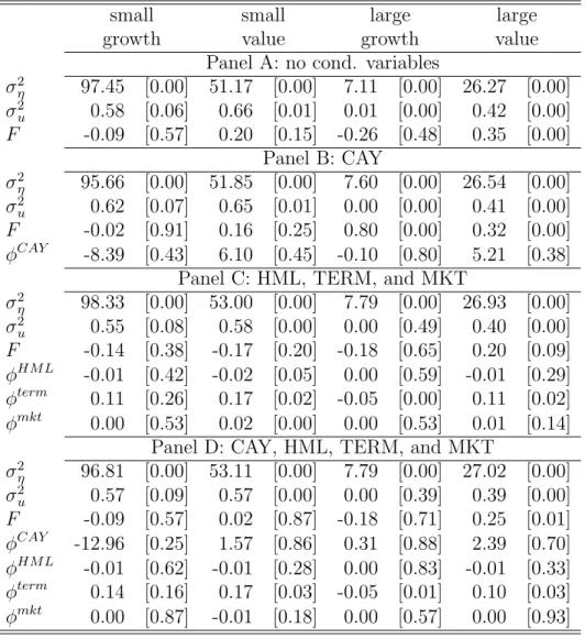
The parameter estimates of the system (5) are reported in Table 1. We estimate four specifications of the learning model. In the first specification in Table 1, no conditioning variables are included. We then present estimates where CAY is the only conditioning variable: this specification is a learning augmented version of Lettau and Ludvigson (2001). The third model uses the conditioning variables from Campbell and Vuolteenaho (2004): the term spread, the market return, and the value spread (HML). In the last specification, we include all four conditioning variables in the estimation. In order to keep Table 1 readable, we only report the parameter estimates for four portfolios: small-growth, small-value, large-growth, and large-value.
Estimates of the idiosyncratic return variance ¡σi η
¢2
and the idiosyncratic beta variance (σi
u)
2 vary little across different specifications (reading Table 1 vertically), but do vary
sub-stantially across different portfolios (reading Table 1 horizontally). The idiosyncratic return variance ¡σi
η
¢2
is highest for the small growth and lowest for the large growth portfolio. Small stocks and growth stocks have higher variance of idiosyncratic shocks to betas (σi
u)
2
(except in the last specification). The coefficient of auto-regression Fi does vary substan-tially across different model specifications, suggesting that conditioning variables pick up some of the persistence in betas. Value stocks are positively autocorrelated with estimates of Fi between 20% and 35% in the model without conditioning variables, whereas growth
stocks have a (small) negative autocorrelation around the long-run mean Bi. Deviations of value stocks from the long-run mean Bi are thus more persistent.
For the four portfolios that we report in Table 1, only the term spread is a conditioning variable that is consistently significant, whereas CAY, the market, and HML never appear to be significant. Each of the conditioning variables, however, is significant for at least one of the portfolios that we do not report here. Furthermore, we show in the next section that pricing errors are changing substantially with different conditioning variables, meaning that these instruments are relevant conditioning information. Betas of the large growth portfolio depend negatively on the term premium, whereas the betas of the other portfolios depend positively on the term premium. The term spread predicts recessions: in the postwar period, every time the term spread became negative, a recession followed (see Estrella and Hardouvelis (1991) and Stock and Watson (1989)). This finding suggests that expected returns of large growth stocks increase relative to other portfolios when the market expects a recession. The betas of growth stocks load negatively on CAY, whereas value stocks load positively on CAY. Lettau and Ludvigson (2001) argue that CAY is high during recessions and low in expansions, suggesting that the value premium is partially explained by the increase in betas during recessions. In our context, loadings of betas on HML and the market are small in magnitude and insignificant, which makes them hard to interpret.
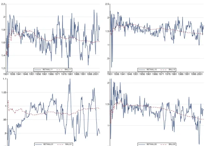
Let us now turn directly to the filtered series of the factor loadings. Figure 1 plots the step-ahead forecast level bie
t+1|t and forecast long-run mean Btie+1|t series resulting from the Kalman filter for the four portfolios of Table 1. The graphs show a pattern that has been pointed out in Franzoni (2002): starting from the late forties, there was a downward trend in the betas of value and small stocks (see portfolios 1:1, 1:5, and 5:1). The flip side of the coin is that the beta of large growth stocks displays an upward trend. However, relative to the rolling-window OLS estimates of Franzoni, our Kalman filter betas vary more slowly. This fact is due to the Bayesian updating contained in the Kalman filter and to the assumption of mean-reversion, which cause some positive weight to be attached to past levels of beta. The graphs also show how the forecast level of beta is anchored to the forecast level of the
long-run mean, which in turn evolves in a smooth fashion.
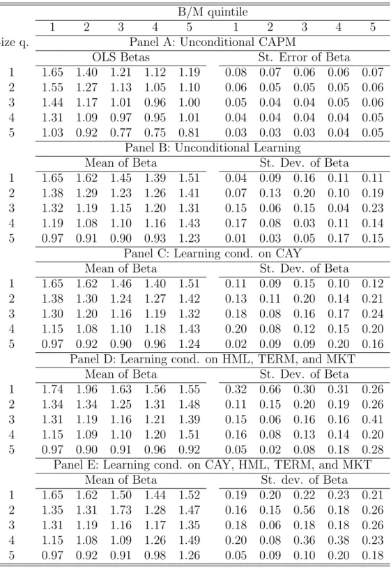
Table 2 provides evidence on the relationship between OLS beta estimates and Kalman filtered betas. Panel A contains the OLS beta estimates from time-series regressions in the sample between 1963:Q3 and 2004:Q4, while Panels B and C have summary statistics on the
bie
t+1|t series in the same period. The crucial point to notice is that, when there is evidence of a descending trend in beta, as for value and small portfolios, the two filtered beta series tend to lie above the OLS estimates. This occurs because the mean-reversion assumption embedded into the filter causes the current estimate of beta to be affected by the high levels of the loading from the past. Consider, for example, portfolio 1:5 (small-value): the OLS estimate of beta is 1.19, while the Kalman filtered level of beta across models has a mean value that is always above 1.50. The opposite happens for large-growth portfolios, although to a smaller extent.
The wedge introduced by learning and mean-reversion between Kalman filtered betas and OLS estimates is at the core of our account of the mispricing, which is commonly detected in the context OLS time-series regressions. The fact that the Kalman filtered beta is higher than the OLS estimate for value portfolios is crucial to explain a fraction of the value premium as the expected return required by investors, who are learning about the true level of beta.
Finally, we need to point out that for the wedge between Kalman filtered betas and OLS estimates to exist, it is important that we let the Kalman filter start at the beginning of the longer sample. It is in the years up to the early sixties that the betas of value and small stocks had the very large realizations, which affected the forecast of the long-run mean thereafter. Accordingly, the assumption of mean reversion is also crucial to obtain a wedge. We have estimated a separate model in which we allow for non-stationarity in beta. In this case, the anchoring effect of the long-run mean disappears, and the filtered beta is very close to the betas that can be obtained from rolling window OLS estimation.7
3. Pricing Errors of the Learning-CAPM
In this section, we use the learning-augmented version of CAPM to explain average returns on a set of test assets. As said above, the analysis focuses on the twenty-five size and B/M sorted portfolios of Fama and French (1993), which have proved to be mostly problematic for CAPM.
The returns to be explained span the interval between the third quarter of 1963 and the last quarter of 2004. There are two reasons to give more attention to this later period. First, the major failures of CAPM, the ‘value premium’ and the ‘small firm effect’, are detected in these data. As we wish to investigate to what extent learning about betas can account for these anomalies, it is this sample that is of interest to us. Second, the key element in our approach is the wedge between true riskiness, which is not observed, and expected riskiness, which determines the premium required by investors. This wedge is the larger, the bigger the changes in the underlying factor loadings have been in the past. So, the wedge is more likely to be a significant determinant of expected returns in the second sub-sample, as the more drastic changes in the beta of value and small stocks occurred in the initial forty years of data.
Lewellen and Nagel (2005) suggest that the good performance of conditional asset pricing models may result from the cross-sectional design adopted for the test of these models and the failure to impose the theoretical constraints in the estimation process. They argue that time-series tests are, therefore, more suitable to these models. Accordingly, we choose to assess the performance of the learning-augmented version of CAPM in a time-series framework.
The fact that betas are estimated with a Kalman filter raises two methodological issues, which are not present in standard time-series tests of CAPM.
First, portfolio mispricing cannot be computed as the intercept in a time-series OLS regression. Hence, we proceed as follows. Each month we estimate a realization of the mispricing of portfolio i as ˆ αit+1 =Ri t+1−βˆ i kf t+1|tRtm+1, (6)
where ˆβi kft+1|t is the one-period ahead forecast of beta made at time t, which results from the Kalman filter. Then, the final estimate of the pricing error for portfolio i, ˆαi, equals the time-series mean of ˆαit+1. Analogously to the Fama and MacBeth (1973) approach, the standard error for this estimate of mispricing is computed as the standard error of the mean. The second issue has to do with the fact that the tests for the joint significance of the pricing errors, such as the Gibbons, Ross, and Shanken (1989) small sample test and the asymptotic chi-squared tests (see Cochrane (2001)), cannot be applied to our estimates of pricing errors, because the above mentioned results are valid in case of OLS estimates. Therefore, we provide bootstrapped p-values of two summary statistics of aggregate pricing error. The first summary measure is simply the square root of the mean squared pricing errors (RMSE). While this statistic gives equal weight to each pricing error, it has the appealing feature of corresponding to the objective function that is minimized in a least square problem and it has, therefore, an intuitive interpretation (see Cochrane (1996)). Following Campbell and Vuolteenaho (2004), our second statistic is the composite pricing error (CPE), which is defined as ˆα0Ωˆ−1αˆ, where ˆα is an N-dimensional vector of the portfolio pricing errors ˆα
i and ˆΩ is a diagonal matrix with estimated return variances on the main diagonal. This measure of aggregate pricing error gives less weight to the alphas of more volatile portfolios. The authors suggest that this statistic is better behaved than the Hansen and Jagannathan (1997) distance measure, in which a freely estimated variance-covariance matrix of returns is replaced for ˆΩ, because the high number of test assets magnifies the estimation error in the inverse matrix. The bootstrapping procedure of these statistics adjusts returns to be consistent with the pricing model before random samples are generated. Furthermore, the bootstrapped distribution is conditioned on the Kalman filtered beta series. Accounting for estimation error in betas would increase the variance of the statistic. Given that our asset pricing tests fail to reject the null hypothesis of zero pricing errors, a more dispersed distribution would only confirm this conclusion. Finally, the choice of the identity matrix and the diagonal matrix ˆΩ as weighting matrices in the quadratic forms of the two summary statistics allows comparisons of the performance among different asset pricing models. This
would not have been possible, if we had used the variance-covariance of pricing errors, which is affected by the choice of the asset pricing model.
We consider four specifications of the learning-augmented version of CAPM. The first specification does not include any conditional variable in the information set for the esti-mation of beta besides the history of realized returns. The performance of this model is assessed against that of the corresponding CAPM formulation without learning, that is the unconditional CAPM. The other three models specify three alternative sets of conditioning variables in the state equation that defines the evolution of beta (the yt variables in Equa-tion (3)). These models are contrasted to the corresponding condiEqua-tional CAPM specificaEqua-tion without learning on beta. The choice of state variables reflects the results in the literature on conditional models and is discussed in the previuos section.
Although we consider learning about unobservable factor loadings as the appropriate complement to conditional models, we want to start our analysis from two models that do not include conditioning variables in order to assess the sole contribution of learning in reducing the pricing errors. Table 3 compares the pricing errors generated by the unconditional CAPM (Panel A) with those from the learning CAPM with no conditioning variables (Panel B). In Panel A, the pricing errors are simply the intercept from time-series regressions and their
t-statistics are computed accordingly. The computation of the pricing errors and t-statistics for the learning model in Panel B reflects the procedure described above. At the bottom of the table, we provide the two summary measures of the aggregate mispricing (RMSE and CPE) along with their bootstrapped p-values.8 Panel A of Table 3 confirms known results
in asset pricing. Value stocks display positive and significant mispricing, which in the case of the small-value portfolio is about 8% annually. On the other hand, growth stocks have a discount in returns, which is marginally significant for the small-growth portfolio.
In moving from Panel A to Panel B, the general impression is that pricing errors decrease. In particular, accounting for learning reduces the alpha of the small-value portfolio by about 25% from 2.05% to 1.63% quarterly. The reduction in the mispricing of the other value portfolios is even larger and the alpha of the large-value portfolio decreases to about zero.
Also on the growth side of the spectrum, the alphas are generally reduced by the learning model, except for the small-growth portfolio. The lack of a decrease in the absolute mispric-ing of this group of stocks originates from the fact that while this portfolio has a discount in returns, its beta displays a decreasing trend (see Figure 1). Hence, there is no wedge between the OLS and the Kalman filter estimates of beta. The small-growth portfolio has proven to be problematic in the context of other studies based on these test assets (Fama and French (1993), Campbell and Vuolteenaho (2004)), suggesting that the small size of these stocks and, probably, their low liquidity, impose a separate account of their returns.
The general reduction in pricing errors achieved by the learning model in Table 3 is confirmed by looking at the two aggregate measures. In moving from the unconditional CAPM to the learning CAPM, the RMSE decreases by about 25%, whereas the CPE drops by about 45%. Most importantly, the bootstrapped p-values for these two statistics indicate that, in the case of the learning model, they are only marginally significant.
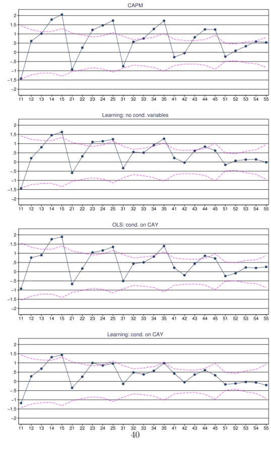
The first two graphs in Figure 2 give a visual impression of the reduction in pricing errors achieved by the learning model relative to the unconditional CAPM. Moreover, the standard error bands provide direct evidence of the fact that the variance of the estimates does not increase from one model to the other, suggesting that the larger p-values for the summary measures of mispricing in Panel B are not the result of increased sampling error.
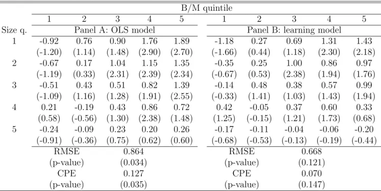
Among the conditional asset pricing models, the one by Lettau and Ludvigson (2001) has recently received much attention due to its success in substantially improving the pricing performance of the CAPM and the Consumption CAPM. As mentioned above, Lewellen and Nagel (2005) argue that the correct framework for testing this model is a time-series one. Accordingly, Panel A of Table 4 presents the time-series tests of a conditional asset pricing model, in which beta is assumed to be a linear function of Lettau and Ludvigson’s CAY. This approach is equivalent to a time-series regression of portfolio returns on two factors: the market and the market scaled by lagged CAY. Without going into the details, it is evident that, although the model decreases mispricing relative to the unconditional CAPM, the improvement is not substantial, consistent with Lewellen and Nagel’s (2005) prediction.
For example, the RMSE is reduced by just 20%.
The point of this paper is to show that the combination of conditioning variables and learning about time-varying factor loadings achieves a significant reduction in pricing errors. This argument finds a large part of its support from Panel B of Table 4, which presents the alphas from the learning model computed using CAY as conditioning variable. The comparison with Panel A of the same table suggests that learning improves the pricing performance of conditional models. All pricing erros, except for the small-growth portfolio, are smaller in Panel B. This impression is confirmed by the fact that the RMSE is reduced by about 23% and the CPE drops by about 45%. Also important, these two statistics are no longer significantly different from zero. Even more striking, there is a substantial improvement in the pricing performance with respect to both models in Table 3, which do not use conditioning variables. As an example, the decrease in the CPE relative to the unconditional CAPM is a remarkable 75%.
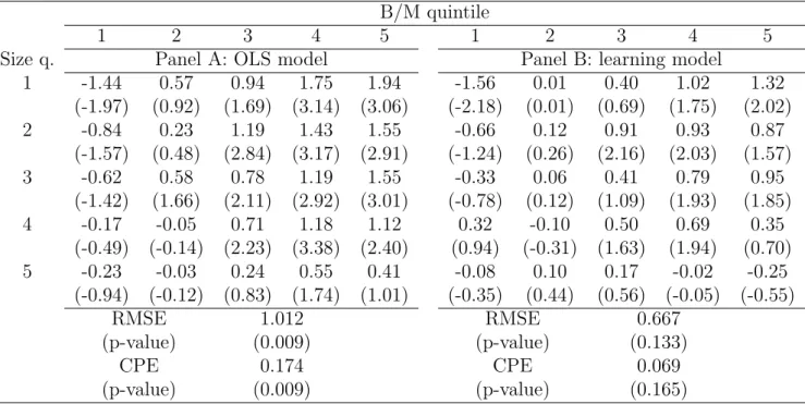
As discussed in Section 2, the conditioning asset pricing literature has proposed other conditioning variables to instrument betas besides CAY. We would like to show that the reduction in mispricing achieved by combining learning with conditional information is not specific to the choice of CAY. Among the ‘usual suspects’, and excluding CAY, we have se-lected the excess return on the market, the return on HML, and the term spread. Interacting the lags of these variables with the market return generates three additional factors in the OLS tests of CAPM. Panel A of Table 5 reports the alphas from this version of conditional CAPM. Overall, the evidence suggests that these variables are not by themselves effective in reducing CAPM pricing errors. Indeed, the RMSE and CPE are only slightly smaller than the ones in Panel A of Table 3. However, when these variables are used as instruments for beta in the Kalman filter, the performance of the resulting learning CAPM significantly improves relative to the models in Table 3 (see Panel B of Table 5). With respect to Panel A of that table, the RMSE is reduced by about 31% and the CPE by about 59%. Also with respect to Panel B of Table 3 the reduction is sensible. Therefore, we infer that the ability of learning to reduce pricing errors is not peculiar to the use of CAY as conditioning variable.
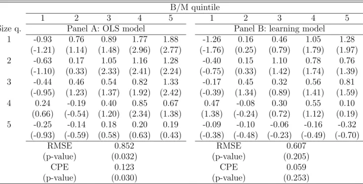
The evidence in the previous tables suggests that combining CAY with the three other conditioning variables should further improve the performance of the learning CAPM. This specification is considered in Table 6. Panel A of the table reports the pricing errors for the OLS conditional model. The results indicate that this conditional version of CAPM does not reduce pricing errors more than the specification with CAY alone. The p-values for the statistics RMSE and CPE state the rejection of this asset pricing model.
Instead, Panel B of Table 6, where the four conditioning variables are incorporated into the Kalman filter for beta, tells a completely different story. In general, the pricing errors are smaller in absolute value than in Panel A, the main exception being again the small-growth portfolio. In particular, the premium to the value portfolios is substantially smaller than with the previous models (see also Figure 2). The alpha of the small-value portfolio is only marginally statistically significant and it drops to about 5% in annual terms. The decrease in the aggregate pricing error relative to the unconditional CAPM and the conditional models without learning is substantial. For example, the RMSE and CPE are respectively 56% and 30% of the corresponding levels for the unconditional CAPM in Table 3. Finally, these two statistics are not significantly different from zero, suggesting that the asset pricing model is not rejected by the data. As said before, given that the standard error of the alphas for this model and the bootstrapped standard deviation of these two statistics are not significantly larger than for the unconditional CAPM, which is instead rejected, we are not inclined to impute the failure to reject to the lack of statistical power with respect to the tests of the other CAPM specifications.9
Finally, it is interesting to compare the performance of our theoretically motivated learn-ing model to that of Fama and French’s (1993) empirical model, which is known to perform well on this set of test assets. Table 7 contains the alphas from the three-factor model. The Fama-French model produces smaller pricing errors for value stocks than our learning specification in Panel B of Table 6. It does, however, worse in pricing growth portfolios. In terms of aggregate mispricing, the Fama-French specification yields a RMSE which is only 19% smaller than the learning model of Table 6. The difference in the CPE is however larger,
because the three-factor model reduces the alphas of value portfolios, which have compara-tively lower return volatility and, therefore, receive more weight. Incidentally, the rejection of the Fama-French model in spite of the smallest aggregate mispricing is to be imputed to the fact that the three factors absorb most of the residual variance and, therefore, increase the power of the tests.
In conclusion, the evidence suggests that incorporating learning into conditional models pushes the pricing performance of CAPM substantially closer to that of the best multi-factor models.
4. Related Literature
In terms of modelling strategy, our work has drawn inspiration from Lewellen and Shanken (2002). These authors extend results by Timmermann (1993) to an equilibrium setting with multiple securities. Lewellen and Shanken show that learning about the unobservable means of the dividends generates both predictability and excess variance in returns. More generally, their goal is to point out the role played by parameter uncertainty in explaining pricing anomalies. While placing our paper in this line of research, we innovate by focusing on uncertainty about second moments. The advantage of this choice is to capture the impact of the long-run behavior of risk for today’s expected returns. This element is missed if one focuses only on the long-run mean of the dividend process.
Our learning story is related to Sargent (2002). Sargent attributes the rise and fall of inflation in the post-war period to a learning problem. Policy makers had a particular prior about the structural relationship between inflation and unemployment. Sargent argues that policy makers inferred the true relationship between inflation and unemployment only over time. Similarly, in our approach, investors learn slowly the true riskiness of portfolios, as they need a long time-series of data to infer the long-run mean of beta. From our point of view, modeling the evolution of expectations of risk premia explicitly is an appealing economic story.
Previous literature has modeled unobservable factor loadings by studying portfolio choice in a Bayesian setting (e.g., Pastor (2000), Pastor and Stambaugh (2000)). These papers, however, adopt a partial equilibrium approach and are not concerned with the implications for equilibrium expected returns, which is the focus of this work.
Rationality implies that conditional expectations evolve according to Bayes’ rule, which naturally leads to modeling the evolution of investor’s expectations via the Kalman Filter. Multivariate GARCH models are an econometric alternative to Kalman filtered estimates of beta. For example, Engle, Bollerslev, and Wooldridge (1988) and Engle, Lilien and Robins (1987) test a CAPM models where the time-variation in beta is modeled as a (multivariate) GARCH. Engle and Lee (1999) adopt a model of volatility that is closely related to ours. They model the volatility of the market return as an autoregressive process that is reverting back to a slowly time-varying mean. Instead of modeling the time-variation of volatilities, we model the time-variation of betas. Schwert and Seguin (1990) also model the time-variation of covariances in a Garch framework and test the CAPM with time-varying betas on the universe of size-sorted portfolios. The main econometric difference to our approach is that our analysis allows idiosyncratic movements in beta.
When second moments are constant, their estimation can be arbitrarily improved by increasing the frequency of observations (Merton (1980)). When second moments are time-varying, increasing the frequency of observations can lead to improved efficiency even when the wrong structural model of second moments is imposed (Nelson (1992) and Diebold, Andersen, Bollerslev, and Labys (2003)). The driving forces for our results is the evolution of the long-run mean of betas. An increase in the frequency of the data does not help to make better inference about the long-run mean of beta, only a longer time-series can improve investors’ inference about the long-run mean.
5. Conclusions
In deriving factor pricing models, the existing literature has proceeded in one of two ways: either by assuming that second moments and risk premia are constant to derive unconditional restrictions, or by modelling the evolution of conditional moments as constant functions of state variables. We extend the latter approach by introducing unobserved, idiosyncratic movements in beta. Given the normality assumption, it follows naturally from Bayes’ rule to model investors’ learning about beta via the Kalman Filter.
We perform time-series asset pricing tests on the size and B/M sorted portfolios. The introduction of learning into standard conditional CAPM models, by estimating betas with the Kalman filter, reduces pricing errors substantially. Whereas standard conditional CAPM formulations are rejected in the time-series, our learning augmented specifications cannot be rejected.
We have made some simplifying assumptions that could be relaxed in future research. Throughout the paper, we have assumed that betas evolve as linear, autoregressive processes with homoskedastic innovations. Nonlinear Bayesian estimation methods such as Monte-Carlo Markov-Chains would allow the assumption of linearity and constant variances of innovations to betas to be relaxed. We have also simplified our approach by assuming that the market return is the only priced factor. It is straightforward to extend our methodology to a setting with multiple factors. One of the appealing features of our approach, however, is to show that a one-factor model can go a long way in explaining stock returns, once learning about systematic risk is introduced.
Appendix 1: Derivation of the Learning-CAPM
In this appendix, we present a framework that derives equation (1) from the basic principles of no-arbitrage. We denote relative excess returns to asset i by Ri
t+1. Ross (1976b) shows
- in what has become to be known as the fundamental theorem of asset pricing - that the absence of arbitrage implies the existence of a strictly positive pricing kernelMt+1 such that
Et
£
Mt+1Rit+1
¤
= 0 (7)
Most asset pricing models can be derived from Equation (7) with an appropriate specification of the stochastic discount factor. We assume that unexpected returns depend linearly on surprises to the stochastic discount factor:
Ri t+1−Et £ Ri t+1 ¤ =−bi t+1(Mt+1−Et[Mt+1]) +εit+1 (8) where εi
t+1 denotes idiosyncratic risk, which is a random variable that is independently
distributed of Mt+1, while bit+1 is the loading of asset returns on the pricing kernel. The
assumption that return surprises depend linearly on innovations to the discount factor is standard. It holds naturally in continuous time, and is also assumed in the derivation of the APT. An implicit assumption in (8) is that innovations to the pricing kernel depend on only one source of risk. We make this assumption as we focus on pricing models with a single risk factor in our empirical application. However, we could have assumed that shocks to Mt+1
are subject to shocks from multiple sources, everything that follows could easily be extended to such a setting.
We denote the value weighted excess return of the market portfolio by RM
t+1 and assume
that the idiosyncratic risk in factor loadings bi
t+1 averages out cross-sectionally. The value
weighted cross-sectional average of factor loadingsbi
t+1 is thus known at timetand we denote
it by ¯bt. We further assume that the value weighted idiosyncratic risk averages to zero. The value weighted average of Equation (8) then implies the following unexpected return to the
market portfolio:
RMt+1−Et
£
RtM+1¤=−¯bt(Mt+1−Et[Mt+1]) (9)
Surprises in the market return thus depend linearly on surprises in the pricing kernel. We have not restricted the sign of ¯bt, but we would expect it to be positive in normal times: a surprisingly high realization of the stochastic discount factor leads to stronger discounting and thus lower returns.
Replacing Equations (8) and (9) into Equation (7) and combining gives the following expression for excess returns to individual assets:
Rit+1 =βit+1RMt+1+¡βiet+1|t−βit+1¢Et
£
RMt+1¤+εit+1 (10) where the beta of asseti is defined asβi
t+1 =bit+1/¯bt and βiet+1|t=Et £ βi t+1|Mt+1 ¤ . Note that Et £ βit+1|Mt+1 ¤ = Et £ βit+1|RM t+1 ¤
: the market return is a sufficient statistic for the pricing kernel. Individual returns are determined by three components. The first component is the market return RM
t+1 times the systematic risk βit+1: assets with a higher beta have more
systematic risk, and investors are compensated for that risk with higher returns. The second term is the surprise in factor loadings: a positive shock to the factor loading of assetibetween
t and t+ 1 requires expected returns to increase and hence prices to fall, which explains the negative dependence ofRi
t+1 onβit+1−βiet+1|tsurprises to asset betas. The third determinant of returns is the idiosyncratic return εi
t+1. By taking the expectation of Equation (10), we
can see that the conditional CAPM holds:
Et £ Ri t+1 ¤ =βiet+1|tEt £ RM t+1 ¤ (11) Furthermore, covt ¡ Ri t+1, RMt+1 ¢ /vart ¡ RM t+1 ¢ =βie t+1|t. Finally, by denoting ηi t+1 = ¡ βiet+1|t−βit+1¢Et £ RM t+1 ¤ +εi t+1 (12) we obtain equation 1.
Appendix 2: Derivation of the Kalman-Filter
This section gives the details about the Kalman filter. Let’s introduce the following notation:
ξi t= Bi βit F˜i = 1 0 1−Fi Fi Ht = 0 RM t Ui t+1 = 0 ui t+1 Φi0 t = 0 φi0yt
Then the system of Equations (5) can be written as:
ξit+1 = F ξ˜ it+ Φi0Yt+Uti+1 ∀i (13)
Rit = Ht0ξit+ηit ∀i (14)
Furthermore denote the variance-covariance matrix of the forecast error as follows: Γi t+1|t=E h¡ ξi t+1−E £ ξi t+1|=t ¤¢ ¡ ξi t+1−E £ ξi t+1|=t ¤¢0 |=t i (15) With this notation, the Kalman-Filter from Hamilton (1994) can be directly applied:
E£ξi t+1|=t ¤ = F˜iE£ξi t|=t−1 ¤ +κi t ¡ Ri t−Ht0E £ ξi t|=t−1 ¤¢ (16) κi t = F˜iΓit|t−1Ht ¡ H0 tΓit|t−1Ht+σiη2 ¢−1 (17) Now, using the notation introduced in Section 1 we obtain:
Btie βiet+1|t = Et[Bi] Et £ βit+1¤ (18) = 1 0 1−Fi Fi Btie−1 βiet|t−1 + 0 φi0yt−1 +κi t ¡ Ri t−Et−1 £ Ri t ¤¢
where κit = 1 0 1−Fi Fi Γi t|t−1 0 RM t 0 RM t 0 Γit|t−1 0 RM t +σi2 η −1 (19)
Writing each updating equation separately yields Equations (3) and (4) where:
Ki t = γit(1|t−,2)1 γit(2|t−,2)1(RM t ) 2 +σi2 η RM t kti = (1−Fi)γi(1,2) t|t−1+γ i(2,2) t|t−1Fi γit(2|t−,2)1(RM t ) 2 +σi2 η RM t κit= ³ Ki t kti ´0 (20)
and γti(|tq,r−1) are the (q-th, r-th) element of the matrix Γi
t|t−1 which evolves as:
Γi t+1|t= ³ ˜ Fi−κi tHti ´ Γi t|t−1 ³ ˜ Fi0−Hi tκit0 ´ +σ2 ηκitκit0+ 0 0 0 σ2 u (21)
References
Andersen, T., T. Bollerslev, F. Diebold, and J. Wu, 2005, “A Framework for Exploring the Macroeconomic Determinants of Systematic Risk,” American Economic Review, forth-coming.
Ang, A., and J. Chen, 2004, “CAPM Over the Long-Run: 1926-2001,” unpublished manuscript, Columbia University and University of Southern California.
Barberis, N., and A. Shleifer, 2003, “Style Investing,” Journal of Financial Economics, 68, 161-199.
Bollerslev, T., R. Engle, and J. Wooldridge, 1988, “A capital asset pricing model with time varying covariances,” Journal of Political Economy, 96, 116-131.
Breeden, D., 1979, “An Intertemporal Asset Pricing Model with Stochastic Consumption and Investment Opportunities,” Journal of Financial Economics, 7, 265-296.
Campbell, J., 1996, “Understanding Risk and Return,” Journal of Political Economy, 104, 298-345.
Campbell, J., and T. Vuolteenaho, 2004, “Bad Beta, Good Beta,” American Economic Review, 94, 1249-75.
Chan, Y., and N. Chen, 1991, “Structural and return characteristics of small and large firms,” Journal of Finance, 46, 1467-1484.
Chen, N., R. Roll, and S. Ross, 1986, “Economic Forces and the Stock Market,” Journal of Business, 59, 383-403.
Cochrane, J., 1996, “A Cross-Sectional Test of an Investment-Based Asset Pricing Model,”
Journal of Political Economy, 104, 572-621.
Cochrane, J., 2001,Asset Pricing, Princeton University Press, Princeton, NJ.
Davis, J., E. Fama, and K. French, 2000, “Characteristics, Covariances, and Average Re-turns: 1929-1997,” Journal of Finance, 55, 389-406.
Debreu, G., 1959, Theory of Value, John Wiley and Sons, New York.
Diebold, F., T. Andersen, T. Bollerslev, and P. Labys, 2003, “Modeling and Forecasting Realized Volatility,” Econometrica, 71, 579-626.
Engle, R., T. Bollerslev and J. Wooldridge, 1988, “A Capital Asset Pricing Model with Time Varying Covariances,” Journal of Political Economy, 96, 116-131.
Engle, R., D. Lilien, and R. Robins, 1987, “Estimation of Time Varying Risk Premia in the Term Structure: the ARCH-M Model,” Econometrica, 55, 391-407.
Engle, R., and G. Lee, 1999, “A Permanent and Transitory Component Model of Stock Return Volatility,” in: R. Engle and H. White (ed.), Cointegration, Causality, and Fore-casting: A Festschrift in Honor of Clive W.J. Granger, Oxford: Oxford University Press, 475-497.
Estrella, A. and G. Hardouvelis, 1991, “The Term Structure as a Predictor of Real Economic Activity,” Journal of Finance, 46, 555-76.
Fama, E. and J. MacBeth, 1973, “Risk, Return, and Equilibrium: Empirical Tests,” Journal of Political Economy, 81, 607-636.
Fama, E., and K. French, 1992, “The Cross-section of Expected Stock Returns,” Journal of Finance, 47, 427-465.
Fama, E., and K. French, 1993, “Common Risk Factors in the Returns on Stocks and Bonds,”
Journal of Financial Economics, 33, 3-56.
Ferson, W., and C. Harvey, 1999, “Conditioning variables and the cross-section of stock returns,” Journal of Finance, 54, 1325-1360.
Ferson, W., S. Kandel, and R. Stambaugh, 1987, “ Tests of Asset Pricing with Time-Varying Expected Risk Premiums and Market Betas,” Journal of Finance, 42, 201-220.
Franzoni, F., 2002, “Where is beta going? The Riskiness of Value and Small Stocks,” Ph.d. dissertation, MIT.
Gibbons, M., S. A. Ross, and J. Shanken, 1989, “A Test of the Efficiency of a Given Port-folio,” Econometrica, 57, 1121-52.
Hamilton, J. D., 1994, Time Series Analysis. Princeton, NJ: Princeton University Press. Hansen, L., R. Jagannathan, 1997, “Assessing Specification Errors in Stochastic Discount
Factor Models,” Econometrica, 55, 587-614.
Harvey, C., 1989, “Time-Varying Conditional Covariances in Tests of Asset Pricing Models,”
Journal of Financial Economics, 24, 289-317.
Jagannathan, R., and Z. Wang, 1996, “The Conditional CAPM and the Cross-Section of Expected Returns,” Journal of Finance, 51, 3-53.
Jegadeesh, N., and S. Titman, 1993, “Returns to Buying Winners and Selling Losers: Im-plications for Stock Market Efficiency,” Journal of Finance, 48, 65-91.
Jostova, G., and A. Philipov, 2004, “Bayesian Analysis of Stochastic Betas,” Journal of
Financial and Quantitative Analysis, forthcoming.
Koopman S. J., and J. Durbin, 2001, Time Series Analysis by State Space Methods, Oxford University Press.
Lettau, M., and S. Ludvigson, 2001, “ Resurrecting the (C)CAPM: A Cross-Sectional Test When Risk Premia Are Time-Varying,” Journal of Political Economy 109, 1238-1287. Lewellen, J., and S. Nagel, 2005, “The Conditional CAPM Does Not Explain Asset-Pricing
Anomalies,” Journal of Financial Economics, forthcoming.
Lewellen, J., and J. Shanken, 2002, “Learning, Asset-pricing Tests, and Market Efficiency,”
Journal of Finance 57, 1113-1145.
Lucas, R., 1978, “Asset Prices in an Exchange Economy,” Econometrica, 46, 1429-1446. Lustig, H., and S. Van Nieuwerburgh, 2005, “Housing Collateral, Consumption Insurance
and Risk Premia: an Empirical Perspective,” Journal of Finance, forthcoming.
Merton, R. C., 1980, “On Estimating the Expected Return on the Market: an Exploratory Investigation,” Journal of Financial Economics, 8, 323-361.
Nelson, Daniel B., 1992, “Filtering and Forecasting with Misspecified ARCH Models I: Get-ting the Right Variance with the Wrong Model,” Journal of Econometrics, 52, 61-90. Pastor, L., 2000, “Portfolio Selection and Asset Pricing Models,” Journal of Finance, 55,
179-223.
Pastor, L., and Stambaugh, R., 2000, “Comparing Asset Pricing Models: An Investment Perspective,” Journal of Financial Economics 56, 335-381.
Ross, S., 1976a, “The Arbitrage Theory of Capital Asset Pricing,” Journal of Economic Theory, 13, 341-360.
Ross, S., 1976b, “Risk, Return, and Arbitrage,” in I. Friend and J. Bicksler (eds.),Risk and
Return in Finance, Volume 1, Ballinger, Cambridge, 189-218.
Santos, T., and P. Veronesi, 2004, “Conditional Betas,” unpublished manuscript, Columbia University and University of Chicago.
Sargent, T., 2002, The Conquest of American Inflation, Princeton: Princeton Univerity Press.
Schwert, G. W., and P. Seguin, 1990, “Heteroskedasticity in Stock Returns,” Journal of Finance, 45, 1129-1155.
Shanken, J., 1990, “Intertemporal Asset Pricing: An Empirical Investigation,” Journal of Econometrics, 45, 99-120.
Stock, J., and M. Watson, 1989, “New Indexes of Coincident and Leading Economic In-dicators,” in: NBER Macroeconomic Annuals 1989, O. Blanchard and S. Fisher (eds.), Cambridge, MA: MIT Press.
Timmermann, A., 1993, “How Learning in Financial Markets Generates Excess Volatility and Predictability in Stock Price,” Quarterly Journal of Economics, 108, 1135-1145.
Notes
1Some of the earlier asset pricing papers that model the evolution of conditional
mo-ments are, among the others, Ferson, Kandel, and Stambaugh (1987), Bollerslev, Engle, and Wooldridge (1988), Harvey (1989). A more recent example that follows a similar approach is Ferson and Harvey (1999). Multifactor models with conditioning information include Shanken (1990) and Lustig and Van Nieuwerburgh (2005). Two papers that explore de-terminants of time-varying betas are Santos and Veronesi (2004) and Andersen, Bollerslev, Diebold and Wu (2005).
2See, for example, Barra’s Newsletter from September 1988: “What’s new about Beta?” 3We did estimate a different specification, in which B is an observable parameter rather
than a latent variable. In this case,Bis estimated using maximum likelihood in the same way as other parameters of the Kalman filter. This alternative specification, which is available upon request, gives results that produce somewhat larger pricing errors than the ones we present in the paper.
4The porfolio returns are from Prof. Ken French’s website.
5The results with monthly data can be provided by the authors upon request. 6This fact can be seen by replacing Equation (9) into Equation (7), which gives:
Et[RMt+1] = ¯btV art £ RM t+1 ¤ Rft.
That is, the expected return on the market is proportional to ¯bt, which in turn is a function of the conditioning variables.
7A simple way to allow for non-stationarity of the factor loading is to modify the second
State Eq 2 :Bi
t+1 =Bti+vti+1
and to let the variance ofvi
t+1 be different from zero. In this case, Bt follows a random walk, and the factor loading is non-stationary. The estimates obtained with this new system are available from the authors upon request.
8In the case of the OLS models, the bootstrapping procedure re-estimates beta at each
draw. The sampling error in the estimation of beta is therefore taken into account.
9For example, the bootstrapped standard deviation of the CPE statistic for the
uncondi-tional CAPM in Panel A of Table 3 is 0.034, while it is 0.038 for the learning model in Panel B of Table 6. The two standard deviations are, therefore, very close.
Table 1: Parameter Estimates. For the twenty-five size and B/M sorted portfolios, the table reports the maximum likelihood parameter estimates for the parameters in system (5). Except Panel A, each panel corresponds to a different set of state variables in the state equation of the system. The estimated parameters are the autoregression coefficientF, the variance of the error in the observable equation (σ2
η), and the variance of the error in the state equation 1 (σ2u). P-values are given in brackets. The Kalman filter is estimated on all available data between between 1926:Q3 and 2004:Q4. CAY is available between 1951:Q4 and 2003:Q2. Portfolio returns and the other state variables (HML, term, and the market return) are available on the whole sample.
small small large large
growth value growth value
Panel A: no cond. variables
σ2 η 97.45 [0.00] 51.17 [0.00] 7.11 [0.00] 26.27 [0.00] σ2 u 0.58 [0.06] 0.66 [0.01] 0.01 [0.00] 0.42 [0.00] F -0.09 [0.57] 0.20 [0.15] -0.26 [0.48] 0.35 [0.00] Panel B: CAY σ2 η 95.66 [0.00] 51.85 [0.00] 7.60 [0.00] 26.54 [0.00] σ2 u 0.62 [0.07] 0.65 [0.01] 0.00 [0.00] 0.41 [0.00] F -0.02 [0.91] 0.16 [0.25] 0.80 [0.00] 0.32 [0.00] φCAY -8.39 [0.43] 6.10 [0.45] -0.10 [0.80] 5.21 [0.38] Panel C: HML, TERM, and MKT
σ2 η 98.33 [0.00] 53.00 [0.00] 7.79 [0.00] 26.93 [0.00] σ2 u 0.55 [0.08] 0.58 [0.00] 0.00 [0.49] 0.40 [0.00] F -0.14 [0.38] -0.17 [0.20] -0.18 [0.65] 0.20 [0.09] φHM L -0.01 [0.42] -0.02 [0.05] 0.00 [0.59] -0.01 [0.29] φterm 0.11 [0.26] 0.17 [0.02] -0.05 [0.00] 0.11 [0.02] φmkt 0.00 [0.53] 0.02 [0.00] 0.00 [0.53] 0.01 [0.14] Panel D: CAY, HML, TERM, and MKT
σ2 η 96.81 [0.00] 53.11 [0.00] 7.79 [0.00] 27.02 [0.00] σ2 u 0.57 [0.09] 0.57 [0.00] 0.00 [0.39] 0.39 [0.00] F -0.09 [0.57] 0.02 [0.87] -0.18 [0.71] 0.25 [0.01] φCAY -12.96 [0.25] 1.57 [0.86] 0.31 [0.88] 2.39 [0.70] φHM L -0.01 [0.62] -0.01 [0.28] 0.00 [0.83] -0.01 [0.33] φterm 0.14 [0.16] 0.17 [0.03] -0.05 [0.01] 0.10 [0.03] φmkt 0.00 [0.87] -0.01 [0.18] 0.00 [0.57] 0.00 [0.93]
Table 2: Summary Statistics for Betas. Panel A reports the estimates of beta and their standard errors from time-series regressions of portofolio excess returns on the excess return on the value-weighted market index. The test assets are the twenty-five size and B/M sorted portfolios. For the same assets, Panel B reports the mean of the Kalman-filtered estimates of beta and their standard deviations, when no conditioning variables are included in the state equations. Panels C to E report means and standard deviations of Kalman-filtered estimates of beta, when conditioning variables are included in the state equations. The sets of conditioning variables are given in the table. Returns are quarterly compounded returns. The sample period is 1963:Q3-2004:Q4.
B/M quintile
1 2 3 4 5 1 2 3 4 5
Size q. Panel A: Unconditional CAPM
OLS Betas St. Error of Beta
1 1.65 1.40 1.21 1.12 1.19 0.08 0.07 0.06 0.06 0.07 2 1.55 1.27 1.13 1.05 1.10 0.06 0.05 0.05 0.05 0.06 3 1.44 1.17 1.01 0.96 1.00 0.05 0.04 0.04 0.05 0.06 4 1.31 1.09 0.97 0.95 1.01 0.04 0.04 0.04 0.04 0.05 5 1.03 0.92 0.77 0.75 0.81 0.03 0.03 0.03 0.04 0.05
Panel B: Unconditional Learning
Mean of Beta St. Dev. of Beta
1 1.65 1.62 1.45 1.39 1.51 0.04 0.09 0.16 0.11 0.11 2 1.38 1.29 1.23 1.26 1.41 0.07 0.13 0.20 0.10 0.19 3 1.32 1.19 1.15 1.20 1.31 0.15 0.06 0.15 0.04 0.23 4 1.19 1.08 1.10 1.16 1.43 0.17 0.08 0.03 0.11 0.14 5 0.97 0.91 0.90 0.93 1.23 0.01 0.03 0.05 0.17 0.15
Panel C: Learning cond. on CAY
Mean of Beta St. Dev. of Beta
1 1.65 1.62 1.46 1.40 1.51 0.11 0.09 0.15 0.10 0.12 2 1.38 1.30 1.24 1.27 1.42 0.13 0.11 0.20 0.14 0.21 3 1.30 1.20 1.16 1.19 1.32 0.18 0.08 0.16 0.17 0.24 4 1.15 1.08 1.10 1.18 1.43 0.20 0.08 0.12 0.15 0.20 5 0.97 0.92 0.90 0.96 1.24 0.02 0.09 0.09 0.20 0.16
Panel D: Learning cond. on HML, TERM, and MKT
Mean of Beta St. Dev. of Beta
1 1.74 1.96 1.63 1.56 1.55 0.32 0.66 0.30 0.31 0.26 2 1.34 1.34 1.25 1.31 1.48 0.11 0.15 0.20 0.19 0.26 3 1.31 1.19 1.16 1.21 1.39 0.15 0.06 0.16 0.16 0.41 4 1.15 1.09 1.10 1.20 1.51 0.16 0.08 0.13 0.14 0.20 5 0.97 0.90 0.91 0.96 0.92 0.05 0.02 0.08 0.18 0.28
Panel E: Learning cond. on CAY, HML, TERM, and MKT
Mean of Beta St. dev. of Beta
1 1.65 1.62 1.50 1.44 1.52 0.19 0.20 0.22 0.23 0.21 2 1.35 1.31 1.73 1.28 1.47 0.16 0.15 0.56 0.18 0.26 3 1.31 1.19 1.16 1.17 1.35 0.18 0.06 0.18 0.18 0.26
Table 3: Alphas: No Conditioning Variables. Panel A reports the intercept from OLS time-series regressions of portofolio excess returns on the excess return on the value-weighted market index. The test assets are the twenty-five size and B/M sorted portfolios. For the same assets, Panel B reports the alphas for the learning model without conditioning variables. For each portfolio, alpha is computed as the portfolio times series mean of the time t excess portfolio return minus the time t product of the Kalman filter estimate of beta and the excess return on the market.
t-statistics are given in parentheses below each estimate. For the learning models the standard errors are computed from the time-series standard deviation of time the t pricing error. Below each estimate,t-statistics are given in parentheses. At the bottom of each panel the table reports three statistics: the square root of the mean squared pricing error over the twenty-five portfolios (RMSE); the composite pricing error (CPE), which is a quadratic form in the vector of the twenty-five portfolio pricing errors, where the weighting matrix is a diagonal matrix with estimated return variances on the main diagonal; and the bootstrapped p-value for these two statistics. Returns are quarterly compounded returns. The sample period is 1963:Q3-2004:Q4.
B/M quintile
1 2 3 4 5 1 2 3 4 5
Size q. Panel A: OLS model Panel B: learning model
1 -1.42 0.61 1.02 1.78 2.05 -1.43 0.21 0.80 1.46 1.63 (-1.97) (0.99) (1.82) (3.17) (3.17) (-2.02) (0.33) (1.37) (2.52) (2.43) 2 -0.93 0.25 1.22 1.47 1.73 -0.59 0.31 1.09 1.13 1.24 (-1.77) (0.54) (2.92) (3.27) (3.21) (-1.12) (0.65) (2.57) (2.44) (2.18) 3 -0.76 0.57 0.75 1.27 1.71 -0.33 0.54 0.51 0.92 1.26 (-1.75) (1.66) (2.04) (3.09) (3.35) (-0.78) (1.58) (1.36) (2.14) (2.43) 4 -0.26 -0.04 0.82 1.25 1.24 0.22 -0.03 0.61 0.84 0.62 (-0.74) (-0.13) (2.56) (3.61) (2.69) (0.62) (-0.11) (1.88) (2.31) (1.21) 5 -0.23 0.08 0.33 0.59 0.54 -0.15 0.07 0.13 0.14 -0.01 (-0.95) (0.37) (1.17) (1.90) (1.34) (-0.64) (0.31) (0.44) (0.42) (-0.03) RMSE 1.076 RMSE 0.814 (p-value) (0.008) (p-value) (0.041) CPE 0.197 CPE 0.108 (p-value) (0.009) (p-value) (0.057)