Basis risk in static versus dynamic longevity-risk
hedging
∗Clemente De Rosa†, Elisa Luciano‡, Luca Regis
October 19, 2015
Abstract
This paper provides a tractable, parsimonious model for assessing basis risk in longevity and its eect on the hedging strategies of Pen-sion Funds and annuity providers. Basis risk is captured by a single parameter, that measures the co-movement between the portfolio and the reference population's longevity. The paper sets out the static, full and customized swap-hedge for an annuity, and compares it with a dynamic, partial and index-based hedge. We calibrate our model to the UK and Scottish populations. The eectiveness of static ver-sus dynamic strategies depends on the rebalancing frequency of the second, on the relative costs, and on basis risk, which does not aect fully-customized, static hedges. We show that appropriately calibrated dynamic hedging strategies can still be reasonably eective, even at low rebalancing frequencies.
Keywords: longevity risk, customized vs. indexed hedge, longevity swaps, longevity bonds, rebalancing frequency.
JEL classication: G22, G32.
∗The paper has been published in the Scandinavian Actuarial Journal, Volume 4, 2017, pp. 343-365. The Authors would like to thank conference participants to the IRMC Conference 2015, the 19th IME Conference, the Longevity 11 Conference. The Authors gratefully acknowledge nancial support by the Global Risk Institute, Canada.
†Collegio Carlo Alberto, [email protected], Via Real Collegio 30, 10024 Moncalieri, Italy, + 390116705228.
‡Corresponding Author. University of Torino, Collegio Carlo Alberto and Netspar; ESOMAS Department, Corso Unione Sovietica 218/bis, 10134, Torino, Italy; e-mail: [email protected]; phone number: + 390116705230 (5200).
IMT Institute for Advanced Studies Lucca and Collegio Carlo Alberto; AXES Re-search Unit Piazza San Francesco 19, 55100 Lucca, Italy; e-mail: [email protected].; phone number: +3905834326721.
1 Introduction
Pension funds and life insurance companies providing annuities are aected by the so-called longevity risk, which is the risk that people live longer than expected when the fund or company priced and reserved their policies. So, while increasing longevity is welcome from the social point of view, it is one of the risks that annuity providers - which we will call insurers for brevity - have to face. Being a systematic risk, it cannot be diversied away by increasing the size of portfolios. Still, insurers can hedge it, using mortality derivatives, which were rst proposed by Blake and Burrows (2001). So far, such derivatives have been most frequently traded over-the-counter (OTC) and written on the insurer's specic policyholders' population. So, they are customized to full the needs of the insurer. Alongside these deals, a market for standardized products has slowly emerged. These products leave the insurance company exposed to so-called basis risk, because they are written on a reference population that does not coincide with the insured one. In the surge of markets for longevity derivatives, the debate on the pros and cons of fully customized versus index-based products is very much open. In practice, actors seeking coverage with a fully customized OTC product build a full, static hedge, such as an s-forward or a longevity swap, while not fully customized derivatives (non-OTC for brevity) provide a partial, dynamic hedge.1 In the rst case, the hedging strategy is not adjusted over time. In
the second case, coverage calls for adjustment over time. In the absence of basis risk, dynamic strategies would converge to a full, instead of a partial or approximated coverage, if rebalancing would be continuous. With basis risk, they do not converge. In both cases, they "cost", in the sense that to make them self-nancing the insurer must fund them through a "bank account", whose nal value is the hedging cost. So, while static hedges have an initially dened and considerable cost, dynamic strategies have a cost, whose amount depends on the rebalancing technique, frequency and the actual path of the underlying insurance contracts. All in all, dynamic strategies are partial, leave the insurer exposed to basis risk, but have potentially smaller costs than static hedges.
Against this background, the aim of our paper is to propose a simple framework for evaluating the eectiveness of static versus dynamic longevity-hedging solutions, in the presence of basis risk. Our rst original contri-bution consists in providing a simple model for basis risk in longevity, by separating forecast errors that are common to the general and the insured population from idiosyncratic errors, which are proper of the latter popula-tion. Longevity risk is represented through a stochastic mortality approach, namely a mortality intensity which is itself a stochastic process. We model
1For a description of a customized and an index-based transaction involving JP Morgan as a buyer of longevity risk, see Barrieu et al. (2012).
basis risk by assuming that the intensity of the general population is imper-fectly correlated with the insured one. So, we encapsulate basis risk in a single, comovement parameter.
Once basis risk is modeled, our second important contribution consists in providing fair prices of static and dynamic hedging instruments in closed form. Our static hedge entails the use of an OTC longevity swap written on the portfolio population, thereby entailing no basis risk. We consider dynamic hedges that approximate the hedge up to the rst (Delta) or second (Delta-Gamma) or time (Theta) change in the longevity forecast error, and are based on index-related longevity bonds.
Third, we assess the relative eectiveness of static versus dynamic strate-gies in a calibrated environment, where the portfolio population is made by 65-year-old Scottish males and the reference is made by 65-year-old UK males. The dynamic strategy gives rise to two types of error or costs, that we disentangle: the error due to its approximated nature, together with discrete-time rebalancing (as in Dahl et al., 2011), and the error due to unhedgeable basis risk. Since these errors are stochastic, we measure them through their
99.5percentile of the bank account which makes the strategy self-nancing.
This percentile is the greatest cost that the index-based hedge may entail, in 99.5% of the possible cases. We determine the cost of the static hedge which split along the life of the swap as a fee equates the given percentile, and makes the two strategies cost the same. Beyond this maximum fee, the dynamic hedge dominates the static hedge.
To anticipate on our results, we show that when basis risk is null, the fee of the non-OTC strategy stays between0.01% and 0.06%. In this case,
the cost of dynamic hedges is due only to their partial nature, and to dis-crete hedging. Theta hedge does not improve much the eectiveness of a Delta-Gamma strategy. When there is basis risk and the dynamic hedge is performed using a Delta-Gamma-Theta strategy the fee ranges between
0.12% and 0.41%,depending on the rebalancing frequency, which stays
be-tween a quarter and one year. Comparing the two fees, with and without basis risk, we can measure the impact of basis risk. Even if the fees we computed are relatively low, the one when basis risk is present is around seven to twelve times the other, depending on the rebalancing frequency. It would be much bigger for more infrequent rebalancing and with other, less precise dynamic hedges. We conclude that basis risk might be relevant for annuity providers' hedges, but hedging strategies, if appropriately designed and calibrated, can still be very eective.
The paper unfolds as follows: in Section 2 we review some related lit-erature, in Section 3 we set up the model for longevity and nancial risk evaluation, in Section 4 we introduce basis risk. In Section 5 we present the liabilities to be hedged. In Sections 6 and 7 we present static and dynamic hedges. In Section 8 we implement the strategies on the UK-Scottish male population aged 65, both without and with basis risk, and compare their
eectiveness. The last Section summarizes and concludes.
2 Related Literature
The eectiveness of static hedging strategies in the presence of basis risk has been examined by Ngai and Sherris (2011). Comparing dierent cash-ow matching hedging strategies achieved using various instruments, such as q-forwards, longevity bonds or swaps, they show that static hedging is eective in reducing tail risk (expected shortfall) and that the impact of basis risk on eectiveness is limited. In Coughlan et al. (2011), the authors argue that, due to the lack of a proper framework to understand Basis Risk, there has been a widely diused misconception that index-based longevity hedging is ineective. So, they describe a framework to evaluate basis risk and to deter-mine the eectiveness of longevity hedging when standardized index-based instruments are used. In their case study, using bootstrap from historical data, they nd that, despite the presence of basis risk, if the correlation between the dynamics of the reference population underlying the hedging instrument and the liability portfolio one is high, the hedge remains very eective. The importance of considering basis risk is highlighted by Cairns et al. (2014), who, using simulated rather than bootstrapped data, show that population basis risk is the most important determinant of the hedge eec-tiveness of a static value-hedge longevity swap. Haberman et al. (2014) also point out the importance of assessing basis risk in indexed solutions, in order to understand the residual risk left, also in the light of Solvency II capital requirements. In their paper, they provide a comprehensive treatment of basis risk measurement, addressing the issues of model selection and proper calibration.
Li and Hardy (2011) compare four dierent extensions of the Lee-Carter model, suitable to model basis risk. The analysis identies the Augmented Common Factor model as most appropriate among those tested. Such model assumes, similarly to the model we propose in this paper, that the mortalities of two populations depend on a common and on a population-specic factor. Application to the hedging of a Canadian pension plan exposure to longevity risk using a portfolio ofq-forwards indexed to the US population shows that
a static longevity hedge can still be reasonably eective even when basis risk is present.
Continuous-time modeling and dynamic hedging of longevity basis risk, as in our paper, are tackled by Dahl et al. (2008) and Wong et al. (2014). The former consider two populations and model mortality improvements us-ing two mean-revertus-ing CIR processes driven by a bi-dimensional standard Brownian Motion. In this setting, the paper provides risk-minimizing strate-gies of longevity risk by dynamically trading in a survivor swap when basis risk is present. Wong et al. (2014) derive the mean-variance hedging strategy
for longevity risk using an instrument contingent on a mortality index, where the mortality intensity of the insurer's portfolio population is correlated and cointegrated to the mortality index itself. Dierently from these two papers, our work focuses on local rather than global hedging and provides a cali-brated assessment of the impact of basis risk and hedging frequency on the eectiveness of dynamic strategies.
3 Longevity and interest rate risk modeling
We model longevity risk assuming that the time to death of an individual belonging to a specic generation follows a Poisson process with stochastic intensity. We consider a standard ltered probability space (Ω,F,Q)
sat-isfying the usual assumptions and on which a ltration Ft is dened. The
measureQ is the so-called risk-neutral measure. Below, we will discuss the
relationship between this measure and the historical one.
The mortality intensity of a specic generation is described by a so-called Cox-Ingersoll and Ross (CIR) process, i.e. a Feller process of the type:
dλ(t) = (a+bλ(t))dt+σpλ(t)dW(t), (1)
with a > 0, b > 0, σ > 0, λ(0) = λ0 ∈ R++. The reason behind the
as-sumption b > 0 is that the process is expected to have no mean reversion.
The previous SDE describes the evolution (for a given generation) of the in-tensity of mortality arrival over calendar time. Because the generation ages over time, the drift simply ensures that the expected change in the intensity is ane and increasing in the intensity itself.
If the initial pointλ0 is strictly positive and the coecients satisfy the
fol-lowing condition:
a≥ σ
2
2 , (2)
then the mortality intensityλ(t)is strictly positive for everyt, almost surely.
Hence, to obtain a satisfactory calibrated model for the intensity process, we impose this condition on the parameters in the calibration procedure.
Consistently, we assume that the spot interest rate - or interest rate intensity - follows a CIR process of the type:
dr(t) = (¯a−¯br(t))dt+ ¯σpr(t)dW0(t), (3)
with ¯a > 0,¯b > 0,σ >¯ 0, r(0) = r0 ∈ R++, where the Wiener process W0
is independent of W.2 This last assumption entails independence between
longevity and interest rate risks. The negative sign preceding¯band its strict
positivity guarantee that the process for the interest-rate incorporates mean
2Let the ltrationF
reversion, which is a usual assumption in the interest-rate domain. The coef-cient¯bis called speed of mean reversion and represents the speed at which
the short rater(t) returns to its long-run value ¯a.
Similarly to the longevity case, the restriction on the parameters that, to-gether with the positivity of the initial pointr0, guarantees that the interest
rater(t) never turns negative is ¯
a≥ σ¯
2
2 . (4)
At each point in time, the conditional distributions of the mortality in-tensity and the interest rate are given, up to a scale factor, by a noncentral chi-square distribution.3
Denoting asτ the time to death, the conditional survival probability from tto T is
S(t, T) =P(τ >T |τ > t). (11)
To proceed to the pricing and hedging of insurance products, the risk-neutral dynamics of the two previous processes is needed. However, for calibration purposes, its eective or historical version may be the one stemming from the data, at least for the longevity case. In order to keep the notation simple, we assume that there is no risk premium in the longevity market or, equivalently, that equation (1) holds under both measures. Therefore, the
3In details, given two time instantsu < t, then the distribution ofλ(t)conditional on λ(u)is λ(t)≈σ 2 eb(t−u)−1 4b X 02 d (ν), (5) whereX02
d (ν)denotes the density of a noncentral chi-square random variable withddegrees
of freedom, where
d=4a
σ2, (6)
and the noncentrality parameterνis ν= 4be
b(t−u)
σ2(eb(t−u)−1)λ(u). (7)
Similarly, the distribution ofr(t)conditional onr(u)is r(t)≈σ¯ 2 1−e−¯b(t−u) 4¯b X 02 ¯ d (¯ν), (8) whereX02 ¯
d (¯ν)denotes the density of a noncentral chi-square random variable withd¯degrees
of freedom, with
¯ d=4¯a
¯
σ2, (9)
and the noncentrality parameterνis ¯
ν= 4¯be −¯b(t−u)
¯
calibration of the longevity intensity is performed by estimating its dynamics under the historical measure and, then, using it also under the risk-neutral measure. The calibration of the interest rate dynamics is, on the other hand, performed directly under the risk-neutral measure, thus incorporating the risk premium. As a consequence, the conditional survival probability (11) can be represented as an expectation under the risk neutral measure:
S(t, T) =EQ exp − Z T t λx(s)ds | Ft . (12)
Given our model choice, this expectation becomes:
S(t, T) =A(t, T)e−B(t,T)λ(t), (13)
whereA(t, T) andB(t, T)solve an appropriate system of Riccati equations,
being A(t, T) =A(t, T;a, b, σ) = 2γe 1 2(γ−b)(T−t) (γ −b) eγ(T−t)−1 + 2γ !2a σ2 , (14) B(t, T) =B(t, T;a, b, σ) = 2 e γ(T−t)−1 (γ−b) eγ(T−t)−1 + 2γ, (15)
whereγ =√b2+ 2σ2. As shown in Fung et al. (2014), the above specication
guarantees also that the limit of the survival probability, when T diverges,
is zero.
For any givent, it is possible to compute the log-derivative of the survival
probability, which is referred to as the "forward" mortality intensity for time
T, since it represents its forecast at timet. By denition4 f(t, T) =−∂lnS(t, T) ∂T =− ∂lnA(t, T) ∂T + ∂B(t, T) ∂T λ(t), (18)
Using a technique described in Jarrow and Turnbull (1994) and Luciano et al. (2012), which exploits the denition of "forward" intensity, we can write the survival as5
S(t, T) =e−X(t,T)I(t)+Y(t,T), (20)
4It is easy to show that ∂lnA(t, T) ∂T = 2a σ2 " 1 2(γ−b)− γeγ(T−t) eγ(T−t)−1 + 2γ γ−b # , (16) ∂B(t, T) ∂T = 4γ2eγ(T−t) [(γ−b) (eγ(T−t)−1) + 2γ]2. (17)
5Using the fact thatλ(t) =I(t) +f(0, t), (20) becomes S(t, T) =A(t, T)exp−B(t, T)hI(t)−∂lnA(t, T) ∂T (0,t)+λ(0) ∂B(t, T) ∂T (0,t) i . (19) Hence, we have an expression for the survival equivalent to (13).
whereI(t) = λ(t)−f(0, t) and X(t, T) and Y(t, T) are deterministic
func-tions of the parameters of the intensity process and of timet andT: X(t, T) = B(t, T), Y(t, T) = lnA(t, T)−B(t, T) −∂lnA(t, T) ∂T (0,t)+λ(0) ∂B(t, T) ∂T (0,t) .
The termI is called longevity risk factor. It is the dierence between the
actual intensity at timet and its forecast made at time 0. Expression (20)
will play a crucial role in hedging, because it encapsulates all riskiness in the
I factor, which has the intuitively nice interpretation of a forecast error.6
The discount factor or bond price for timet, under any stochastic process
for the spot rate, is
D(t, T) =E exp − Z T t r(u)du |Ft , (21)
which, in the CIR case, becomes
D(t, T) = ¯A(t, T)e−B¯(t,T)r(t),
where A¯(t, T) = A(t, T; ¯a,−¯b,σ¯) and B¯(t, T) = B(t, T; ¯a,−¯b,σ¯) and γ¯ =
p
¯
b2+ 2¯σ2. As in the longevity case, the bond value can be reformulated as
D(t, T) =e−X¯(t,T)J(t)+ ¯Y(t,T), (22) where ¯ X(t, T) = B¯(t, T), ¯ Y(t, T) = lnA¯(t, T)−B¯(t, T) −∂lnA¯(t, T) ∂T (0,t)+r(0) ∂B¯(t, T) ∂T (0,t) ,
and J is the nancial risk factor, measured by the dierence between the
short and forward rate:
J(t) =r(t)−F(0, t).
The forward rate F(t, T) represents the fair price at time t for a forward
contract on the spot rate at T. It is computed, similarly to the forward
6As we know, the forecast error in longevity has been substantial over the last decades. Approximately, expected lifetime improvement has been underestimated by 3 years over the last century (see International Monetary Fund (IMF) (2012)).
mortality intensity, as7 F(t, T) =−∂lnD(t, T) ∂T =− ∂lnA¯(t, T) ∂T + ∂B¯(t, T) ∂T r(t), (25)
So, also in the bond case, the reformulation in terms of the risk factor allows us to synthesize in a unique spread the forecast error that economic agents can make and that they may be willing to hedge.
4 Basis risk
Up to now we have examined a benchmark case, in which, for each sex and generation, there is a unique intensity process. To signal that, we could have used an index x for the process λ, and turned it into λx. In practice, this
setting could be restrictive. Indeed, we have non-OTC mortality derivatives written on a Reference population, while insurance companies face the need to hedge the longevity risk arising from their insureds, who represent the Portfolio population. In this case, basis risk arises since the two intensity processes governing the mortality of the two populations may dier. As a consequence, no perfect dynamic hedge is possible. Hence, the insurer willing to hedge her longevity risk can choose between a non-perfect dynamic hedge or a static hedge, such as a OTC longevity swap tailored to her Portfolio population, thus bearing no basis risk.
We focus on Delta-Gamma longevity risk hedging as a dynamic hedging strategy. To account for basis risk, we assume that the intensity of generation
x in the Reference population follows the SDE dλnpx (t) = (a+bλnpx (t))dt+σ
q
λnpx (t)dWx(t), (26)
where, to simplify notation, we omit the subscriptxfor the parameters. We
assume that the insurance portfolio is composed by a sub-population of the Reference population. The mortality intensity of generationx belonging to
the Portfolio population is
λppx (t) =δxλnpx (t) + (1−δx)λ 0 x(t), (27) with dλ0x(t) = (a0+b0λ0x(t))dt+σ0pλ0x(t)dWx0(t), (28) 7Here ∂lnA¯(t, T) ∂T = 2¯a ¯ σ2 " 1 2(¯γ+ ¯b)− ¯ γe¯γ(T−t) e¯γ(T−t)−1 + 2¯γ ¯ γ+¯b # , (23) ∂B¯(t, T) ∂T = 4¯γ2e¯γ(T−t) (¯γ+ ¯b) (eγ¯(T−t)−1) + 2¯γ2, (24)
whereWx andW
0
x are two independent standard Brownian Motions,a0 >0,
σ0 > 0, b0 ∈ R and 0 ≤ δx ≤ 1. The intensity of the insurer's Portfolio
population λppx is modelled as a convex combination of the Reference
popu-lation's intensityλnpx and an idiosyncratic componentλ
0
x orthogonal toλ np x .
The idiosyncratic component λ0x is specic to the Portfolio population and
cannot be hedged by trading in the longevity bonds written on the Reference population. Intuitively, the parameterδx measures the degree of dependence
between the evolution of the Portfolio population's mortality intensity and the Reference population one. Therefore, 1−δx could be interpreted as
a measure of basis risk. Indeed, the benchmark case without basis risk is obtained by assumingδx = 1. We assumeb0 ∈R, thus allowing the
idiosyn-cratic component to be either mean-reverting or not. The sign of b0 will
therefore be decided by the calibration that provides the lowest calibration error.
Straightforward application of Ito's Lemma shows that the dynamics of
λppx follow a two-factor CIR process. Indeed:
d δxλnpx (t) =dλ˜npx (t) = (α+β˜λnpx (t))dt+η q ˜ λnpx (t)dWx(t), (29) with α=δxa, β =b, η2 =δxσ2, and d (1−δx)λ 0 x (t) =dλ˜0x(t) = (α0+β0˜λ0x(t))dt+η0 q ˜ λ0x(t)dWx0(t), (30) with α0= (1−δx)a0, β0=b0, (η0)2= (1−δx)(σ0)2.
Since λnpx (t) and λppx (t) follow a1-factor and a2-factor CIR process
re-spectively, we can compute their conditional moments.
Assuming 0≤u≤t, in particular, the conditional covariance and
corre-lation betweenλnpx (t) and λppx (t) are
Covu λppx (t), λnpx (t) =δxV aru λnpx (t) , (31) Corru λppx (t), λnpx (t) =δx s V aru λnpx (t) V aru λppx (t) , (32)
where V aru λnpx (t)= aσ 2 2b2 e b(t−u)−12 +σ 2 b e b(t−u) eb(t−u)−1 λnpx (u), (33) V aru λ0x(t) = a 0 (σ0)2 2(b0)2 e b0(t−u)−12+ (σ 0 )2 b0 e b0(t−u) eb0(t−u)−1 λ0x(u), (34) V aru λppx (t) =δx2V aru λnpx (t) + (1−δx)2V aru λ0x(t) . (35)
Equations (31) and (32) further clarify the interpretation ofδx as a measure
of the degree of comovement between the intensity of the two populations. Indeed, when δx = 0 the two intensities have zero correlation, whileδx = 1
implies perfect positive correlation. δx positive ensures that λpp is strictly
positive. Corru
λppx (t), λnpx (t)
stays between 0 and 1. Though this may
seem restrictive, this assumption is justied by the intuition that when a shock hits the Reference population, increasing for example its mortality intensity, the sub-population is aected similarly, but with a dierent sen-sitivity, while divergence between the two intensities is entirely captured by the idiosyncratic risk factorλ0.
The survival probabilities of the Reference population are given by:
Snp(t, T) =Anp(t, T)e−Bnp(t,T)λnpx (t),
whereAnp(t, T)and Bnp(t, T) are dened as in (15). The survival
probabil-ities of the Portfolio population can be written as functions of the common and idiosyncratic intensities as follows:
Spp(t, T) = ˜Snp(t, T) ˜S0(t, T) (36) = ˜Anp(t, T) ˜A0(t, T)e−B˜np(t,T)δxλnpx (t)−B˜ 0 (t,T)(1−δx)λ 0 x(t), (37) withA˜np(t, T) =A(t, T;α, β, η),B˜np(t, T) = B(t, T;α, β, η) and A˜0(t, T) = A(t, T;α0, β0, η0),B˜0(t, T) = B(t, T;α0, β0, η0), where γ˜ = pβ2+ 2η2 and ˜ γ0 =p(β0)2+ 2(η0 )2.
As in the benchmark case, we use the Jarrow-Turnbull (1994) formula-tion of the survival probabilities in order to make their dependence on the longevity risk factor, dened asI(t) =λnpx −fxnp(0, t), explicit. The survival
probability of the Reference population can therefore be written as:
where Xnp(t, T) =Bnp(t, T), (38) Ynp(t, T) =lnAnp(t, T)−Bnp(t, T)fxnp(0, t), (39) =lnAnp(t, T)−Bnp(t, T) h −∂lnA np(t, T) ∂T (0,t) + (40) +λnpx (0)∂B np(t, T) ∂t (0,t) i , (41) and ∂lnAnp(t, T) ∂T = 2a σ2 h1 2(γ−b)− γeγ(T−t) eγ(T−t)−1 + 2γ γ−b i , (42) ∂Bnp(t, T) ∂T = 4γ2eγ(T−t) [(γ−b)(eγ(T−t)−1) + 2γ]2. (43)
Similarly, for the survival probabilities of the Portfolio population we have:
Spp(t, T) =e−Xpp(t,T)δxI(t)−X 0 (t,T)(1−δx)λ 0 x(t)+Ypp(t,T), where Xpp(t, T) = ˜Bnp(t, T), (44) X0(t, T) = ˜B0(t, T), (45) Ypp(t, T) =lnA˜np(t, T) +lnA˜0(t, T)−B˜np(t, T)fxnp(0, t). (46)
5 Sensitivity of the insurance portfolio
We assume that the liabilities of the insurance company are represented by an annuity contract8 with maturity T and annual installments R paid at
year-end written on an individual belonging to the Portfolio population, aged x at time 0. The extension to term insurance, pure endowments or
other non-indexed contracts is straightforward.
For the case without basis risk, the fair value of the annuity contract, which is also the value of its reserve, depends at any time0≤t≤T on the mortality
intensity λx in equation (1). Thus, using the Jarrow and Turnbull (1994)
representation, we can write:
8Indeed, for simplicity, we abstract from idiosyncratic risk and consider the annuity as a perfectly-diversied portfolio on annuities issued on homogeneous individuals.
N(t, T) =R T−t X u=1 D(t, t+u)S(t, t+u), (47) =R T−t X u=1 e−X¯(t,t+u)J(t)+ ¯Y(t,t+u)·e−X(t,t+u)I(t)+Y(t,t+u). (48)
The marginal eect on the value of the reserve caused by any unexpected change in the common mortality risk factor or in the interest rate process, can approximated as follows:
dN = ∂N ∂t dt+ ∂N ∂I dI+ 1 2 ∂2N ∂I2 (dI) 2 +∂N ∂JdJ+ 1 2 ∂2N ∂J2 (dJ) 2 , (49) where ∂N ∂I =R T−t X u=1 D(t, t+u)∆M(t, t+u), ∂2N ∂I2 =R T−t X u=1 D(t, t+u)ΓM(t, t+u), ∂N ∂J =R T−t X u=1 ∆F(t, t+u)S(t, t+u), ∂2N ∂J2 =R T−t X u=1 ΓF(t, t+u)S(t, t+u), with ∆M(t, T) := ∂S(t, T) ∂I =−X(t, T)S(t, T)≤0, (50) ΓM(t, T) := ∂ 2S(t, T) ∂I2 =X(t, T) 2S(t, T)≥0, (51) ∆F(t, T) := ∂D(t, T) ∂J =− ¯ X(t, T)D(t, T)≤0, (52) ΓF(t, T) := ∂ 2D(t, T) ∂J2 = ¯X(t, T) 2D(t, T)≥0. (53)
The signs of these Greeks help understand the eects of a mortality or a nancial shock on the price of the annuity. The negative sign of∆M and ∆F shows that, as one would expect, the value of the annuity is decreasing
in both the longevity and the interest rate risk factors. The positivity ofΓM
and ΓF indicates, instead, that the higher I or J, the higher is the annuity
If instead there is basis risk, then at any time 0 ≤t≤T, the fair value
of the annuity contract is driven by the mortality intensityλppx and can be
written as: Npp(t, T) =R T−t X u=1 D(t, t+u)Spp(t, t+u), (54) or equivalently as: Npp(t, T) = (55) =R T−t X u=1 e−X¯(t,t+u)J(t)+ ¯Y(t,t+u)·e−Xpp(t,t+u)δxI(t)−X 0 (t,t+u)(1−δx)λ 0 x(t)+Ypp(t,t+u). (56) Under the previous assumptions, if there is any unexpected change in the common mortality risk factor, in the idiosyncratic component or in the interest rate process, the marginal eect on the reserve is as follows:
dNpp= ∂N pp ∂t dt+ ∂Npp ∂I dI+ 1 2 ∂2Npp ∂I2 (dI) 2 +∂N pp ∂λ0 dλ 0+ 1 2 ∂2Npp ∂(λ0)2(dλ 0)2+ + ∂N pp ∂J dJ+ 1 2 ∂2Npp ∂J2 (dJ) 2 , (57) where ∂Npp ∂I =R T−t X u=1 D(t, t+u)∆Mpp(t, t+u), ∂2Npp ∂I2 =R T−t X u=1 D(t, t+u)ΓMpp(t, t+u), ∂Npp ∂λ0 =R T−t X u=1 D(t, t+u)∆0pp(t, t+u), ∂2Npp ∂(λ0)2 =R T−t X u=1 D(t, t+u)Γ0pp(t, t+u), ∂Npp ∂J =R T−t X u=1 ∆F(t, t+u)Spp(t, t+u), ∂2Npp ∂J2 =R T−t X u=1 ΓF(t, t+u)Spp(t, t+u),
with ∆Mpp(t, T) := ∂S pp(t, T) ∂I =−X pp(t, T)δ xSpp(t, T)≤0, (58) ΓMpp(t, T) := ∂ 2Spp(t, T) ∂I2 = X pp(t, T)δ x 2 Spp(t, T)≥0, (59) ∆0pp(t, T) := ∂S pp(t, T) ∂λ0 =−X 0(t, T)(1−δ x)Spp(t, T)≤0, (60) Γ0pp(t, T) := ∂ 2Spp(t, T) ∂(λ0)2 = X 0(t, T)(1−δ x)2Spp(t, T)≥0, (61) ∆F(t, T) := ∂D(t, T) ∂J =− ¯ X(t, T)D(t, T)≤0, (62) ΓF(t, T) := ∂ 2D(t, T) ∂J2 = ¯X(t, T) 2D(t, T)≥0. (63)
The same comments about the signs of the Delta and Gamma of the annuity for the case with no basis risk, apply here. Moreover, from equation (58), we can also observe that the sensitivity of the annuity with respect to the common longevity risk factorI is directly proportional to the parameter δx.
6 Static Hedging Strategies
In order to hedge the unexpected changes formalized above, the insurance company can buy a static, OTC hedge, provided by a so-called s-swap or
longevity swap, usually customized, or written on the Portfolio population. A longevity swap is a sequence ofs-forwards. Ans-forward signed attwith
maturity T is a contract in which for reasons to be explained below
one party agrees to pay a xed amount K(T) in exchange for the number
of survivors at T belonging to a specic generation x of the Portfolio
pop-ulation. We normalize the number of individuals in generation x to one.
We thus abstract from annuitant-specic risk and consider a single annuity as equivalent to a well-diversied homogeneous portfolio of annuities. If the maturity of the forward isT, and the xed payment isK(T), then the payo
at maturity, from the point of view of who pays xed, is
exp − Z T t λppx (s)ds −K(T), (64)
An s-forward (unit hedge) helps providers of annuities to hedge their
ex-posure: if the provider has sold a pure endowment on generation x with
maturity T, and buys an s-forward, he will pay K(T) for sure instead of
being exposed to the randomness of the payment,exp−RT
t λ pp x (s)ds
. Un-der the assumption of no arbitrage, and assuming independence between
mortality and interest-rate risk, the fair value at timetof such a contract is [S(t, T)−K(T)]D(t, T) = = Et exp − Z T t λppx (s)ds −K(T) Et exp − Z T t r(u)du .
where indextsignals that the expectation is theFt−one. Since, in order to
enter such a contract, no price is paid at inception, the no-arbitrage value of
K(T), which equates the fair value to zero, is S(t, T).
A longevity swap is a sequence ofs-forwards. If the exchange of amounts
happens once a year, the payment for the period(T−1, T)isK(T)and the
contract lasts until the last individual of the generation is dead (at ageω),
the payos are given by (64) forT = 1, .., ω−t. Under the assumption of no
arbitrage, and still assuming independence between mortality and interest-rate risk, the value at timetof such a contract is
ω−t X T=t+1 [S(t, T)−K(T)]D(t, T) = = ω−t X T=t+1 Et exp − Z T t λppx (s)ds −K(T) Et exp − Z T t r(u)du ,
which is equal to zero, as a fair pricing would require, ifK(T)is set equal to
the survival probability up to time T. We callK(T) the swap rate for the
time period(T−1, T).9
Usually, the previous swap is not oered to the insurance company at fair value. It entails a cost, which we take to be xed and equal to C0. It
follows that the fees K(T) are raised to K0(T), where the sequence K0(T)
solves −C0= ω−t X T=t+1 S(t, T)−K0(T)D(t, T).
For the sake of simplicity, we assume that the costC0 is evenly distributed
along the "life" of the swap, by increasing the swap rates K by the same
amount, i.e. K0(T) = K(T)(1 +m) = S(t, T)(1 +m) where the premium
9An alternative would be to x a unique swap rate for all periods,K(T) =K. In this case fairness would be guaranteed by settingK equal to the following value:
K= ω−t X T=t+1 E exp − Z T t λx(s)ds E −exp Z T t r(u)du ω−t X T=1 E −exp Z T t r(u)du .
loadingmis determined as follows: m= ω−t C0 P T=t+1 S(t, T)D(t, T) = C0 ω−t P T=t+1 e−X¯(t,T)J(t)+ ¯Y(t,T)·e−X(t,T)I(t)+Y(t,T) .
In principle, the insurance company can be interested in hedging interest rate risk too. We neglect this coverage here. However, given the similarity of the two processes, the formulas for an interest rate swap would be similar to the survival one.
7 Greeks and Delta-Gamma hedging strategy
An alternative to the previous hedge is a dynamic hedging strategy that uses longevity bonds based on the survivorship of a Reference population.10.
We consider two dierent longevity risk hedging strategies: the Gamma strategy (see Luciano et al. (2012)), and an extension called Delta-Gamma-Theta hedging strategy. The rst one covers both the rst and second-order changes in the reserve, Delta and Gamma, that depend on the changes of the CIR longevity intensity, using a portfolio composed of longevity bonds. The second one adds a risk-free zero-coupon bond to the hedging portfolio in order to cover also the time-derivative (the Theta) of the value of the reserve. For consistency with the static hedge, we assume that interest rate risk is not covered. For the same reason, we also assume that the dynamic hedge is self-nancing, a requirement formalized below. At each rebalancing date we re-apply the self-nancing Delta-Gamma(-Theta) strategy using the same instruments. Immediately before each rebalancing date t we evaluate the portfolio. Its value is the gain or loss of the
hedg-ing strategy, which we nance through the bank account. In other words, any gain or loss from the hedging revision is stored or charged in the bank account, from which the payments due because of the annuity contract are also taken. The bank account accrues or charges the short interest rater(t).
As customary in this literature, we refer to the absolute value of the bank account as to the hedging error of the dynamic strategy.
10We can use a number of other instruments to cover the annuity, starting from life assurances or death bonds, which pay the benet in case of death. We restrict the attention to longevity bonds for the sake of simplicity, whose payo for the maturityT is
exp − Z T t λnpx (s)ds .
7.1 No basis risk
Assume rst that there is no basis risk, so thatδx= 1. Under no-arbitrage,
if the longevity bond maturity isTi, its fair value at timet,Mi(t), is
Mi(t) =S(t, Ti)D(t, Ti),
which, using the CIR assumption, can be written as
Mi(t) = ¯A(t, Ti)e−
¯
B(t,Ti)r(t)A(t, T
i)e−B(t,Ti)λx(t),
or, in the Jarrow and Turnbull formulation, as
Mi(t) =e−
¯
X(t,Ti)J(t)+ ¯Y(t,Ti)e−X(t,Ti)I(t)+Y(t,Ti).
The dynamics of Mi(t) are driven byλx(t) andr(t), and can be written
as follows: dMi = ∂Mi ∂t dt+ ∂Mi ∂I dI+ 1 2 ∂2Mi ∂I2 (dI) 2+∂Mi ∂J dJ+ 1 2 ∂2Mi ∂J2 (dJ) 2, (65) where ∂Mi ∂I =D(t, Ti)∆ M(t, T i), ∂2Mi ∂I2 =D(t, Ti)Γ M(t, T i), ∂Mi ∂J = ∆ F(t, T i)S(t, Ti), ∂2Mi ∂J2 = Γ F(t, T i)S(t, Ti),
where ∆M(t, T),ΓM(t, T),∆F(t, T),ΓF(t, T) are given by (50), (51), (52),
(53), respectively.
The dynamics of the annuityN(t)is driven by the same factors:
dN = ∂N ∂t dt+ ∂N ∂I dI+ 1 2 ∂2N ∂I2 (dI) 2 + ∂N ∂JdJ+ 1 2 ∂2N ∂J2 (dJ) 2 .
In order to Delta-Gamma hedge and keep the hedge self nancing, we need three bonds at each point in time.Their maturitiesTi, i= 1,2,3are kept
constant along the life of the hedge. The number of bonds in the portfolio at tisni, i= 1,2,3.
At each rebalancing point t, the positions in the bonds used to hedge
solve the following system
−∂N∂I(t)dI + P3i=1ni(t)∂M∂Ii(t)dI = 0, −∂2∂IN2(t)(dI)2+ P3 i=1ni(t)∂ 2M i(t) ∂I2 (dI)2 = 0, −∂N∂t(t)dt + P3i=1ni(t)∂M∂ti(t)dt +n4∂Z∂t(t) = 0, −N(t) + P3i=1ni(t)Mi(t) +n4Z(t) = 0, (66)
The rst equation nullies the Delta of the portfolio, the second nullies the Gamma, while the third is a self-nancing condition. The terms associated to the annuity enter with negative signs, as they represent the liability that the company is endowed with. The longevity bond value is equal to a pure endowment. The dierence, from the standpoint of an insurance company, is that it can sell annuities and pure endowments or reduce its exposure through reinsurance and buy longevity bonds, while, at least in principle, it cannot do the converse.11
An extension of the previous strategy, that we call Delta-Gamma-Theta strategy, aims at covering also the deterministic changes ∂N
∂t in the value
of the annuity. The strategy requires an additional asset in the hedging portfolio. We consider a risk-less zero-coupon bond Z(t), whose maturity
coincides with the rebalancing frequency of the dynamic strategy. Then, at each evaluation datet, the hedging portfolio solves the following system of
4equations in 4 unknowns: −∂N∂I(t)dI + P3 i=1ni(t)∂M∂Ii(t)dI = 0, −∂2∂IN2(t)(dI)2+ P3 i=1ni(t)∂ 2M i(t) ∂I2 (dI)2 = 0, −∂N∂t(t)dt + P3i=1ni(t)∂M∂ti(t)dt +n4∂Z∂t(t) = 0, −N(t) + P3i=1ni(t)Mi(t) +n4Z(t) = 0, (67)
where the third equation of system (67) nullies the time-sensitivity of the portfolio. The zero-coupon bondZ(t)does not appear in the rst two
equa-tions because it does not depend on the longevity risk factorI(t) and hence
its Delta and Gamma are zero.
7.2 Basis risk
When there is basis risk (δx < 1), the dynamics of the annuity contract
Npp(t)written on the Portfolio population are given by equation (57). We
as-sume that at least three longevity bonds, with dierent maturitiesT1, T2, T3,
written on generation x of the Reference population are traded. For each i= 1,2,3, the value of the longevity bond,Minp(t, Ti)at any time0≤t≤Ti,
depends onλnpx and is given by:
Minp(t) =D(t, Ti)Snp(t, Ti),
=e−X¯(t,Ti)J(t)+ ¯Y(t,Ti)·e−Xnp(t,Ti)I(t)+Ynp(t,Ti) (68)
11Reinsurance companies have less constraints in this respect. For instance, they can swap pure endowments or issue longevity bonds: see for instance Cowley and Cummins (2005).
while its dynamics can be written as dMinp= ∂M np i ∂t dt+ ∂Minp ∂I dI+ 1 2 ∂2Minp ∂I2 (dI) 2+∂M np i ∂J dJ+ 1 2 ∂2Minp ∂J2 (dJ) 2. (69) A perfect hedge of longevity risk cannot be achieved, even with continuous-time trading because changes inλ0aectNpp, but notMnpas the comparison
between (57) and (69) shows. The fact that we cannot hedge changes in the idiosyncratic risk factorλ0x(t)means that, in general, the value of the hedging
portfolio will not perfectly replicate the value of the insurance liabilities, i.e. the overall hedging error will dier from zero. A nice feature of our model is the ability to separate the source of risk that can still be hedged, i.e. I(t),
from the source of risk that remains unhedgeable, i.e. λ0x(t). This property
allows us to use the longevity bondsMinp(t, Ti) as hedging instruments and
to perform either a Delta-Gamma or a Delta-Gamma-Theta hedging strategy in order to hedge unexpected changes in the common longevity risk factor
I(t).
In this case, the Delta-Gamma hedging portfolio is determined by solving the following system
−∂N∂Ipp(t)dI + P3i=1ni ∂Minp(t) ∂I dI = 0, −∂2N∂Ipp2(t)(dI)2+ P3 i=1ni ∂2Mnp i (t) ∂I2 (dI)2= 0, −Npp(t) + P3i=1niMinp(t) = 0, (70)
while the Delta-Gamma-Theta hedging portfolio solves
−∂N∂Ipp(t)dI + P3 i=1ni ∂Minp(t) ∂I dI = 0, −∂2N∂Ipp2(t)(dI)2+ P3 i=1ni ∂2Mnp i (t) ∂I2 (dI)2 = 0, −∂N∂tpp(t)dt + P3i=1ni ∂Minp(t) ∂t dt +n4 ∂Z(t) ∂t = 0, −Npp(t) + P3i=1niMinp(t) +n4Z(t) = 0. (71)
8 Hedging Strategies: eectiveness and performance
comparison
In order to compare the static and dynamic hedges described above we pro-ceed as follows: we calibrate the models to the observed mortality rates of 65-year old UK males, we determine the cost of the static hedge which would equate a given percentile of the hedging error of a dynamic strategy, under dierent assumptions on its rebalancing frequency, in the presence and
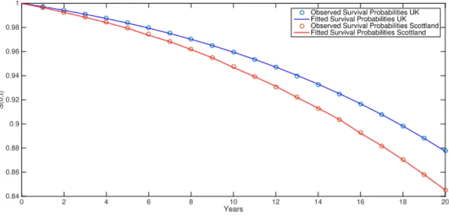
Years 0 2 4 6 8 10 12 14 16 18 20 S(0,t) 0.84 0.86 0.88 0.9 0.92 0.94 0.96 0.98 1
Observed Survival Probabilities UK Fitted Survival Probabilities UK Observed Survival Probabilities Scottland Fitted Survival Probabilities Scottland
Figure 1. Observed and tted survival probabilities for the Reference and the Portfolio Popula-tion.
in the absence of basis risk. We call this a value-at-risk loading principle. Consistently with the above, we implicitly assume that interest-rate risk has already been hedged perfectly or does not exist.
8.1 Calibration
We calibrate the parameters of our Reference (Portfolio) mortality model to the generation of UK (Scottish) males born in 1946, who were aged 64 on
31/12/2010 (i.e. x = 65). Under the constraint given by condition (2), we
x 01/01/1991 as the observation point (individuals have all reached aged 44) and we t the observed survival probabilities Snp(0, t), Spp(0, t) with
t=1,...20. We t our models minimizing the Rooted Mean Squared Error (RMSE) between the model-implied and the observed survival probabilities. We perform two dierent calibrations. The rst calibration ts only the parameters of the Reference Population, using the Human Mortality Database data for UK. The resulting parameters, which are collected - to-gether with the calibration error - in Table 1, are used to simulate the dy-namic Delta-Gamma-Theta hedging strategy without basis risk.
Table 1. Reference Population calibration results.
a b σ Calibration Error
4.13·10−5 0.0709 0.0087 0.00006
Because condition (2) holds, the simulated mortality intensities λnpx (t)
will be strictly positive. In the simulations, we assume that the maximum life-span of an individual belonging to generationxisω= 115, hence the time
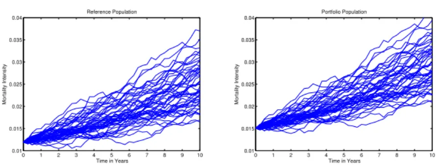
0 1 2 3 4 5 6 7 8 9 10 0.01 0.015 0.02 0.025 0.03 0.035 0.04 Time in Years Mortality Intensity Reference Population 0 1 2 3 4 5 6 7 8 9 10 0.01 0.015 0.02 0.025 0.03 0.035 0.04 Time in Years Mortality Intensity Portfolio Population
Figure 2. On the left-hand side, sample paths of the Reference population intensity process λnpx (t). On the right-hand side, sample paths of the Portfolio population intensity processλppx (t).
second calibration ts the parameters of the Reference and of the Portfolio populations jointly, and is used for the simulations of the dynamic hedging with basis risk. As for the Portfolio population, we use Human Mortality Database data for 65-year-old Scottish males. This population is included in the more general UK dataset and therefore is suitable to act as a sub-population in our example. The calibration error is0.00015, and the values
of the calibrated parameters are shown in Table 2.
Figure 1 shows the observed and the tted survival probabilities for the Reference and the Portfolio populations. Simulated sample paths of both theλnpx (t) and λppx (t) processes are shown in Figure 2.
Table 2. Reference and Portfolio population joint calibration results.
a b σ δx a
0
b0 σ0
3.3357·10−5 0.0727 0.0082 0.9897 0.0077 0.0155 4.4463·10−08
We set the interest rate to a constant valuer = 0.02.
8.2 Rebalancing frequency and dynamic hedging performance without basis risk
In this section we compute the performance of the dynamic hedging strategy we described in Section 7 under dierent rebalancing frequencies. We use the results to assess reasonable ranges for the cost of a longevity swap, as described in Section 6, when basis risk is negligible. Let us consider an annuity provider who has sold a whole-life annuity written on UK males aged 65 at time 0. Three longevity bonds with rolling maturities 10, 15 and 20 years, written on the same generation of 65-year-old UK males, and a risk-free zero-coupon bond with rolling maturity equal to the rebalancing frequency of the dynamic hedge exist.
We evaluate the eectiveness of the self-nancing dynamic Delta-Gamma-Theta hedging strategy xing the time horizon to 30 years. We consider
three dierent rebalancing frequencies of 3 months, 6 months and 1 year, respectively.
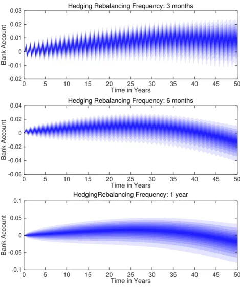
Figure 3 shows the simulated percentiles, from the5th to the95th, of the
distribution of the bank account over time. The value of the bank account is determined, at each rebalancing date, by crediting (debiting) any gain (loss) due to the dierence between the hedging portfolio value before rebalancing and the annuity value.
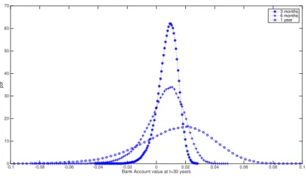
Figure 4 reports the distribution of the bank account after 30 years, for the three dierent rebalancing frequencies. The picture shows that as expected the average cost of the hedging strategy is higher the longer the time interval between two revisions of the strategy. Also, increasing the rebalancing frequency reduces remarkably the dispersion of the value around its mean. The strategy rebalanced at 1-year frequency presents the fattest tails. Table 3 contains, for each case, the mean and standard deviation of the hedging error after30 years and allows to appreciate the eects of dierent
rebalancing frequencies.12
Given the results of our implementation of the dynamic hedging strategy, we compute the cost of the swap based on a value-at-risk loading principle. More precisely, the premium charged to the buyer of the swap C0 is
com-puted as the present value of the 99.5% value-at-risk of the bank account
value att= 30 years obtained applying our hedging strategy with dierent
rebalancing intervals. Table 5 reports the costC0and loadingmof the swap.
The loading m, which represents the percentage increase in each observed
survival, ranges from0.01%to 0.06%. This value might seem low, but it is
a benchmark value, since it is obtained in the absence of transaction costs and basis risk.
3months 6months 1year Mean 0.00073 0.00142 0.00274
Std 0.00068 0.00140 0.00300
Table 3. Moments of the hedging error of the Delta-Gamma-Theta strategy under dif-ferent rebalancing frequencies.
3months 6months 1year Mean 0.00073 0.00142 0.00275
Std 0.00067 0.00143 0.00301
Table 4. Moments of the hedging error of the Delta-Gamma strategy under dierent rebalancing frequencies.
Tables 4 and 6 provide the mean, standard deviations, premiums and loadings for the case in which Theta hedging is not performed. They show that there is not much dierence in terms of results between performing a Delta-Gamma or a Delta-Gamma-Theta hedge. Both strategies provide similar hedging errors, but the Delta-Gamma-Theta requires an additional asset which could increase the overall cost of the strategy if transaction costs were taken into account.
12We remark that this result is obtained in the absence of transaction costs, which we neglect here and will be higher the higher the frequency.
Hedging Rebalancing Frequency: 3 months Time in Years 0 5 10 15 20 25 30 35 40 45 50 Bank Account ×10-3 -4 -3 -2 -1 0 1 2 3 4
Hedging Rebalancing Frequency: 6 months
Time in Years 0 5 10 15 20 25 30 35 40 45 50 Bank Account ×10-3 -8 -6 -4 -2 0 2 4 6 8
Hedging Rebalancing Frequency: 1 year
Time in Years 0 5 10 15 20 25 30 35 40 45 50 Bank Account -0.015 -0.01 -0.005 0 0.005 0.01 0.015
Figure 3. Percentiles of the bank account under dierent assumptions on the hedging rebalancing frequency.
Bank Account value at t=30 years -0.01 -0.008 -0.006 -0.004 -0.002 0 0.002 0.004 0.006 0.008 0.01 pdf 0 50 100 150 200 250 300 350 400 450 500 550 3 months 6 months 1 year
Figure 4. Distribution of the value of the bank account at t=30 years for dierent rebalancing frequencies.
3months 6months 1year C0 0.00209 0.00447 0.01027
m 0.01% 0.02% 0.06%
Table 5. Longevity Swap premiums and loadings equivalent to the99.5%
Value-at-Risk of the Delta-Gamma-Theta Hedging strategy att= 30years.
3months 6months 1year C0 0.00207 0.00470 0.01012
m 0.01% 0.03% 0.06%
Table 6. Longevity Swap premiums and loadings equivalent to the 99.5%
Value-at-Risk of the Delta-Gamma Hedging strategy att= 30years.
8.3 Rebalancing frequency and dynamic hedging performance with basis risk
In this section we examine the performance of a dynamic Delta-Gamma-Theta hedging strategy when basis risk is present. We assume that an annu-ity provider has sold a whole-life annuannu-ity written on Scottish males aged65
at time0. As in the previous section, together with a risk-free zero-coupon
bond, we assume that three longevity bonds written on the generation of65
year-old UK males are traded in the market. The two populations follow now dierent processes, as described in Section 4. Basis risk enters the picture, and a dynamic perfect hedge is not possible.
The hedging error is caused both by the presence of basis risk and by the discrete-time rebalancing of the dynamic hedging strategy. It can be seen from Figure 5 that the bank account is not perfectly centered at zero and that its absolute value is higher than in the case when no basis risk is present, because the idiosyncratic component cannot be hedged. As in the previous case, for each rebalancing frequency, the plot is a fan chart representing the percentiles (from the 5th to the 95th) of the distribution of
Hedging Rebalancing Frequency: 3 months Time in Years 0 5 10 15 20 25 30 35 40 45 50 Bank Account -0.02 -0.01 0 0.01 0.02 0.03
Hedging Rebalancing Frequency: 6 months
Time in Years 0 5 10 15 20 25 30 35 40 45 50 Bank Account -0.06 -0.04 -0.02 0 0.02 0.04
HedgingRebalancing Frequency: 1 year
Time in Years 0 5 10 15 20 25 30 35 40 45 50 Bank Account -0.1 -0.05 0 0.05 0.1
Figure 5. Percentiles of the bank account with basis risk and under dierent assumptions on the hedging rebalancing frequency.
Bank Account value at t=30 years -0.1 -0.08 -0.06 -0.04 -0.02 0 0.02 0.04 0.06 0.08 0.1 pdf 0 10 20 30 40 50 60 70 3 months 6 months 1 year
Figure 6. Distribution of the value of the bank account, under the assumption of basis risk, at t=30 years for dierent rebalancing frequencies.
the bank account. A similar information is conveyed by Figure 6, that shows that the distributions of the bank account are no more centered at zero and present a high degree of asymmetry with long left tails. Table 7 reports the rst two moments of the hedging error of the Delta-Gamma-Theta strategy, at timet= 30years, for each rebalancing frequency. Its mean and standard
deviation are higher than the corresponding moments computed without basis risk (see Table 3). By taking the dierence between the average hedging error in the two cases, we can isolate the part of the hedging error caused by basis risk. For instance, xing the rebalancing frequency at 3 months,
the error due to basis risk is0.00824 = 0.00897−0.00073. We observe that,
though the moments of the hedging error are decreasing in the rebalancing frequency, basis risk is the main determinant of the hedging error, while discrete time rebalancing has only relatively marginal eects.
3months 6months 1year Mean 0.00897 0.01146 0.02362
Std 0.00522 0.00797 0.01657
Table 7. Moments of the hedging error of the Delta-Gamma-Theta hedging strategy, with basis risk, under dierent rebalancing frequencies.
3months 6months 1year Mean 2.08373 2.09597 2.11164
Std 0.20691 0.20715 0.20850
Table 8. Moments of the hedging error of the Delta-Gamma hedging strategy, with basis risk, under dierent rebalancing fre-quencies.
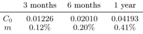
The longevity swap premiums, computed using the value-at-risk load-ing principle, are reported in Table 9. They range now between0.01226and 0.04193, and the corresponding percentage loading on the survival
3months 6months 1year C0 0.01226 0.02010 0.04193
m 0.12% 0.20% 0.41%
Table 9. Longevity Swap premiums and loadings equivalent to the99.5%
Value-at-Risk of the Delta-Gamma-Theta Hedging strategy att= 30years with basis risk.
3months 6months 1year C0 1.48367 1.48762 1.49936
m 14.42% 14.46% 14.57%
Table 10. Longevity Swap premiums and loadings equivalent to the 99.5%
Value-at-Risk of the Delta-Gamma Hedging strategy att= 30years with basis risk.
when basis risk is present, the Delta-Gamma-Theta strategy yield higher costs C0 and spreads m, as expected, but still remains fairly eective. If
we compare the values in Tables 7 and 9 with those in Tables 8 and 10, we immediately see that the Delta-Gamma strategy achieves an hedging error considerably higher than the Delta-Gamma-Theta strategy. Without basis risk the performances of the two strategies were similar but, if basis risk is present, this is no more the case. This result shows that even if hedging when basis risk is not negligible can be eective, the hedging strategy needs to be appropriately designed.
9 Summary and conclusions
This paper introduces a simple model for basis risk in longevity-linked securi-ties, computes the static, customized, swap-based hedge for an annuity, and compares it with the dynamic, Delta-Gamma-Theta based hedge, achieved using indexed longevity bonds. All throughout, the paper assumes a non mean reverting CIR process for mortality intensity. In the theoretical part, we consider interest rate risk as well, while the empirical application focuses on longevity risk only. We show that, once the model is calibrated to a UK individual aged 65, if there is no basis risk the average hedging error of the dynamic hedge is moderate, and both its variance and the thickness of the tails of its distribution are decreasing with the rebalancing frequency. We compute the fee which makes the 99.5% quantile of the distribution of
the dynamic hedging error at an horizon of 30 years equal to the cost of the static hedge. This stays between 0.01 and 0.06%. When there is basis
risk, modelled parsimoniously and consistently, the fee ranges between0.12%
to 0.41%. The same does not hold with simpler Delta-Gamma strategies.
We conclude that, while basis risk is indeed relevant for annuity provider's hedges, dynamic hedging strategies, such as Delta-Gamma-Theta, can still be fairly eective if they are calibrated and implemented appropriately, even when rebalancing occurs at low frequencies. So, even when basis risk is present, a priori, one could rely on dynamic hedging strategies, instead of structuring a fully customized OTC hedge.
as we show that standardized, index-based, products are eective hedges, if appropriately managed.
Robustness of our analysis with respect to dierent populations, annuity features, such as the presence of guarantees, dierent horizons, or longevity model specications, are in the agenda for future research.
References
Barrieu, P., H. Bensusan, N. El Karoui, C. Hillairet, S. Loisel, C. Ravanelli, and Y. Salhi (2012). Understanding, modelling and managing longevity risk: key issues and main challenges. Scandinavian Actuarial Journal (3), 203231.
Blake, D. and W. Burrows (2001). Survivor bonds: Helping to hedge mor-tality risk. Journal of Risk and Insurance, 339348.
Cairns, A. J., K. Dowd, D. Blake, and G. D. Coughlan (2014). Longevity hedge eectiveness: A decomposition. Quantitative Finance 14 (2), 217 235.
Coughlan, G. D., M. Khalaf-Allah, Y. Ye, S. Kumar, A. J. Cairns, D. Blake, and K. Dowd (2011). Longevity hedging 101: A framework for longevity basis risk analysis and hedge eectiveness. North American Actuarial Jour-nal 15 (2), 150176.
Cowley, A. and J. Cummins (2005). Securitization of life insurance assets and liabilities. The Journal of Risk and Insurance 72 (2), 193226. Dahl, M., S. Glar, and T. Møller (2011). Mixed dynamic and static
risk-minimization with an application to survivor swaps. European Actuarial Journal 1 (2), 233260.
Dahl, M., M. Melchior, and T. Møller (2008). On systematic mortality risk and risk-minimization with survivor swaps. Scandinavian Actuarial Journal (2-3), 114146.
Fung, M. C., K. Ignatieva, and M. Sherris (2014). Systematic mortality risk: An analysis of guaranteed lifetime withdrawal benets in variable annuities. Insurance: Mathematics and Economics 58, 103 115.
Haberman, S., V. Kaishev, P. Millossovich, and A. Villegas (2014). Longevity basis risk a methodology for assessing basis risk. Report, Cass Business School and Hymans Robertson LLP.
International Monetary Fund (IMF) (2012). Global Financial Stability Re-port. (IMF April), 123154.
Jarrow, R. and S. Turnbull (1994). Delta, gamma and bucket hedging of interest rate derivatives. Applied Mathematical Finance 1, 2148.
Li, J. and M. R. Hardy (2011). Measuring basis risk in longevity hedges. North American Actuarial Journal 15 (2), 177200.
Luciano, E., L. Regis, and E. Vigna (2012). Delta-gamma hedging of mor-tality and interest-rate risk. Insurance: Mathematics and Economics 50, 402412.
Ngai, A. and M. Sherris (2011). Longevity risk management for life and vari-able annuities: The eectiveness of static hedging using longevity bonds and derivatives. Insurance: Mathematics and Economics 49, 100114. Wong, T. W., M. C. Chiu, and H. Y. Wong (2014). Time-consistent mean
variance hedging of longevity risk: Eect of cointegration. Insurance: Mathematics and Economics 56, 5667.