Farm planning for a typical crop-livestock integrated farm : an application of a mixed integer linear programming model

INTEGRATED

FARM: AN APPLICATION

OF A MIXED INTEGER

LINEAR PROGRAMMING

MODEL

ASSIGNMENT

PRESENTED IN PARTIAL FULFILMENT

OF THE REQUIREMENTS

FOR THE DEGREE OF

MASTERS OF SCIENCE IN OPERATIONAL

ANALYSIS

AT THE UNIVERSITY OF STELLENBOSCH

By

Amanuel Habte Ghebretsadik

December 2004

Supervisor: Professor HC. De Kock

Co-Supervisor:

Mr

S E Visagie

Declaration

I, the undersigned, hereby declare that the work contained in this assignment is my own original work and that I have not previously in its entirety or in part submitted at any university for a degree.

Abstract

In an integrated crop-livestock production farm, the profitability and sustainability of farm production is dependent on the crop rotation strategy applied. Crop rotations have historically been applied to maintain long-term profitability and sustainabiliry of farming production by exploiting the jointly beneficial interrelationships existing among different crop types and the animal production activity.

Monocrop (specifically wheat) growers in the Swartland area of the Western Cape are struggling to maintain long-term profitability and sustainability of the crop production, challenging them to rethink about the introduction crop rotation in the production planning. By making proper assumptions, this paper develops a mixed integer linear programming model to suggest a decision planning for the farm planning problem faced by an integrated-crop-livestock production farmer. The mathematical model developed includes crop production, dairy production and wool sheep production activities, which permitted the consideration of five crop types within a crop rotation system. By assuming that a farmer uses a cycle of at most three years, the crop rotation model was incorporated in the composite mixed integer linear farm planning model.

In order to demonstrate the application of the mathematical farm planning model formulated, a case study is presented. Relevant data from the Koeberg area of the Swartland region of the Western Cape was applied. For each planning period, the model assumed that the farm has the option of selecting from any of 15 cropping strategies. A land which is not allocated to any of the 15 crop rotation strategies due to risky production situation is left as grass land for roughage purposes of the animal production.

Results of the mathematical model indicated that farm profit is dependent on the cropping strategy selected. Additionally, animal production level was also dependent on the crop strategy appl ied. Furthermore, study results suggest that the profit generated from the integrated crop-livestock farm production by adopting crop rotation was superior to profit generated 1'1'0111 the farm activities which are based on monocrop wheat strategy. Empirical results also indicated that the complex interrelationship involved in a mixed crop-livestock farm operation play a major role in determining optimal farm plans. This complex

interrelationships favour the introduction of crop rotation in the crop production activities of the farm under investigation.

Crop production risk is the major risk component of risk the farmer faces in the farm production. In this study, risk is incorporated in the mixed integer

programrnmg

farm planning model as a deviation from the expected values of an activity of returns. Model solution with risk indicated that crop rotation strategy and animal production level is sensitive to risk levels considered. The Results also showed that the incorporation of risk in the model greatly affects the level of acreage allocation, crop rotation and animal production level of the farm.

Finally, to improve the profitability and sustainability of the farm activity, the study results suggest that the introduction of crop rotation which consist cereals, oil crops and leguminous forages is of paramount importance. Furthermore, the inclusion of forage crops such as medics in the integrated crop livestock production is beneficial for sustained profitability from year to year.

Opsomming

Wisselbou is baie belangrik om volhoubare winsgewindheid te verseker in 'n geintegreerde lewendehawe I gewasverbouing boerdery in die Swartland gebied van Wes-Kaap. "n

Monokultuur van veral koring produksie het ernstige problerne vir produsente veroorsaak.

In hierdie studie word 'n gemengde heeltallige liniere prograrnmerings-model gebruik om te help met besluitneming in sulke boerderye.Die wiskundige model beskou die produksie van kontant- en voer-gewasse (5 verskillende soorte) asook suiwel- en wol/vleis-produksie (beeste en skape) .Daar word aanvaar dat die boer "n siklus van hoogstens 3 jaar in die wisselbou rotasie model gebruik ..

'n Gevallestudie word gedoen met behulp van toepaslike data van 'n plaas in die Koeberg gebied. Die model aanvaar dat die produsent 'n keuse het uit 16 wisselbou strategic .Resultate toon dat winsgewindheid afhanklik is van die strategie gekies en dat wisselbou beter resultate lewer as in die geval van "n monokultuur.Dit wys ook dat die wisselwerking tussen diere-produksie en gewasproduksie baie belangrik is in die keuse van 'n optimale strategie.

Die risiko in gewasverbouing is die belangrikste risiko factor vir die produsent.In hierdie studie word risiko ook ingesluit in die gemengde heeltallige model, naamlik as 'n afwyking van die verwagte opbrengs-waardes .Die model toon duidelik dat gewasproduksie en lewendehawe-produksie baie sensitief is ten opsigte van die gekose risiko vlak.

Die studie toon ook dat 'n wisselbou program wat die produksie van graan (veral koring) .oliesade asook voere insluit belangrik is vir volhoubare winsgewindheid Die insluiting van klawers (bv "medics") is veral belangrik hier.

Acknowledgments

First, I wish to thank the Lord for giving me the right direction and guidance throughout my study.

The quality and success of masters thesis research is greatly dependant on the motivation and direction provided by the thesis advisor. Ithas been my privilege to work under the guidance of Professor

He

De Kock, who introduced me to the world of farm planning modelling using mathematical programming models. I wish to thank him for giving me an opportunity to work under him and explore the depths of applications of mathematical programming to agriculture. Thanks, Professor

He

De Kock for your patience, understanding, guidance, support and freedom given in the process of completing this study. I would like to thank my family, without their constant support, encouragement and prayers from the other side of the continent this work would have been extremely difficult. I am very grateful to God for putting such people in my life. Their continued love, affection and prayers have been my pillars of support. Iwould also like to thank the HRD of the University of Asmara, the State of Eritrea for the scholarship SUpp0l1 throughout my study, without the scholarship this study could have not been possible. I am grateful to Ulli & Heide Lehmann for their continuous cooperation and help throughout my study. Finally, a special thanks goes to Heide for proof reading my thesis material tirelessly.

Table of Contents Declaration i .-\ bst racr ii Opsomming iv Acknowledgments y Table of Contents vi List of Ta bles ix List of Figures x Chapter I I Background Information I

I. I ntrod

uction:

Integrated crop

a

nd livestock prod

uction

I

2. Problem Statement and Underlying Assumptions 8

2.1. The Problem 8

2.2. Un derlving Assumptions I()

3.

Underlying Hypothesis and Objectives I...

.... Data 15

5.

Seq uence of Cha pters 16

Chapter

II

18

Literature Review 18

I. Crop Rotation Modelling Background: A Literature Review 18

2.

Rev

iew of Modelling Risk and Uncertainty Using Mathematical

Programming Techniques:

Selected Literature

B

2.1. Game Theoretic Approach 26

2.2. Tile "S(/lf!~1' First" Approach 3...

2.3. The ..

£_, " '.

Approach (Quadratic Progrannning) 37 \ I

2.4. .l/OT-tD -..3

2.5. Target-.l/OT-tD 8

Chapter

111

51

Ma the ma tical Model

51

I.

Introduction

51

2.

Definitions

of Decision

Variables

and Parameters

in the moclel..

5~

.3.

Crop

Rotation

Modelling

55

3.1. Derivation of Crop Rotation Strategies 55

3.2. Limiting .Vul1lha ant! si:« ofStrategies l ntplentented ill the Farm 60

~?~). Land Constraint 63

-t

Income

Variability:

as a Source ofFarm

Risk

6...

5.

Animal

feed activities

68

5./. Blendedfeed (Feed mix) 68

5.2. Roughage Requirements 70

6.

Availability

activities

72

7.

Renting

Activities

7~

8.

Animal

Feed Storage

Constraint

75

9.

Livestock

buying

and selling activities

76

10.

The objective

function

77

Chapter

IV

81

Mathematical

Model

Solution

a nd Sensitivity

A nalysis:

A

Case

Studv ...

81

I.

Introduction

81

2.

Description

of the Agricultural

Activities

of the Farm:

Case Model

Empirical Specification

83

2./. Designitrg Feasible Crop Rotation Strategies and lnput Data Developtnentfor

the .l/athelliatical .llodel 83

2.2. ) >

z.,».

Uairy and Wool Sheep Production Activities 87

-ulditiona! Resource Renting Activities 89

3.

Model Solution

without

Considering

Risk: Com pa rison of

Monocropping

and Crop

Rotation

Farming

Strategies

90

3./. Fanning Plan under .\'orl1lal Year Model Assumption 90

3.2. Fanning Plan utuler Wet Veal' +Iodel Assumption 93

3.3. Farming Plan Assuming all A verage oftlie Three States 95

-to

Model

Solution

with Risk Considerations

98

5.1. .)

s.s.

Sens itivitv .-t1I(/~l'SiS 011 '·(I1I1es of Rish Paratneter 105

Scnsitivitv -uutlvsi« Oil the SIIII/ber of Strategies 107

Sensitivity -tn alysis Oil Price o{ Crops , 108

5.3.

Chapter

V

110

Conclusion

and Future

Studies

110

I.

Conclusion

110

2.

Future

Study

115

Reference

117

Appendix

A: Mixed

Integer

Linear

Programming

Model..

125

Appendix

B: Cost of growing

(Ra nd/hecta

re) Crops

per srrategies

127

Appendix

C: Market

price of crops (Rand/ton)

128

Appendix

D: Yield data (Tons/hectare)

129

Appendix

E: deviation

values

131

Appendix

F: Model

Solution

for Different

values of Risk Levels

132

Appendix

G:

Optimal

Acreage

Allocation

versus

Risk

IJ3

Appendix

H: Model solution

for Different

number

of plots

lJ-t

List of Tables

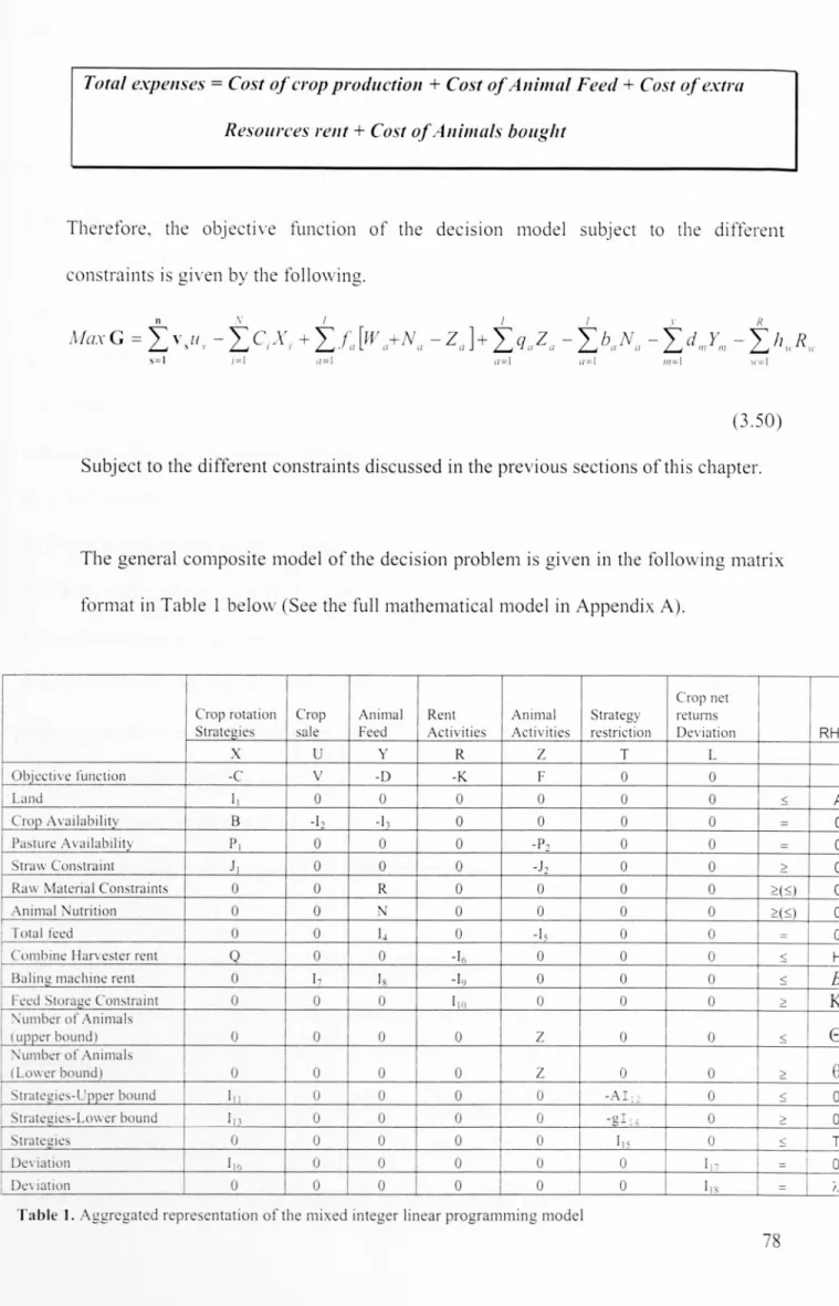
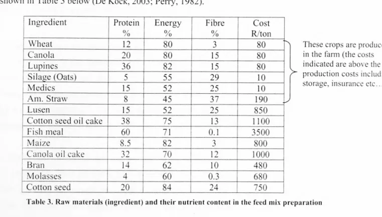
Table 1. Aggregated representation of the mixed integer linear programming model. 78 Table 2. Gross income of the different strategies (Rand/hectare) 86 Table 3. Raw materials (ingredient) and their nutrient content in the feed mix

preparation 87

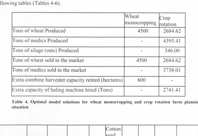
Table 4. Optimal model solutions for wheat monocropping and crop rotation farm

planning situation 91

Table 5. Optimal Feed mix results for animal feeding plan for normal year farming

plan (ton) 91

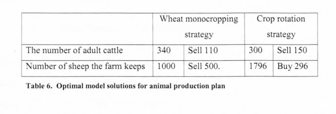
Table 6. Optimal model solutions for animal production plan 92

Table 7. Crop production and sell plan under wheat monocropping farming plan for

wet year scenario 93

Table 8. Optimal Feed mix results for animal feeding plan under wet year assumption

for the monocropping strategy (ton) 93

Table 9. Model solution of wheat monocropping strategy for animal production plan

under wet year assumption 93

Table 10. Optimum crop production marketing plan for the wet year crop rotation

farm production 94

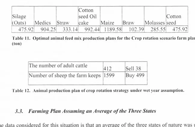
Table II. Optimal animal feed mix production plans for the Crop rotation scenario

farm plan (ton) 95

Table 12. Animal production plan of crop rotation strategy under wet year assumption . ... 95

Table 13. Crop Production and sell plan for average data 95

Table 14. Animal Production Plan 96

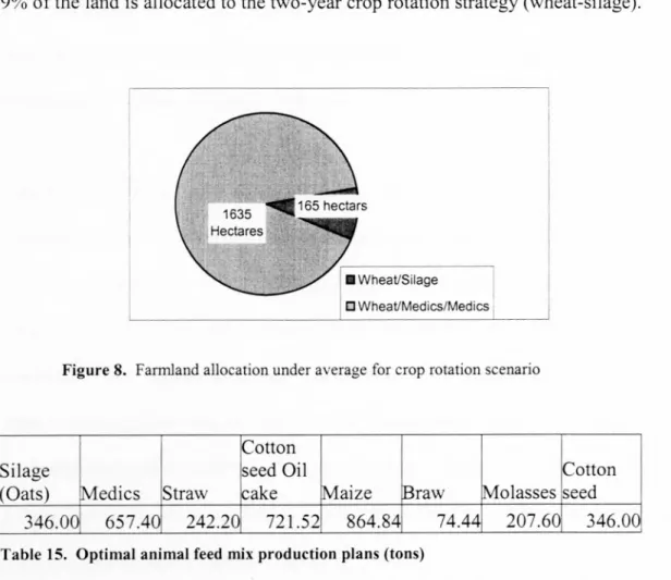
Table 15. Optimal animal feed mix production plans (tons) 96

Table 16. Amount of crops (tons) produced and sold to the market applying the

minimum risk 99

Table 17. Optimal feed mix under minimum risk (tons) 99

Table 18. Optimal animal production plans 99

Table 19. Model solution -quantity of crops (tons) produced and sold to the market for

the constraint level j,=RI,OOO,OOO 100

Table 20. Optimal animal production plans at risk level 1.=Rl,000,000 •••••••••••••••••••••••••• 100

Table 22. Model solution to different risk levels 101

List of Figures

Figure 1. A dynamic cropping system 2

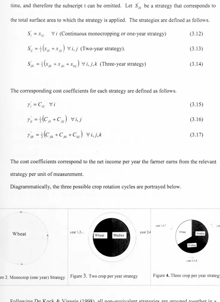
Figure 2, Monocrop (one year) Strategy 58

Figure 3. Two crop per year strategy 58

Figure 4. Three crop per year strategy 58

Figure 5. Two strategies per year farm cropping plan 62

Figure 6. Land allocation under normal year crop rotation scenario 92 Figure 7. Cropping plan under wet year crop rotation situation 94 Figure 8. Farmland allocation under average for crop rotation scenario 96

Figure 9. Farmland allocation for the minimum risk situation 99

Figure 10. Land allocation under A.=Rl,000,000 100

Figure 11. Profit-Risk Frontiers 106

Figure 12. Percentage of acreage allocation for different risk values l07

Chapter

I

Background

Information

1.

Introduction:

Integrated

crop and livestock

production

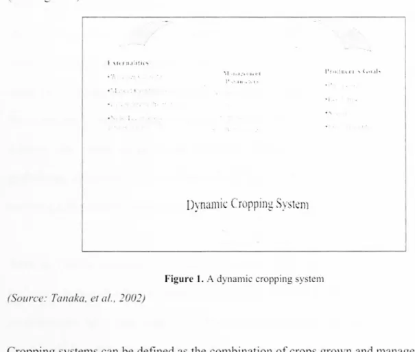
Agricultural activity occurs in an environment that is always changing. In every growing season, producers must pay attention to numerous factors that influence their management decisions. Some factors are within the control of the farmers; however, many are not. The weather, market conditions (including input and output prices), new technology, government policy and information represent some of the factors that have an impact on production decisions. As sustainability and profitability of a farm firm is dependent on the management of these broad categories of externalities, accordingly, the farmer must deal with such factors on a continual basis (Tanaka et al., 2002).

The broad externalities create a daunting task to the farmer who is constrained by many challenging factors. To meet these challenging factors farmers must manage externalities by introducing different management options that optimise the outcome. This is a challenging task. In this regard, producers need to possess the ability to integrate the vast amount of information on externalities that are constantly changing. The information that one needs to understand well enough is how to take advantage of situations in which externalities interact. Furthermore, the information must be translated within the context of the resources available to the producer.

To significantly benefit from the agricultural activities, the modern agricultural production has been and is applying sustainable agricultural management. There are several alternative definitions of sustainable agriculture. However, all seem to agree that the definition includes

reductions in the reliance on non-renewable inputs such as fertilizers and pesticide products; reductions in environmental degradation and an increase in management input (Novak. Mitchell & Crews, 1990; Smit. 1997).

As part of a sustainable agriculture, a practice of dynamic cropping system is of paramount importance for long-term sustainable and profitable farming activity (Tanaka et al., 2002) (See Figure I).

.',\. 1',' 111,.:,1' ,'1 ·1 ... . I ..

Dynamic Cropping System

(Source: Tal/aka, et al., 2002)

Figure I.A dynamic cropping system

Cropping systems can be defined as the combination of crops grown and management applied of which monocropping, intercropping and crop rotation systems are a subset (Harper, 1983; Lockhart & Wiseman, 1988). Crop rotation systems are characterized by a defined sequence of crops grown on a given arable land and the associated management practices.

umerous cropping systems can be technically feasible on a given farmland. However, decision criteria are required to choose among the technically feasible ones. Decision criteria for a cropping system choice can include impact on soil fertility, environmental quality, interdependence with animal acti ities, and of course farm profitability.

Some cropping systems endow the farmer a better profit through their impact on soil quality and fertility. When interest is directed to the long-term sustainability of the agricultural productivity of the farm those social benefits should be valued and incorporated into a decision criterion which is used to compare the various cropping system alternatives. At the farm level, optimising farmers choose the best cropping system from among feasible alternatives. When viewed from the individual farmer's standpoint, farm profitability becomes the overriding criterion. In addition to being technically feasible, a cropping system needs to be profitable to enable survival of the farm as a firm. Annual profits are accumulated over time into retained earnings to enable growth of the farm business. Among the cropping systems, the comparatively more profitable alternatives would still be preferred. The profitability of cropping systems can change over time due to several aspects and farmers need to adopt a sustainable system which is more profitable.

After the 1940's, especially in the developed world, due to the increase in mechanization and the increase in application of chemical protection, farming activities had been tremendously profitable and have been simplified. This simplification has led the farmers to concentrate their production only on one crop type (monoculture practice). According to Harper (1983), the adoption of monoculture practices was prompted due to the following advantages of applying the strategy.

o Simplicity of management

o Reduction in the range of machinery required o Low labour requirement

o Yield levels can be maintained with available fertilizers and crop protection products

However, due to various existing problems in the present agricultural production system, the above mentioned advantages of monocropping are no more relevant to the present agricultural production situation. From time to time the return from monoculture agricultural production is shrinking. The following are some of the factors exacerbating the poor return from monoculture agricultural practices (Harper, 1983).

I. Continuous monoculture cereal cropping does encourage weeds. The control of weeds in the cereal production farming is becoming a problem. Even if

chemicals can be used, control is expensive and difficult. In recent times, the pollution of environment because of such practices is becoming a serious issue. 2. The greater incidence of soil born fungal disease and pest is very difficult to

control.

3. Continuous monoculture cereal growers are more vulnerable to changes in the market trends and prices: The current serious problem of farmers with regard to this is the surplus production of cereals. This results in falling prices of especially wheat and barley.

4. Decline of soil fertility and organic matter: This problem may require additional input of expensive fertilizers. Consequently, the production cost increases making farming activity unprofitable from time to time.

In order to combat the various challenging problems described above, the farming sector has been and is leaning toward applying dynamic cropping system (Tanaka et al., 2002). According to Tanaka et al. (2002), a dynamic cropping system is a long-term strategy of annual crop sequencing that optimises cropping options and the outcome of production, economic and resource conservation goals by using sound ecological management principles. They further described the following key factors of dynamic cropping system.

o Adaptability

o Reduced input cost o Multiple enterprise o Environmental awareness o Information awareness

One of the important aspects of cropping systems can be the employment of effective crop rotation. Taking into consideration the various biological and climatic conditions, careful selection of crop rotation systems offers the possibility of reducing the trade-off between maintaining long-term profitability and reducing environmental impact. Crop rotations are considered as major cropping system alternative to reduce agriculture's dependence on external inputs. This is indirectly achieved by internal nutrient recycling, maintenance of long-term productivity of the land and breaking the weed and disease cycles (Hardy, 1998). Crop rotation is an additional factor that can help rejuvenate the soil as it has several advantages including enhancement of soil fertility and efficient utilisation of plant nutrients. Additionally, crop rotation helps to build soil fertility by not allowing one single type of crop to remove the same nutrients from the soil over a few seasons, as different crops feed on different nutrients at different rates. Growing one crop on the same field over time will result in total loss of many vital nutrients.

The importance of crop rotation has long been recognised prior to the development of modern farming that relied extensively on external inputs. According to the explanation of Struik &

Bonciarelli (1997), the basis of sustainable agriculture is a good rotation, adequate soil, and water management, and proper husbandry of the different crops in the rotation. He further stated that agronomically, farmers should aim at the minimum input of each production resource required to allow maximum utilisation of other resources. Crop rotation serves

multitude purposes including control of pests, weeds, and diseases; reducing soil erosion; maintaining soil fertility and enhancing productivity (Guertal, Bauske & Edwards, 1997; Ikerd, 1991; Hardy, 1998). As dependence on external inputs increased, some believed that the importance of crop rotation would be reduced. However, recent concerns about sustainabiliry of farming profit, environmental impact due to chemical inputs, high rate of use of purchased mineral fertilizers such as nitrogen, acceleration of soil erosion, uncertainty about the long term supply and effectiveness of external inputs and declining yields have brought again crop rotation into the agricultural sector (Ikerd, 1991).

As mentioned above, several advantages of crop rotations have been widely recognised. (Guertal. Bauske & Edwards, 1997). Crop rotations break weed and disease cycles, effectively reduce soil erosion thereby avoiding the long-term decline in the productivity of land and reduce the pollution that could occur otherwise. Crop rotations improve soil quality and improve soil structure thereby enhancing permeability and increase biological activity, increase water storage capacity and the amount of organic matter.

Crop rotations with legumes and oil crops like medics, lupines, canola, and many other types are beneficial to the farm production activity. As most legume types help fix Nitrogen into the soil, introducing legumes in the crop rotation cycle can help to reduce the cost for fertilizer expenses. Moreover, some legumes and oil crops are deep rooted and are excellent for breaking 'Need and pest cycles (Hardy, 1998).

An indirect but important benefit of crop rotation is that it involves diversification. The risk benefit of crop diversification is generally well understood. In an integrated crop-livestock farm environment, diversification reduces risks by spreading among a number of crops and

animals. That is, diversification provides an economic buffer against fluctuations in income resulting from various factors (Alternative agriculture, 1989).

The LIse of crop rotations has generally been thought to reduce risk compared with monoculture cropping (Helmers, Langemeier & Atwood, 1986 cited by Helmers, Yamoah, &

Varvel, 2001). According to Helmers, Langemeier & Atwood (1986), the benefit of crop rotation in reducing risk involves three distinct effects. These are:

[I]. Conventionally practiced rotations involve diversification, which is an offsetting phenomenon where low returns in one year for one crop are combined with relatively high returns from a different crop. [2.] Crop rotation is generally thought to reduce yield variability compared with monocuiture practices. [3]. Crop rotations as opposed to monoculture cropping may result in overall higher crop yield as well as reduced production cost. In addition, assuming that risk is defined as the failure to reach target returns, these influences may reduce risk by reducing the severity of return failures.

To conclude this section, 111 an integrated crop-livestock farm, applying crop rotation is

beneficial to the farmer. Crop rotation is one of the pivotal drivers of sustainable farming. For this reason, introducing crop rotation in agricultural production activity is an indispensable means.

2. Problem

Statement

and Underlying

Assumptions

2.1. The Problem

In many studies dependence on monocropping practices in agricultural production activities and acreage allocations by farmers have been identified as one of the causes of decline in farm profitability. Growing only one type of crop in successive years in a given fixed land has been shown to adversely affect soil structure, cause depletion of organic matter and increase the incidence of diseases, weeds and pest problems. (Hardy, 1998) Furthermore, due to the unpredictability of weather changes, a large portion of instability presents in a yield of a single crop grown.

In consequence, the problem as shown in this paper is one of resource (acreage) allocation decisions by farmers in an integrated crop-livestock crop production farm. There is a need for defining a crop production strategy, which takes into consideration the overall integrated agricultural production system. Given the importance of crop rotation, this paper focuses on risk and diversification issues associated with the selection of crop rotation strategies by taking into consideration dairy and wool sheep production activities of the farm. In addition to the selection of strategies, the decision maker's problem is to integrate the complex relationship existing in the crop and livestock production activities in an optimal manner. Moreover, given the importance of dairy and wool sheep production and the reliance of these production activities in the farmland for some ingredients and pasture requirements, the crop rotation planning is affected by this complex interdependence. In light of this interdependence, the introduction of forage and oil crops in the production planning is of paramount importance to the farmer from economical, biological and ecological perspective (Hardy, 1998).

The second component of the integrated crop livestock production decision problem is the activities of animal production. As part of the farm business, the number of livestock the farm owns is dependent on the availability of the space the farmer has for livestock production and availability of the feed supply. Therefore, as part of the integrated farm-planning problem, determining the number of animals, determining the amount of feed necessary for the livestock's' maintenance satisfying the necessary nutrients and ingredients requirements for both the dairy cattle and wool sheep in the planning period is indispensable.

In this study, it is hypothesised that the farmer owns an agronomically homogeneous fixed area of land. There are II possible crops that can possibly grow on the land. Actually, it is

impossible to grow all types of crops in the fixed land the farmer has. Moreover, it is not profitable and feasible to grow many possible crop types due to management problems, as different varieties of crops need variety of machinery and other tools, tillage practices, etc ... , which make the farm more complex and expensive from small and medium scale farming points of view. Therefore, the farmer's specific problem is then to select a profitable combination of crop and livestock production strategies. That is, the farmer's major problem is to implement cropping strategies that maximise his profit and at the same time minimise risks taking into account the various interlinked activities of integrated crop-livestock enterprise.

In view of the selection of cropping strategies, the farmer's main problem is which strategy to implement monoculture or crop rotation. Considering crop rotation strategies, the farmer is assumed to follow well defined cropping sequences, which do not change from time to time. Under this assumption, farm resources are seen as components of a crop production system where the objective is to exploit the mutually beneficial interrelationships among individual

crops. Accordingly. this cropping scheme provides the vanous benefits described in the

previous chapter; namely: lowering the incidence of weeds, insects and plant diseases; improving soil quality, balancing the requirement for resources and stabilising of the level of farm profits overtime (El-Nazer & McCarl, 1986).

2.2. Underlying Assumptions

The problem described above is a complex one. It requires a clear recognition of the various factors which have an enormous influence in the decision making process of the farm business. Crop production occurs in a complex, biological, agronomical and market dynamics. Since such a complex system offers a formidable challenge to incorporate it into a decision model, representation of such a comprehensive system with a mathematical model is basically not simple. Hence, it is essential to include the following assumptions in the process of developing a mathematical model.

I. It is assumed that the profit, in real terms, remains constant over the period for which the problem is solved. This implies that the cost coefficients in the mathematical model remain constant.

2. The year-to-year variability of the weather conditions of the farm is assumed to be categorised in three discrete states of nature. The three states considered are normal year, dry year and wet year. In this study, these three states of nature are used as the strategies of nature.

3. With reference to the weather conditions with which the decision maker is operating, it is assumed that the farm operates in three possible states of weather conditions. Moreover, the risk of cropping generated from weather variability is modelled as a deviation from the average of the three states of nature.

-t. The profit from a crop is dependent on the crop itself as well as the crop that was planted on the same soil in the previous years. Further, it is also assumed that the crop grown current year is dependent on the crop that was planted on the same soil before two years. However, a crop that grew on the same soil three years ago was assumed to have no effect on the current crop. To highlight this assumption, Wassemann (1982) stated that [as quoted in De Kock & Visagie, 1998)J the cultivation of a specific crop on the specific piece of land may influence the crops that are planted on the same land because of direct (indirect) influences on the level of plant nutrients, on erosion, as well as on the presence of weeds, pests and diseases. In this paper, the influence of crops that grew a year ago or two years ago is reflected in the current crop by the cost coefficients.

5. The most important objective of this study is to develop an optimal sequence of crops to be planted in the farm. In developing this sequence, it is assumed that the optimal sequence of crops form a cycle (El-Nazer &McCarl, 1986; De Kock & Visagie, 1998). For the purpose of this study, only cycles of one, two, and three years will be considered. De Kock & Visagie (1998) presented the following assertions to justify the above assumption.

o The computational effort to solve the mathematical problem rapidly increases as the number of cycles increases. Therefore, it is imperative to limit the number of cycles to a reasonable number that can be handled.

o From the practical perspective of the fanners and the dynamics of the markets, one can argue that the prices of the relevant crops do not remain constant for a long period of time. With this in mind, it is impractical to consider a long cycle, as it is impossible to predict future prices with certainty. Moreover, the longer the cycle is, the higher the chance that price fluctuations will occur so that the current cycle will not be optimal any more.

6. Area of arable land (A) is assumed to be divided into T unit fields (T plots). It is also assumed that the estimated yield of each crop in each field for the specified state of nature is known.

Regarding the complex interdependence between the crop and animal production activities of the farm, the following assumptions are relevant in the farm planning problem.

7. The farm is assumed to be self sufficient in forage and straw production: that is production of forage and straw of the farm must satisfy the animal's consumption requirement for the given planning period.

8. A vai lability in this paper is used in the sense that the animals receive the required amount of feed and roughage which satisfies the ingredient and nutrient restrictions set by the decision maker.

9. For the sake of simplicity, it is assumed that animal sale and buy transaction decisions are made at the start of the planning period. For that reason, animals bought are considered in the animal feed intake planning and animals sold are excluded from the animal feed considerations. Moreover, no activity related profit is generated from those animals sold, as they are assumed out of the activity in the planning period. The only return from these animals is of course the return from the sale of these animals. 10. In this study, animal types are categorised into three sets, namely, adult cattle, young

cattle and sheep. It is assumed that the number of young cattle is always 80% of the adult cattle. Moreover, the only source of revenue from the animal production is revenue from adult cattle and sheep.

I I. The loss from animal death and other natural hazards is assumed to be negligible. Consequently, the cost incurred from such circumstances will not be accounted in the mathematical model.

12. For the purpose of this study. it is assumed that all crops produced at the harvest time are sold or used as animal feed in the feed mix. preparation in the period of study. This implies that no cost is incurred other than the production cost.

13. The variability of input prices is assumed to be negligible. Furthermore, the risk resulting from the variability of input prices in the integrated crop-livestock production will not be investigated. Input risk considerations are beyond the scope of this study. Generally, the cost of different input components of the farm activity for cultivating a particular crop or managing an animal is considered as one grand cost component for each particular activity.

14. The risk of planting crops resulting from unpredictability of weather changes is reflected on the variability of yields of crops in the three nature states. The risk due to this yield variability of crops is shown by the differences in the income variation of the same cropping strategy at the three different states from the expected value.

3. Underlying

Hypothesis

and Objectives

The hypothesis underlying this study is that in an integrated crop-livestock farming em ironment, cropping strategies which rely on crop rotation practices are superior to cropping strategies which are dependent on the practice of monocropping. Further, it is hypothesized that risk affects the choice of resource combination in the farming activity.

The purpose of this study is to point out how the introduction of crop rotation alternatives inf1uence the decision planning of an integrated crop-livestock farm situation in the absence and presence of risk. To investigate both issues, a mathematical model for farm planning will be developed, incorporating the different activities of the farm under consideration.

The more specific objectives of this study are:

I. To determine the optimum maximum profit farm plan which includes an optimum continuously repeatable cropping sequence mix for 1800 hectare of land growing predominantly wheat, canola, silage, lupines and medics; and an optimum dairy and wool sheep production.

2. To investigate the profitability of cropping strategies that employ wheat monoculture and crop rotations.

3. To explore the effect of risk in decision making of the general farming plan by paying special attention to the different cropping strategy alternatives the farmer has.

4. Data

Three sets of data are used in this study. These three sets of data are: 1. Data for the crop production

2. Data for the animal production activities and 3. Data for resources hiring activities of the farm.

The crop production data includes cost of production, price data of crops and yield data of crops for different strategies (see appendix B, C and D). The data are taken from the study taken by Visagie (2004). The crop yield of the five crops, roughage and straw for each of the cropping strategies are presented in appendix D.

The second set of data dealing with the livestock production activities, refer to the annual animal food consumption requirements, nutrient and ingredient restriction. Furthermore, the restriction on the number of animals the farm can keep, profit earned and cost incurred from each type of animal per annum is required to investigate the farm plan. De Kock (2003) and Perry (1982) are used as source of the data used in the model for animal production data req u iremen ts.

The third set of data, which represents the capacity data of the Combine Harvester, and Balling machine the farm owns was taken from De Kock (2003).

5. Sequence

of Chapters

The aspects crop rotation and risk and uncertainty programming modelling from literature are outlined chapter 2. The evolution of crop rotation modelling in the past years will be presented in the first section of this chapter.

Since risk and uncertainty play an important role in agricultural decision making, a brief discussion will be presented in section two of this chapter. Furthermore, section two of this chapter will present a preview of different risk and uncertainty mathematical programmmg models from literature, which are applicable in the farm planning situation.

In chapter 3, a mathematical model for the investigation of the problem stated will be formulated. This chapter consists of 10 sections. Section 1 gives an introduction on the development of a mathematical model. Section 3 will focus on the defining the indices, variables and parameters necessary for the development of the model. In section 3, a mathematical crop rotation model will be developed. Section 4 will introduce risk as a variability of income into the mathematical model as constraint. Sections 5 and 6 focus on the animal feed and availability constraints of the mathematical model. The techniques of mathematical representation of resources renting, storage capacity and animal sale and buy activities are discussed. The final section of this chapter presents the objective function of this study.

Chapter 4 outlines the results of the mathematical model for the problem under investigation. Based on the results of the mathematical model, farming plans for different situations will be analysed. This chapter will present the mathematical model solution solved by WhatsBest' ® 7.0.optimization software. In order to investigate the problem for different farm situations

the mathematical model is soh ed under different assumptions. Section:2 focuses on the development of data used in the mathematical model. Section 3 presents the mathematical model results for the farm plans under assumptions of monocropping and crop rotation for different states of nature conditions without risk. The results of the model \\ hen introducing risk in the model is illustrated in section 4. Sensitivity analysis on the mathematical model for risk, number of strategy and crop prices are examined In section 5.

Chapter 5 deals with a short summary of the study and presents some recommendations future for study.

Chapter

II

Literature

Review

1. Crop Rotation

lVlodeliing Background:

A Literature

Review

According to El-Nazer & McCarl (1986), the economics of rotations have been studied for many years. It was well understood that in order to understand the economic impact of crop rotation in agricultural activities, a mathematical model is required in order to choose the best alternative from the existing feasible alternatives.

The early theoretical discussion of crop rotation selection was done by Heady (1948), as quoted in El-Nazer & McCarl (1986). Following Heady (1948), based on El-Nazer & McCarl (1986) exposition, Hildreth & Reiter (1951) developed crop rotation modelling approaches in one of the first (1949) Linear Programming conferences on Linear Programming applications in USA. In their modelling, they specified alternative linear programming activities as a sequence of crops (rotations). They developed a model to select the optimum combination of crop rotations. Peterson (1955) presented a linear programming model in which crop rotation and a livestock enterprise are selected simultaneously.

One important limitation of the literature on the earliest rotation modelling approaches as

EI-Nazer &McCarl (1986) described, concerns the flexibi lity permitted in the choice of rotations. For instance, all the studies carried out following Hildreth & Reiter (1951) crop rotation modelling define activities in terms of explicit crop sequences. In these studies, the following explicit activity definitions were considered rigidly.

• Three years of com • Three years of hay

• Two years of corn followed by one year of hay • One year of corn followed by two years of hay.

In a similar approach, Beneke & Winterboer (1973) [quoted in EI-Nazer &McCarl (1986)J presented fixed and rigid sequences of crop rotation activities in their example of crop rotation modelling.

The above examples of crop rotation models are based on an explicit configuration of sequences of crops to grow on a given land. As a result of the explicit sequential method of crop rotation modelling, there is a limit in the choice of crop rotations to the combinations that the modeller wants to develop (El-Nazer &McCarl (1986)). Furthermore, model size and data availability considerations are additional limitations of such models. That is, in such modelling approaches one has no freedom of developing different rotation options.

As explained above, historically crop rotations have been modelled using explicit predetermined rotations. To get rid of the limitations mentioned above, Burt (1963, 1982) suggested an alternative approach [as cited in EI-Nazer & McCarl (1986)] defining dynamic programming states provisional on preceding crops.

As pointed out by EI-Nazer & McCarl (1986) the choice of crop rotation model can occur in either a dynamic disequilibrium or a timeless equilibrium setting. In this modelling approach, either multiyear linear programming model (Loftsgard & Heady, 1959; Irwin, 1968; Dean & Benedicts, 1964) as cited by El-Nazer & McCarl (1986)) or the dynamic programming model (Burt & Allison (1963); BUl1 (1956, 1982) cited by El-Nazer & McCarl (1986)) was employed to represent crop rotation in a mathematical model. Both approaches assume the crops chosen in year I to depend on the crops grown in the same land in year I-I. In such

initial conditions. Nevertheless, the models solution tends to stabilize after a few periods. In crop rotations. multi period linear programming models are used to capture the carryover effects of the rotation system on soi I fertil ity, term inal land value overti me, etc... (Baffeo. et al., 1986).

El-Nazer & McCarl (1986) developed a mathematical crop rotation model which allows for rotations to be developed endogenously, with the aims of identifying an optimum long-run crop rotation strategy and its sensitivity to risk attitude. In their modelling approach, they applied an annual, timeless equilibrium model formalized by Throsby (1967) instead of the multiyear linear programming model based on the firm growth model developed by Loftsgard & Heady (1959)[ cited by EI-Nazer &McCari (1986)]. The annual equilibrium approach assumes that the present farming environment should not influence rotation choice; that the interrelationship data are not readily available and that the switch to the optimal rotation was short enough to neglect the time path of adjustment. This alternative modelling approach uses an annual, timeless, equilibrium model. In this case, a continuously repeatable crop rotation is chosen. El-Nazer & McCarl (1986) argued that the solution generated by using this approach corresponds to the stabilised solution of the disequilibrium model and noted that the solutions do not depend on the initial conditions, rather giving a long-term plan.

Clark (1989) developed a linear programmmg model for crop rotation and crop diversification, which is continuously repeatable. Clark's model ignores the agronomic and biological interdependence of crops. That is, the model was built on the assumption that present crop yields are independent of crops grown previously. This is a restrictive assumption, because ignoring the advantages of crop rotation 111 the model can lead into

take different periods to mature and have different yield properties when planted at different dates during a year.

The model was applied to a subsistence farm data from Bangladesh in conjunction with nutrient constraints. The problem was solved using a linear programming code and an optimal solution was generated with another alternative solution. The linear programming solution generated by the model indicates the sequences of crops that can be grown and the optimal planning horizon.

El-Nazer & McCarl (1986) crop rotation model considers II crops and the major assumption

of the model is that the yield of a crop grown in a particular year depends upon the crops grown on the same land in the previous three years. The linear programming rotation model constructed by El-Nazer & McCarl (1986) is represented in the following maximum profit rotation model. II II 1/ 1/ Max

L L L L

c;»

ijkr ;=1 l=' k=1 r=1 1/ 1/ 11 1/ Subject to

LLLLXijkr

< A ;=1 i=1 k=1 /'=1 II 11

LX

ijkr -

LX

ik/,111 ~ 0 for all j = 1,2, ... , n; k = 1,2, ... , n; r =1,2, ... , n (2.1)

X _ijkr ~O

Where ~ikr is the acreage of crop i, which is planted following crops j, k and r in the

preceding years

U

in year t-I, k in year t-2, and r in t-3). Cijkr is the return coefficient in the

objective function in which the objective sums the returns from planting of all possible four-year crop sequences under the total acreage available (A).

El-Nazer & McCarl (1986) stated that the crop rotation constraints (2nd constraint) are the key

elements in the mathematical crop model. Moreover, the timeless equilibrium =continuously repeatable crop plan is an important aspect of the model.

According to the exposition of EI-Nazer & McCarl (1986), the above described mathematical model of crop rotation has been used in a number of studies, particularly in USA and Canada. McCarl et al. (1977) [as cited in EI-Nazer & McCarl, (1986)J used a variant of the model for double cropping where both the preceding crop, and the timing of the preceding crop influence yield. In another study, which is published in the Purdue University Agricultural Experiment Station Bulletin, McCarl (1982) [as cited by EI-Nazer & McCarl (1986)J shows where current return only depends on the immediate preceding crop. The model also includes within year time considerations. The model was also applied by Musser et al. (1981) for vegetation crop rotation modelling, within year crop sequences, double cropping and triple cropping were permitted.

However, due to various factors, the model has a drawback. The major drawback of EI-Nazer

& McCarl (1986) formulation is that the complexity of the model increases enormously with the increase of crops in the model. Particularly, the number of the rotation linkage constraints increases greatly with the increase of the number of crops in the model. Another drawback of the model is the availability of data, namely that it requires a vast set of data.

Built on the same premise as EI-Nazer & McCarl (1986) crop rotation model, De kock &

Visagie (1998) developed a linear programming rotation model under the assumption that optimal sequences of crops form a cycle of three years and shorter. This study will follow the crop rotation model formulated by De Kock & Visagie (1998) in developing strategies of crop sequences for the composite crop -Jivestock mathematical model.

2. Review

of

Modelling

Risk

and

Uncertainty

Using

Mathematical

Programming

Techniques:

Selected Literature

Risk and uncertainty influence the efficiency of resource use in agriculture and decision making process of farmers in their farming activities. Risk is generally considered as a strong behavioural force affecting decision-making. At present, there is much debate amongst theoreticians and applied researchers on research issues related to risk and uncertainty.

The more specific objective of this subsection is to give a partial review on the literature of risk and uncertainty and their modelling aspects. That is, this section is basically a literature review dealing with the general concepts of risk and uncertainty in the agricultural decision making process and gives weight to the review of mathematical programming models which deal with risk and uncertainty modelling. It is not an exhaustive review, and is not intended to be.

Before discussing literatures on risk programming modelling, it is appropriate to define risk and uncertainty. Risk and uncertainty have been defined in different ways depending on the purpose in the mind of the researcher. According to Knight (1921, reprinted in 1965), the distinction between risk and uncertainty is that risk is a condition where probabilities of outcome are known, whereas uncertainty is a condition in which probabilities associated with the outcome are not known. In delineating the degree of knowledge in a decision situation, he further proposed three major categories of decision-making. These are: perfect knowledge, risk and uncertainty. Roumasset (1974) describes this difference as follows: uncertainty is a state of mind, in which the individual recognises alternatives to a particular action. On the other hand, risk has to do with the degree of uncertainty in a given situation. Barry (1984)

draws on uncertainty to indicate imperfect knowledge on the part of the actor and defines risk as the possibility of incurring a loss of production.

The above viewpoints highlight that there is no straightforward agreed definition of risk and uncertainty. However, current popular usage implies that there is very little distinction between risk and uncertainty (Barry, 1984).

Agricultural production is a risky business. Farmers face a variety of price, yield and resource risks, which make their incomes unstable from year to year. Based on an imperfect information, a farm firm makes a decision under price and output uncertainty. The outcomes of a particular decision are revealed ex post, i.e., after the uncertainty is resolved. Since the decision has to be made ex ante (i.e., before the uncertainty is resolved) it has to be evaluated based on ex ante information (Hardaker, Huime, & Anderson, 1997).

Based on Anderson, Dillon & Hardaker (1977), static economic analysis is based on simplified assumptions of certainty about the production environment and an objective of profit maximisation. Linear programrmng models for farm activities are based on this premise. That is, linear programming models are based on expected return rather than sure activity returns. Ideally, the solutions generated by such modelling tools would not satisfy risk-averse farmers. Introduction of risk extends such concepts to include the decision maker's perception of risk and his/her attitude toward risk (Barry, 1984).

The omission of risk in farm level decision models may lead to results that bear little if any similarity to farmers' actual behaviour (Anderson, Dillon & Hardaker, 1977). Agricultural decision models that do not include risk considerations may overestimate outputs of risky activities and fail to recognise the importance of diversification in agricultural productions

systems (Wolgin, 1975). Ignoring risk may also lead to over valuation of some inputs and lead to incorrect prediction of technology choices (Hazell, 1982).

Empirical applications of behavioural models and theoretical considerations indicate the importance of incorporating risk into analysis of agricultural decision making at the farm level. Risk from market, production, environment, and policy factors ... etc will always exist in agricultural decision making (Mapp, et a!., 1979). Subsequently, it is appropriate to take into account risk in agricultural decision making (Anderson, Dillon & Hardaker, 1977; BaITY,

1984).

Various risk-modelling techniques have been developed in the past 40 years to address risk in agricultural decision-making. A number of risk concepts models and their analytical implementation exist in literature (Anderson, Dillon & Hardaker, 1977). Three approaches to risk and uncertainty programming have been reported. Risk and uncertainty concepts and hence, risk and uncertainty mathematical programming models are classified into three major categories: (I) those requiring no probability information or game theoretic models, (2) safety first approaches and (3) expected utility maximisation (Young, 1984). A brief review of the existing major modelling approaches in the evaluation of risky alternatives in agricultural decision-making, which are based on the above categories, follows below.

2. I. Game Theoretic Approach

The conventional game theory formulation is where each player has a number of possible actions, and each set of choices and actions by the players has a consequence, whose 'utility' is typically different for each player. The conventional strategy is that for each player to choose an action for which the worst outcome over all the other player's assignments is best or least bad. This framework can be used to capture uncertainties in agricultural decision-making.

Game theory decision models are one of the main conventional approaches to agricultural decision making under uncertainty (Mclnnerney, 1967 &1969). In this approach, the decision maker's problem is described as a two person zero sum games. All the risk and uncertainty components facing the decision maker can be summarised as a composite 'Nature' component (Hazell & Norton, 1986). Such games are called games against Nature. In the game theory modelling framework a clear definition of nature and the decision maker is important. The following can be cited from Hazell (1970) about the definition of nature.

" ... AIl competitive forces and uncertainty facing a farmer can be summarised as a composite "Nature" component. Thus defined, Nature can be considered an opponent in a two person zero sum games, who, perhaps, randomly rather than wilfully, may financially undo a farmer in his selection of a farm plan, each superimposing its own utility assumptions on the model."

Maltitz (1969) also describes nature as complex and all encompassing opponent as follows. " ... Nature represents the spectrum of uncertainty in the social system and biological complex within which the farmer operates. The farmer has a range

of possible alternative courses of action that he can select a certain combination of enterprises and resource levels. The set of states of nature characterises conditions of weather, resultant prices and other inherent uncertainty phenomena which the farmer can neither control nor predict."

Following Romero & Rehman (1989), the main features of game theory models (game against Nature) can be summarised as follows.

I. The existence of a decision maker (farmer) who is considered as the only rational player of the game.

') The decision maker (farmer) has a set of /I possible sets of strategies or actions to

follow.

3. The existence of a set of li different possible states of nature representing the uncertainties within which the decision maker operates.

4. The game is of the form 11X II matrix whose elements represent the outcome of the

game when the decision maker chooses the ilh strategy to face the TIll state of nature.

As described above, the aim of a game theoretic model is to find a pure or mixed strategy that optimises the wishes and aspirations of a decision maker under different constraints and limitations of resources. This is based on the idea that game theory assumes all important states can be enumerated but avoids an explicit assumption about the probabilities of future occurrence (Hazell, 1970). This approach was introduced to agricultural decision making by Mc1nnerney (1967, 1969). McInnerney (1967) defined a set of available strategies as those that corresponded with feasible set of an ordinary linear programming problem. He defined the payoff matrix of the games as the observed gross margins over a few past years.

A number of criteria have been used to represent the aspirations of a decision maker in the game theoretic model, chiefly in a game against Nature of agricultural planning (Hazell &

Norton. 1986 and Romero & Rehman, 1989). The most prominent of such criteria are briefly discussed in Hazell & Norton (1986) and Romero & Rehman (1989). Some of the well-known criteria's are presented below.

1. The Maxruin (\Vald Criterion)

This criterion assumes that the farmer searches for a strategy, which offers a maximum of the minimum output. That is, the farmer looks for a strategy that maximises the outcome that can be achieved in the worst possible state of nature. In other words, the decision maker examines the worst outcome for each action and then selects the action that maximises the minimum gain from the proposed plan.

In order to represent this criterion in a mathematical model, McInnerney (1969) developed a linear programming model and used this criterion to derive a Maxmin solution for constrained farm planning problem. Following his formulation, the criterion can be represented using the following linear programming model.

MaxZ Subject to CiX~Z

AX{~,~,=}B

(2.2) Where

Z is the worst possible outcome of farm income,

X is the vector of activity levels Xi,

A is the matrix of linear programming coefficients, B is the right hands of the matrix (activity levels),

C; is the vector of the observed gross margin CiT of activity i during state of nature T, T

=

1,2, ... .h

According to the investigation of Hazell and Norton (1986), the Maxmin criterion is very conservative, and often leads to farm plans with such low total gross margins on average in relation to overhead costs and decision maker income needs. As a result, it would not be acceptable to the decision maker. However, they stated that the idea of minimising the worst loss is appealing. Moreover, unlike the E- V models, higher incomes in favourable years are not penalised by the Maxmin decision criterion.

Hazell (1970) and Kawaguchi & Maruyama (1972) independently suggested an addition of an expected income constraint to the Mclnnemey (1969) formulation of the farm planning problem model. This constraint further provides a useful method of analysis to the criterion. Hazell's (1970) parametric formulation of the model is a slight modification of McInnemey's (1969) formulation and is given in the following format.

MaxZ Subject to

CjX;::::Z

AX{~,;::::,=}B

CX=A

(2.3)

Where C is the expected value of

CT

and A. is the target for the expected total farm income. This formulation is an analogue of the Parametric Markowitzean (Freundean) model. The model enables the analyst to draw an indifference curve ), versus Z as was done with the E- V model formulation when an indifference curve was drawn between ), and 02z.

Mclnnemey's (1969) model and its slight modifications have been applied by many authors throughout the world in agricultural decision analysis. Agrawal & Heady (1968), Tadros & Casler (1969), Hazell (1970) and Kawaguchi & Maruyama (1972) are some of the examples.

2. The Minimax Regret (Savage Criterion)

This criterion is based on the assumption that a decision maker wishes to minimise the regret that he/she experiences after having made a decision (Mclnnerney, 1969). The first step in this criterion formulation is the construction of the payoff matrix, called the 'regret matrix'. The elements of this matrix represent the difference between the outcome actually achieved and the maximum outcome the decision maker could have achieved had he known the prices and state of nature that would have prevailed, Based on this matrix, the Savage criterion looks for a strategy which involves the maximum possible "regret" that any state of nature can produce. That is, the Savage regret Criterion focuses on the largest of these regrets over all states of nature and calls for the minimum value of the maximum regret.

The original formulation of this game theoretic decision modelling is given by Mclnnerney (1969); and is given as follows.

Mill V Subject to

s-x

«

V { } [ T = 1,2 ... ,h] A_"y S:,~,=

B

aX =b

xv

» ~

0 (2.4)

Where V is the largest total regret that nature could inflict from any of the !J possible states, R, is the n X m matrix of regrets in which each elements of the regret matrix are calculated as,

In line with McInnerney (1969), this model is designed to identify a feasible farm plan which minimises the largest possible regret that nature could inflict from any of h possible states of nature, through linear programming. However, according to the analysis of Hazell (1970),

Mclnnemey's (1969) model has definite problems. One of the problems mentioned by Hazell (1970) is that optimisation of the programming problem depends on the acreage level. He further points out that McInnerney (1969) assertion is incorrect. The second problem mentioned by Hazell (1970) in the Mclnnerney's (1969) formulation is that the regret component formulation is incorporated into the model due only to the farm constraints rather than to uncertainty. Based on Hazell's (1970) analysis V (largest total regret) has no

meaning.

To take care of the above mentioned drawback, Hazell (1970) introduced the use of direct measure of regret. The direct measure of risk is based on the ordinary linear programming solved for different states of nature. Let gT be the linear programming solution for the problem of the Ttll state of nature. The mathematical representation of the model is given

below. Min V Subject to gr -CrX:S; V

AX{:s;,~,=}B

a'X =b X',V,b~O [r=1,2 ... ,h] (2.5)

Furthermore, Hazell (J 970) proposed the following parametric linear programming adaptation of the Maxmin criterion for farm planning

Mill V Subject to a

-C

X < V Orr

-AX{:s;,~,=}B

CX =)c [T =1,2 ... ,h] (2.6)

In the above formulation, )I_ is parameterised to provide an efficient income (E) and regret (V)

3. The Benefit Criterion

Agrawal & Heady (1968) have argued that Wald's Maxrnin criterion is pessimistic leading to a conservative solution. On the other hand, according to their analysis of Savage's criterion, it is optimistic leading the decision maker to choose a risky solution. As alternative to both approaches, Agrawal & Heady (1968) offered "The Benefit criterion" which combines the properties of both Wald's criterion and Savage's criterion.

In this approach, the benefit matrix is formulated from the payoff matrix. The elements in this matrix represent the differences between the outcome actually received by the decision maker and the minimum he/she could have achieved under the worst state of nature. The next step in this approach is the selection of a strategy that maximises the minimum possible benefit under any state of nature. The Benefit criterion is less optimistic than the regret criterion and less pessimistic than the Wald's criterion, based on the argument of Agrawal & Heady (1968).

The above discussed class of models requiring no probability information are commonly referred to as game theoretic models. These types of models assume that decision makers have no objective information or subjective feeling about the probabilities associated with alternate outcomes. On the other hand, they totally ignore whatever information the decision maker may have. The main criticism of such models stems from this point of view. Anderson, Dillon & Hardaker (1977) explain that such models can be criticised on the ground that the decision criteria employed are incompatible with the axioms of rational choice underlying decision analysis.

Game against Nature models assume that nature acts as a conscious opponent of a decision maker, that IS it strives to limit the expected payoff to the minimum. Such a viev, may suit to

pessimistic or cautious decision maker, but may not be attractive to an optimistic decision maker. Critics argued that assumption that Nature is malicious is not possibly accurate, According to Kmiettowicz & Pearman (1981) description, Nature neither consciously fax ours a decision maker nor hinders him. As a result, the application of such models is fairly limited in the farm planning modelling,

2.2. Tlte "Safety First" Approach

According to Robinson, et.al (198-+), the safety first approach to risk programming is commonly used in risk analysis as a form of lexicographic utility. To be precise, this approach to risk management is applicable if a decision problem aim is first to a preference for safety (such as minimising the probability of bankruptcy) when making decisions in the agricultural activities. This means that only when the safety goal is met at a threshold level the other goals can be addressed. Thus, the highest priority goal serves as a constraint on goals that have successfully lower priorities (Bigman, 1996).

Safety-first mathematical programming methods are particularly applicable where survival of the business is of paramount concern. However, in most business risk management situations, the use of safety-first methods is somehow arbitrary, as no single goal can be clearly dominant from a set of goals the firm has.

As explained by Robinson et al. (1984), the safety first criterion can be specified in various ways of empirical formulation. The first type was introduced by Telser (1955). As described in Robinson et al. (1984), this method assumes that the decision maker maximises expected return (E(y» subject to the constraint that the probability of returns less than or equal to a specified disaster level (Yl11illil11ul11) does not exceed a given probability. Mathematically

Telser's (1955) approach is expressed as follows. /11/(IyE(r)

The second safety-first approach was introduced by Kataoka (1963). This approach selects a plan that maximises return at a lower confidence limit (L) subject to the constraint that the probability of return being less than or equal to the lower limit does not exceed a specified value of probability. (Robinson et al (1984)) Mathematically.

MarL

such that (2.8)

Prob(E(Y) < L) ~ P

The third type of safety-first approaches was developed by Roy (1952), as described in Robinson, et al (1984) and involves choosing the set of activities with the smallest probability of yielding an expected retum below a specified disaster level of return (Yl11in).

Mathematically this approach can be expressed as in the following format. min

peE

< EJ11il1)

(2.9)

The topics that have been addressed by the above mathematical modelling approaches of the safety-first method vary widely. Optimal Hedging (Telser, 1955), Dynamic cropping decisions (van Kooten, Young & Kran, 1997), farm extension programs (Musser, Ohannesia

& Benson, 1981), attitudes toward risk regarding fertilizer applications among peasants in Mexico (Moscardi & Janvry, 1977), a discrete stochastic farm management model with chance constraints to access the risk-income tradeoffs associated with buying, selling and producing at alternative fish growing stages (Hatch, Atwood, & Segar, 1989) are some of the topics investigated by such risk programming model ..

The drawback of the first and second safety-first approaches is that they are not generally compatible with the general utility theory (Bigman, 1996). According to the explanation of Bigman (1996), these safety first criteria need not satisfy the continuity and independence

axioms. Even though the third approach (Roy's criterion) can be derived from a utility function, Bigman (1996) pointed out that in general this approach does not strictly rise with a rise in safety threshold.