detection of brain activity with electrical
impedance tomography
N. Polydorides, W.R.B. Lionheart and H. McCann
2002
MIMS EPrint:
2006.240
Manchester Institute for Mathematical Sciences
School of Mathematics
The University of Manchester
Reports available from:
http://www.manchester.ac.uk/mims/eprints
And by contacting: The MIMS Secretary School of Mathematics The University of Manchester Manchester, M13 9PL, UK
Krylov Subspace Iterative Techniques: On the
Detection of Brain Activity With Electrical
Impedance Tomography
Nick Polydorides, William R. B. Lionheart, and Hugh McCann*
Abstract—In this paper, we review some numerical techniques
based on the linear Krylov subspace iteration that can be used for the efficient calculation of the forward and the inverse elec-trical impedance tomography problems. Exploring their compu-tational advantages in solving large-scale systems of equations, we specifically address their implementation in reconstructing local-ized impedance changes occurring within the human brain. If the conductivity of the head tissues is assumed to be real, the pre-conditioned conjugate gradients (PCGs) algorithm can be used to calculate efficiently the approximate forward solution to a given error tolerance. The performance and the regularizing properties of the PCG iteration for solving ill-conditioned systems of equa-tions (PCGNs) is then explored, and a suitable preconditioning ma-trix is suggested in order to enhance its convergence rate. For image reconstruction, the nonlinear inverse problem is considered. Based on the Gauss–Newton method for solving nonlinear problems we have developed two algorithms that implement the PCGN iteration to calculate the linear step solution. Using an anatomically detailed model of the human head and a specific scalp electrode arrange-ment, images of a simulated impedance change inside brain’s white matter have been reconstructed.
Index Terms—Brain activity, computational efficiency,
conju-gate gradients, electrical impedance tomography, regularization.
I. INTRODUCTION
I
N ELECTRICAL impedance tomography (EIT) a number of low-frequency current patterns are injected from the bound-aries of a conductive volume by some electrodes while a number of linearly independent voltage measurements are captured on others. The imaging capabilities of EIT are based on the fact that the knowledge of an adequate set of boundary measurements along with an accurate model of the volume and some prior in-formation can be used to reconstruct the electrical conductivity distribution in the interior of the volume at the time when the measurements were captured.One of the most challenging projects involving EIT is the de-tection of brain activity under some physiological phenomena that are known to cause local and temporal conductivity changes within the human brain tissue [3]. Classical examples are the
Manuscript received August 28, 2001; revised February 22, 2002. Asterisk
indicates corresponding author.
N. Polydorides is with the Department of Electrical Engineering and Elec-tronics, UMIST, M60 1QD Manchester, U.K.
W. R. B. Lionheart is with the Department of Mathematics, UMIST, M60 1QD Manchester, U.K.
*H. McCann is with the Department of Electrical Engineering and Elec-tronics, UMIST, P.O. Box 88, M60 1QD Manchester, U.K.
Publisher Item Identifier 10.1109/TMI.2002.800607.
visual and auditory stimuli [21] as well as several ambulatory cases like migraines, strokes and epilepsy [4], [14], [19]. De-spite the fact that the effects of these conditions vary in their magnitude and duration, each one tends to affect a particular area of the brain. This paper is primarily focused on the brain response to visual stimulation seeking to explore how this can be accurately and efficiently recovered in the prospect of a robust and reliable on-line monitoring based on EIT. In [15], Holder et
al. have reported that the conductivity changes caused by this
form of stimulus lie in the range 2.7%–4.5%, and as such these are small enough to allow the consideration of a linear approx-imation to the nonlinear inverse conductivity problem.
For a conductive volume of fixed boundaries and a certain conductivity distribution, the forward problem requires the calculation of the potential distribution inside the volume when known current patterns are injected from its boundaries. The mathematical modeling of the forward problem incorporates an elliptic partial differential equation derived from Maxwell’s equations in the low-frequency range and some mixed boundary conditions [8]. The problem is often solved numerically rather than analytically using finite-element approximations, which necessitate a finite-element model of geometrical and structural characteristics similar to those of the real volume. Neglecting any magnetization effects, when the volume is a linear and isotropic medium with boundary , the physical system is governed by the following set of equations also known as the complete electrode model (CEM) [25]. If is a point in the volume, then
(1) (2) (3) (4) In the above equations, is the potential distribution inside , is the contact impedance of the th electrode , is the potential measured on , and is the current injected by and the outward unit normal. For the same equations, denotes the surface underneath the electrodes, denotes the rest of the boundary, and denotes the electrical conductivity which is taken as real and positive. Formulating the variational-Galerkin form of the forward problem as in [20] and adopting a
element method (FEM) approach, the forward problem can be expressed as a system of linear equations
(5) In a system with electrodes attached at the boundaries of a mesh incorporating nodes and elements, if , then is the sparse, symmetric and positive definite global conductance matrix, is the approximated po-tential distribution, and is the associated low-fre-quency current patterns. The existence and uniqueness of the solution are preserved by incorporating into the model some ad-ditional constraints regarding the applied currents and measured
voltages. In effect, and are imposed
[20]. The solution of the forward problem can be naively at-tempted using a conventional method like the Gaussian elim-ination with pivoting for instance, although usually more effi-cient techniques like the Cholesky method [22] are employed exploiting the symmetric structure of the matrix .
II. CONJUGATEGRADIENTS(CGs)
The CGs iteration as a technique for solving linear systems is based on the idea that a problem of a certain dimension can be projected into a lower dimension Krylov subspace [12]. In doing so, the original problem is effectively reduced to a sequence of lower dimension matrix problems. When applied to the system of equations (5) the solution obtained by the th iteration will lie in the associated Krylov subspace generated by and , like
where
span (6)
The algorithm originally derived from the Lanczos iteration [10], requires the coefficient matrix to be sym-metric and positive definite, thus, it can only be applied in EIT’s forward computations when the conductivity is real. Nevertheless, there are other Krylov subspace methods [2], [10] that are suitable for solving systems of equations where the coefficient matrix is likely to have complex or negative eigenvalues. Setting an initial estimate of the solution , the CG algorithm applied to the system (5) can be described as
where is the step length, is the residual vector, is the search direction, and is the approximate solution at the th
iteration. If is the error tolerance parameter, then the iterations progress until the condition is satisfied. From the definition of , an important concept involved in this technique is the -norm of a nonzero vector , which according to [22] is defined as
(7) thus, must be square and positive definite. The fundamental principle behind the CG iteration is that instead of minimizing the two-norm of the residual , the -norm of the error func-tion is minimized, where is the exact solu-tion of the forward problem such that . In this sense, while the iterations are progressing, a unique sequence of iter-ates is generated with the property that at iteration , the -norm of the error is minimized.
When dealing with real experimental measurements the ac-curacy of the forward calculations is often set by the precision of the measurement circuit, i.e., the error estimate in the actual measurements. As the system described in (5) is a discrete ap-proximation, will be an approximate solution strongly de-pending on the quality and the smoothness of the finite-element model used. Setting appropriately the error tolerance parameter , the CG algorithm enables the calculation of the solution based on “how accurately” one aims to solve the system avoiding any unnecessary refinement computations. From the description of the algorithm, one can notice that the solution update is gen-erated by moving a distance in the current search direction. In addition, throughout the iterations the search directions and residual vectors maintain certain properties. More specif-ically, after iterations the residual vectors form the orthogonal basis and the search directions are found to be mutually “ -orthogonal.”
III. CONJUGATEGRADIENTSPRECONDITIONING
The efficiency of the CG algorithm when applied to linear systems is critically dependent on the eigenvalues of the coeffi-cient matrix. In the optimum case, these will be clustered around a fixed positive number and, therefore, a few iterations will be adequate for the algorithm to reach convergence. The concept of preconditioning is based on the idea that one can drastically im-prove the properties of the coefficient matrix before the begin-ning of the iterations and consequently eliminate the computa-tion time required. For an appropriately selected precondicomputa-tioner , the forward problem described in (5) has a solution that is identical to the one of the system
(8) only in this case the convergence of the algorithm will depend on the properties of rather than those of alone. A left preconditioner is regarded suitable when it is positive definite
and the factor satisfies , condition ( )
condition ( ) where is the identity matrix. A quite popular and efficient preconditioning option is the one arising from the incomplete Cholesky factorization of [10]. If is the upper triangular factor of , then a preconditioner is formed such as preserving the existence of a unique symmetric
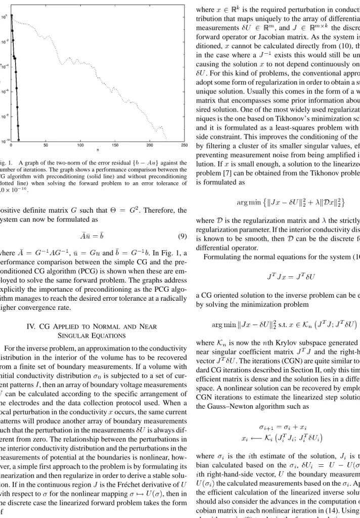
Fig. 1. A graph of the two-norm of the error residualfb 0 Aug against the number of iterations. The graph shows a performance comparison between the CG algorithm with preconditioning (solid line) and without preconditioning (dotted line) when solving the forward problem to an error tolerance of 1.02 10 .
positive definite matrix such that . Therefore, the system can now be formulated as
(9)
where , and . In Fig. 1, a
performance comparison between the simple CG and the pre-conditioned CG algorithm (PCG) is shown when these are em-ployed to solve the same forward problem. The graphs address explicitly the importance of preconditioning as the PCG algo-rithm manages to reach the desired error tolerance at a radically higher convergence rate.
IV. CG APPLIED TO NORMAL AND NEAR
SINGULAREQUATIONS
For the inverse problem, an approximation to the conductivity distribution in the interior of the volume has to be recovered from a finite set of boundary measurements. If a volume with initial conductivity distribution is subjected to a set of cur-rent patterns , then an array of boundary voltage measurements can be calculated according to the specific arrangement of the electrodes and the data collection protocol used. When a local perturbation in the conductivity occurs, the same current patterns will produce another array of boundary measurements such that the perturbation in the measurements is always dif-ferent from zero. The relationship between the perturbations in the interior conductivity distribution and the perturbations in the measurements of potential at the boundaries is nonlinear, how-ever, a simple first approach to the problem is by formulating its linearization and then regularize in order to derive a stable solu-tion. If in the continuous region is the Fréchet derivative of with respect to for the nonlinear mapping , then in the discrete case the linearized forward problem takes the form of
(10)
where is the required perturbation in conductivity dis-tribution that maps uniquely to the array of differential voltage
measurements , and the discrete linear
forward operator or Jacobian matrix. As the system is ill-con-ditioned, cannot be calculated directly from (10), thus, even in the case where a exists this would still be unbounded causing the solution to not depend continuously on the data . For this kind of problems, the conventional approach is to adopt some form of regularization in order to obtain a stable and unique solution. Usually this comes in the form of a weighting matrix that encompasses some prior information about the de-sired solution. One of the most widely used regularization tech-niques is the one based on Tikhonov’s minimization scheme [8] and it is formulated as a least-squares problem with an extra side constraint. This improves the conditioning of the Jacobian by filtering a cluster of its smaller singular values, effectively preventing measurement noise from being amplified in the so-lution. If is small enough, a solution to the linearized inverse problem [7] can be obtained from the Tikhonov problem which is formulated as
(11) where is the regularization matrix and the strictly positive regularization parameter. If the interior conductivity distribution is known to be smooth, then can be the discrete form of a differential operator.
Formulating the normal equations for the system (10) as (12) a CG oriented solution to the inverse problem can be evaluated by solving the minimization problem
s.t. (13)
where is now the th Krylov subspace generated from the near singular coefficient matrix and the right-hand-side vector . The iterations (CGN) are quite similar to the stan-dard CG iterations described in Section II, only this time the co-efficient matrix is dense and the solution lies in a different sub-space. A nonlinear solution can be recovered by employing the CGN iterations to estimate the linearized step solution within the Gauss–Newton algorithm such as
(14a) (14b) where is the th estimate of the solution, is the
Jaco-bian calculated based on the , is the
th right-hand-side vector, the boundary measurements and the calculated measurements based on the . Apart from the efficient calculation of the linearized inverse solution, one should also consider the advances in the computation of the Ja-cobian matrix in each nonlinear iteration in (14). Using the PCG algorithm as in (9) to obtain the forward solutions required for the calculation of will effectively improve the efficiency of
the whole nonlinear algorithm. Using an adjoint problem for-mulation [5], [7], the update of the Jacobian can be cal-culated as
(15)
where , are the field solutions calculated based on the th conductivity distribution update and the th and th current pat-terns, respectively. It must also be quoted that techniques like the adjoint source method [1] can help forming factors very efficiently.
The intrinsic regularizing properties of the CGN algorithm [2], [12] can be easily verified. Although in principle the iter-ations target to minimize the -norm of the error function, in effect they cause the two-norm of the residual to be min-imized. If , then modifying (7) and solving for the error shows that after iterations the condition
minimum is satisfied. In this case, if is the actual inverse so-lution and is the error norm such that , then as the iterations progress the function can be shown to be minimized
constant where
From the above, one may conclude that after iterations
minimum over (16)
Some simple algebra reveals that can also be expressed as
(17) from which it follows that the th iterate minimizes over the same subspace. In addition, since
(18) the value of for which is minimum is also an approximate solution to the ill-conditioned system (12) [10].
V. IMPLEMENTATIONISSUES
Preconditioning properly the CGN iterations can cause dramatic improvements to their computational efficiency in the sense that a lower condition number will enable a higher convergence rate. For this reason, the diagonal matrix
was selected, which despite having quite small singular values its condition number is radically smaller compared to the one of the matrix as these are maintained
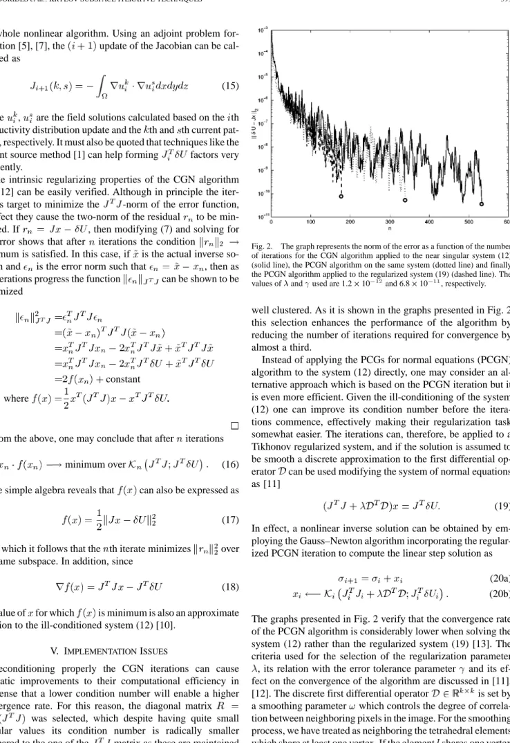
Fig. 2. The graph represents the norm of the error as a function of the number of iterations for the CGN algorithm applied to the near singular system (12) (solid line), the PCGN algorithm on the same system (dotted line) and finally the PCGN algorithm applied to the regularized system (19) (dashed line). The values of and used are 1.2 2 10 and 6.82 10 , respectively.
well clustered. As it is shown in the graphs presented in Fig. 2 this selection enhances the performance of the algorithm by reducing the number of iterations required for convergence by almost a third.
Instead of applying the PCGs for normal equations (PCGN) algorithm to the system (12) directly, one may consider an al-ternative approach which is based on the PCGN iteration but it is even more efficient. Given the ill-conditioning of the system (12) one can improve its condition number before the itera-tions commence, effectively making their regularization task somewhat easier. The iterations can, therefore, be applied to a Tikhonov regularized system, and if the solution is assumed to be smooth a discrete approximation to the first differential op-erator can be used modifying the system of normal equations as [11]
(19) In effect, a nonlinear inverse solution can be obtained by em-ploying the Gauss–Newton algorithm incorporating the regular-ized PCGN iteration to compute the linear step solution as
(20a) (20b) The graphs presented in Fig. 2 verify that the convergence rate of the PCGN algorithm is considerably lower when solving the system (12) rather than the regularized system (19) [13]. The criteria used for the selection of the regularization parameter , its relation with the error tolerance parameter and its ef-fect on the convergence of the algorithm are discussed in [11], [12]. The discrete first differential operator is set by a smoothing parameter which controls the degree of correla-tion between neighboring pixels in the image. For the smoothing process, we have treated as neighboring the tetrahedral elements which share at least one vertex. If the element shares one vertex
with the elements , then the corresponding entries in the matrix are
(21) Another alternative approach to the algorithm (14) is to modify the PCGN iteration in a way that the computational efficiency is not compromised by the size of the the normal equations coefficient. As it appears from the (12) and (19) the coefficient matrix where is the number of mesh elements, dominates the computational complexity of the system. To overcome these computational limitations a modified version of the PCGN algorithm [10] can be employed where by introducing the dummy variable the compu-tationally expensive system (12) is transformed as
(22a) (22b) (22c) In this case, the PCGN iterations are applied to the system (22b) solving for until the desired tolerance is reached. The value of at which the algorithm finally converges is then used to calcu-late the associated value of as in (22c). If is an initial guess for the solution of the system (22b) and the preconditioning matrix such as , the modified PCGN iteration can be described as
where is the error tolerance. From the above description, it is obvious that the value of that minimizes the residual
also minimizes as the two residual vec-tors and can be easily proved to be equal. This modified version of the PCGN algorithm can also be used within the Gauss–Newton method to form an efficient nonlinear solver for the underdetermined problem such as
(23a) (23b) (23c)
TABLE I
THECONDUCTIVITYVALUESASSIGNED TO THEHEADTISSUES IN m , ALONGSIDE THENUMBER OFELEMENTSENCAPSULATED INEACH
OF THEMODELTISSUES
In problems where bulky models are involved, the compu-tational efficiency becomes a crucial issue for the reconstruc-tion. The large number of mesh elements is often the reason that compromises the inverse computations on moderate machines, however, under certain conditions these can be radically sim-plified [1]. Consider for instance the situation where two
dis-tinct volumes and form the measurement
volume in a way that . If all the possible con-ductivity changes can be solely confined within say , one can truncate the domain of the discrete forward mapping (10) in a way that only the columns referring to the elements of are included in the inverse computations. Restricting the range of the inverse problem by avoiding to calculate the solution where we are confident about its value maintains the Jacobian matrix within easily handled sizes and the time required for the com-putation of the solution within reasonable levels. In the anatom-ically detailed model employed in this study, the majority of the elements are allocated in tissues whose electrical properties are unlikely to change during the controlled conditions that we in-vestigate. Tissues like the skin and the skull for instance, which encapsulate almost 67% of the overall number of elements, can be safely regarded as passive as these are expected to maintain their conductivity constant throughout the measurement acqui-sition process [16].
VI. SIMULATEDRESULTS
To perform the simulations we have used a three-dimensional (3-D) model of the human head constructed based on the infor-mation provided by the visible human project [26], comprising 9047 vertices connected in 44 304 first-order tetrahedral ele-ments. Although the skull and the white matter are known to be anisotropic [9], in this paper we regard all the tissues involved as linear isotropic media. The conductivity values assigned to them are summarized in Table I [18], [21].The specific brain area tar-geted in this application is the visual cortex which is mainly con-sisted of the primary visual area and the visual association area. In this case, we have simulated a local conductivity increase of 4% within the occipital lobe, slices of which appear at the left side of the Fig. 4. This inhomogeneity can be considered to be equivalent to the effect of the visual stimulation on a heavily anaesthetized human subject [15].
A number of previous studies [17] have reported on the performance of single plane electrode systems in applications involving volumes of complicated geometrical and structural characteristics, emphasizing the effects caused by the absence of 3-D measurements on both the quality of the reconstructed image and the convergence of the reconstruction algorithms.
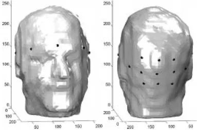
Fig. 3. The 16 electrodes attached on the human head. Views of the arrangement from the front and the back.
The number and the positioning of the electrodes on the head’s surface are among the issues where practical limitations are likely to arise. Although in principle one would aim to maxi-mize their number, locating them throughout the surface of the scalp, a large number of electrodes and consequently a large number of measurements, will introduce delays in both the data acquisition cycle and the image reconstruction as the size of the problem will grow. In this concept it is also important to consider the relation between the data acquisition cycle and the “lifecycle” of the targeted effect. In real experiments, prolonged measurement cycles that are likely to occur in the presence of multiple current patterns, may distort the measurements because the magnitude of the particular effect is rather fast and periodic [16]. Unless time-varying models are adopted it is imperative that each measurements gathered refers to the same conductivity distribution, thus, the duration of the data acquisition cycle is a crucial factor if we are to consider the physiological effect static while the measurements are captured [24].
To meet the above specifications, a 3-D 16-electrode config-uration was developed aiming to allow: 1) suitable current pat-terns to penetrate the resistive skull setting up an adequate field in the interior; 2) linearly independent multiplane measurements between closely located electrodes; and 3) the collection of the majority of the data from the boundary surface near the partic-ular area of interest, i.e., the back area of the head. In order to pass an adequate electric current through the relatively high-re-sistive skull, among others some current patterns from diametri-cally located electrodes were also injected. In addition, care was taken to place some of these electrodes close to the eye sockets and ear holes, exploiting skull’s structural characteristics. As far as the measurement patterns are concerned, most of the elec-trodes have been deliberately placed at the back area of the scalp close to where the the targeted effect was “expected” to occur, in order to enhance the system’s sensitivity in that particular re-gion. The exact positions of the 16 electrodes on the scalp are those indicated in Fig. 3. From this arrangement, a total of 19 current patterns were injected and 369 boundary voltage mea-surements were obtained by forward calculations. To perform the simulations in realistic conditions where the measurements
are contaminated with a certain amount of noise, the measure-ments were infused with a Gaussian noise signal of zero mean and standard deviation of 10 of the norm of the measure-ments. This form of noise can be easily associated with the in-strumentation noise introduced by the data acquisition circuit [6].
In order to be able to provide some form of assessment to the results obtained, one must consider what characteristics a suc-cessfully reconstructed image should possess, mainly in terms of its spatial resolution and its utility for medical diagnosis. Based on the particular simulated inhomogeneity, an acceptable image should indicate a single conductivity increase, symmet-rically situated at the back side of the head, bounded within the brain matter tissue, and having geometrical characteristics sim-ilar to those of the simulated inhomogeneity. The images pre-sented at the left column of Fig. 4 indicate the exact location of the simulated impedance change in slices deployed throughout the inhomogeneity’s volume. The relevant slices from the 3-D nonlinear inverse solution, which corresponds to an error norm of 1.26 10 are those appearing at the right column of the same figure. The images are extracted from the solution ob-tained by the third Gauss–Newton iteration using the PCGN al-gorithm to compute the linearized step as in (20). The recon-struction shows a localized impedance increase of magnitude similar to the one of the simulated change, situated at the back area of the brain matching the position where the original inho-mogeneity has been simulated. Despite the presence of the re-sistive skull, the change has been successfully detected having most of its geometrical characteristics (symmetry and boundary shape) transferred into the image. In terms of its spatial reso-lution, the reconstructed change appears to fit reasonably well within the boundaries of the simulated one. As the system is heavily underdetermined the attempt to solve the problem with
degrees of freedom using a radically smaller set of data will cause a systematic correlation among the elements of the solution that correspond to nearby pixels. As a result, when the solution is projected on to the pixels a smoothing effect is ob-served. The nonlinear inverse problem was attempted using both of the PCGN-based approaches described in Section V. At first, the Gauss–Newton PCGN algorithm was applied to the regular-ized system as in (20) using as preconditioner the
matrix, while the problem was later solved using the underde-termined version of the PCGN algorithm (23) preconditioned with the diagonal . In both cases, the linearized in-verse problem was solved to an error tolerance of 10 for the iterative solution, and the two methods have accomplished sim-ilar performance with respect to their computational efficiency and the spatial resolution of the reconstructed images.
On a benchmark test based on the model of Table I, the PCGN algorithm as in (20) computed the linearized inverse solution after only 62% of the floating point operations per second (flops) required by the generalized Tikhonov solver (11), while the underdetermined version of the PCGN algorithm (23) reached convergence after 66% of the flops executed by the Tikhonov method. With regards to the forward computations, a similar test showed that the PCG algorithm (9) required only 56% of the flops executed by the Cholesky method when solving the forward problem to a tolerance of 1 10 .
Fig. 4. On the left slices indicating the simulated inhomogeneity and on the right the corresponding slices from the reconstructed change in conductivity distribution. The images are extracted from the third Gauss–Newton iterative solution.
VII. CONCLUSION
When the conductivity distribution is real the PCG iter-ations can drastically improve the efficiency of the forward computations. Solving the problem to the accuracy level required according to the error estimate in the actual mea-surements, the algorithm avoids to perform any unnecessary refinement computations. For the nonlinear inverse problem, two PCGN-based algorithms have been employed and pre-conditioned in order to calculate efficiently the linear step solution within the Gauss–Newton iterative method for solving nonlinear problems. Their performance in calculating the linearized inverse solution and the updated sensitivity matrix at each iteration demonstrates that even in the presence of bulky finite-element models, the nonlinear inverse conductivity problem can be solved efficiently and accurately. With regard to the specific biomedical application, the suggested 3-D scalp electrode arrangement was shown to achieve a local sensitivity enhancement in the specific area of interest.
ACKNOWLEDGMENT
The authors would like to acknowledge the help of the SCI In-stitute at the University of Utah and especially D. Weinstein for
providing the human head models. They would also like to thank R. Kikinis of the Brigham and Women’s Hospital, Boston, MA, and P. Krysl from the California Institute of Technology (Cal-Tech), Pasadens, for their contribution in generating the meshes.
REFERENCES
[1] S. R. Arridge, “Topical review: Optical tomography in medical imaging,” Inverse Prob., vol. 15, pp. R41–R93, 1999.
[2] R. R. Arridge and M. Schweiger, “The use of multiple data types in time-resolved optical absorption and scattering tomography (TOAST),”
Proc. SPIE, vol. 2035, pp. 218–229, 1993.
[3] K. G. Boone, D. Barber, and B. Brown, “Review imaging with elec-tricity: Report on the European concerted action on impedance tomog-raphy,” J. Med. Eng. Technol., vol. 21, no. 6, pp. 201–232, 1997. [4] K. Boone, A. M. Lewis, and D. S. Holder, “Imaging of cortical
spreading depression by EIT: Implications for localization of epileptic foci,” Physiol. Meas., vol. 15, no. Suppl 2a (6), pp. A189–98, 1994. [5] W. R. Breckon, “Image Reconstruction in Electrical Impedance
Tomog-raphy,” Ph.D., Oxford Brookes Polytech., Oxford, U.K., 1990. [6] B. H. Brown and A. D. Seagar, “Applied potential tomography—Data
collection problems,” presented at the Proc. IEE Int. Conf. Electric and Magnetic Fields in Medicine and Biology, London, U.K., 1985. [7] M. Cheney, D. Isaacson, J. Newell, S. Simske, and J. Goble, “NOSER:
An algorithm for solving the inverse conductivity problem,” Int. J. Imag.
Syst, Tech., vol. 2, 1990.
[8] M. Cheney, D. Isaacson, and J. Newell, “Electrical impedance tomog-raphy,” SIAM Rev., vol. 41, no. 1, pp. 85–101, 1999.
[9] T. C. J. Facs, H. A. Van der Meij, J. C. De Munck, and R. M. Heethaar, “Topical review. The electrical resistivity of human tissues (100 Hz–10 MHz): A meta analysis of review studies,” Physiol. Meas., vol. 20, pp. R1–R10, 1999.
[10] H. G. Golub and C. F. Van Loan, Matrix Computations, third ed: The Johns Hopkins University press, 1996.
[11] W. W. Hager, “Iterative methods for nearly singular linear systems,”
SIAM J. Scientific Computing, vol. 22, no. 2, pp. 747–766, 2000.
[12] M. Hanke, “Conjugate gradient type methods for ill-posed problems,” in Pitman Research Notes in Mathematics. Harlow, Essex, U.K.: Longman House, 1995.
[13] P. C. Hansen, Rank Deficient Ill-Posed Problems. Philadelphia, PA: SIAM, 1998.
[14] D. S. Holder, C. A. Gonzalez-Correa, T. Tidswell, A. Gibson, G. Cu-sick, and R. H. Bayford, “Assessment and calibration of a low-frequency system for electrical impedance tomography (EIT), optimized for use in imaging brain function in ambulant human subjects,” Proc. NY Acad.
Sci., vol. 873, pp. 512–519, 1999.
[15] D. S. Holder, A. Rao, and Y. Hanquan, “Imaging of physiologically evoked responses by electrical impedace tomography with cordical electrodes in an anaesthesised rabbit,” Physiol. Meas., vol. 17, pp. A179–A186, 1996.
[16] E. R. Kandel, J. H. Schwartz, and T. M. Jessell, Principles of Neural
Science, 4th ed. New York: McGraw-Hill, 2000, ch. 25–27. [17] W. R. B. Lionheart, “Boundary shape and electrical impedance
tomog-raphy,” Inverse Prob., vol. 14, no. 1, 1998.
[18] F. T. Oostendorp, J. Delbeke, and F. D. Stegeman, “The conductivity of the human skull: Results of in vivo and in vitro measurements,” IEEE
Trans. Biomed. Eng., vol. 47, Nov. 2000.
[19] R. J. Sadleir and R. A. Fox, “Detection and quantification of intraperito-nial fluid using electrical impedance tomography,” IEEE Trans. Biomed.
Eng., vol. 48, Apr. 2001.
[20] E. Somersalo, M. Cheney, and D. Isaacson, “Existence and uniqueness for electrode models for electric current computed tomography,” SIAM
J. Appl. Math., vol. 52, 1992.
[21] C. M. Towers, H. McCann, M. Wang, P. C. Beatty, C. J. D. Pomfrett, and M. S. Beck, “3D simulation of EIT for monitoring impedance variations within the human head,” Physiol. Meas., vol. 21, pp. 119–124, 2000. [22] L. N. Trefethen and D. Bau III, Numerical Linear
Algebra. Philadelphia, PA: SIAM, 1997.
[23] M. Vauhkonen, D. Vadasz, J. P. Kaipio, E. Somersalo, and P. A. Kar-jalainen, “Tikhonov regularization and prior information in electrical impedance tomography,” IEEE Trans. Med. Imag., vol. 17, pp. 285–293, Apr. 1998.
[24] M. Vauhkonen, P. A. Karjalainen, and J. P. Kaipio, “Dynamical elec-trical impedance tomography,” IEEE Trans. Biomed. Eng., vol. 45, pp. 486–493, Apr. 1998.
[25] P. Vauhkonen, M. Vauhkonen, T. Savolainen, and J. Kaipio, “Three-di-mensional electrical impedance tomography based on the complete elec-trode model,” IEEE Trans. Biomed. Eng., vol. 46, Sept. 1999. [26] The Visible Human Project®. National Library of Medicine, Bethesda,