RUHR
ECONOMIC PAPERS
Monetary Policy, Commodity Prices
and Infl ation
Empirical Evidence from the US
#216
Imprint
Ruhr Economic Papers
Published by
Ruhr-Universität Bochum (RUB), Department of Economics Universitätsstr. 150, 44801 Bochum, Germany
Technische Universität Dortmund, Department of Economic and Social Sciences Vogelpothsweg 87, 44227 Dortmund, Germany
Universität Duisburg-Essen, Department of Economics Universitätsstr. 12, 45117 Essen, Germany
Rheinisch-Westfälisches Institut für Wirtschaftsforschung (RWI) Hohenzollernstr. 1-3, 45128 Essen, Germany
Editors
Prof. Dr. Thomas K. Bauer
RUB, Department of Economics, Empirical Economics Phone: +49 (0) 234/3 22 83 41, e-mail: thomas.bauer@rub.de Prof. Dr. Wolfgang Leininger
Technische Universität Dortmund, Department of Economic and Social Sciences Economics – Microeconomics
Phone: +49 (0) 231/7 55-3297, email: W.Leininger@wiso.uni-dortmund.de Prof. Dr. Volker Clausen
University of Duisburg-Essen, Department of Economics International Economics
Phone: +49 (0) 201/1 83 -3655, e-mail: vclausen@vwl.uni-due.de Prof. Dr. Christoph M. Schmidt
RWI, Phone: +49 (0) 201/81 49 -227, e-mail: christoph.schmidt@rwi-essen.de
Editorial Offi ce
Joachim Schmidt
RWI, Phone: +49 (0) 201/81 49 -292, e-mail: joachim.schmidt@rwi-essen.de
Ruhr Economic Papers #216
Responsible Editor: Volker Clausen
All rights reserved. Bochum, Dortmund, Duisburg, Essen, Germany, 2010 ISSN 1864-4872 (online) – ISBN 978-3-86788-248-4
The working papers published in the Series constitute work in progress circulated to stimulate discussion and critical comments. Views expressed represent exclusively the authors’ own opinions and do not necessarily refl ect those of the editors.
Ruhr Economic Papers #216
Florian VerheyenMonetary Policy, Commodity Prices
and Infl ation
Empirical Evidence from the US
Bibliografi sche Informationen
der Deutschen Nationalbibliothek
Die Deutsche Bibliothek verzeichnet diese Publikation in der deutschen National-bibliografi e; detaillierte National-bibliografi sche Daten sind im Internet über:
http://dnb.d-nb.de abrufb ar.
ISSN 1864-4872 (online) ISBN 978-3-86788-248-4
Florian Verheyen1
Monetary Policy, Commodity Prices and
Infl ation – Empirical Evidence from the
US
Abstract
The past years were characterized by unprecedented rises in prices of commodities such as oil or wheat and infl ation rates moved up above the mark of two percent per annum. This led to a revival of the debate whether commodity prices indicate future CPI infl ation and if they can be used as indicator variables for central banks or not. We apply various econometric methods like Granger causality tests and SVAR models to US data. The results corroborate the notion that there was a strong link between commodity prices and CPI infl ation in the 1970s and the beginning of the 1980s. For a more recent sample, the relationship has weakened, respectively diminished.
JEL Classifi cation: E44, E52, E58
Keywords: Monetary policy; commodity prices; infl ation; United States; SVAR
October 2010
1 University of Duisburg-Essen. – All correspondence to Florian Verheyen, University of Duis-burg-Essen, Department of Economics, Universitätsstr. 12, 45117 Essen, Germany, E-Mail: fl orian. verheyen@uni-due.de.
1. Introduction
At least for the past twenty years,2 there has been a debate among economists if commodity prices should play a role in the conduct of monetary policy and the attainment of its ultimate goal of price stability. Price stability is commonly referred to as an annual increase in the con-sumer price index (CPI) of around two percent in the medium term.3 As inflation comes along with several economic and social problems such as relative price shifts or a transfer of wealth from lenders to borrowers, defending price stability is evidently one main goal of economic and social politics.
Awokuse and Yang (2003) hint at a possible signalling function of commodity prices which points to an unsustainable growth which should be depressed by central banks to avoid infla-tion. Cody and Mills (1991) even argue that a response of the Federal Reserve (Fed) to com-modity price increases would have led to lower and less volatile inflation rates without affect-ing the output.
Considering that the debate about commodity prices and inflation started in the 1980s, one might be tempted to believe that this issue is somewhat stale, but the discussion revived dur-ing the past years when commodity prices such as oil or food reached all time highs and infla-tion rates moved up all around the globe.4 So Blomberg and Harris (1995) seem to be right when they argue that the interest in this topic varies with the level of commodity prices. After the oil price shocks of the 1970s, when annual consumer price inflation in the United States reached values of above 13%,5 inflation rates were reduced and swung around two per-cent in the last decade, meaning that per-central banks were quite successful in achieving their primary objective of low and stable inflation rates. Several factors led to this development called the “Great Moderation”. Melick and Galati (2006) identify the more sensible wage set-ting process, an augmented productivity, a trimmed down pass-through of energy prices and lower inflation expectations as reasons. Another frequently heard explanation is an improved monetary policy due to more central bank independence (Borio and Filardo, 2007).
However, recent dynamics in commodity markets stirred up inflation rates and caused fear of a period with inflation rates above central bank’s targets (Bermingham, 2008). Certainly, the
2 See for instance Boughton et al. (1989), Furlong (1989) or Cody and Mills (1991).
3 While most central banks refer to the CPI when talking about price stability, it is not undisputed to take the CPI as the appropriate measure of inflation. See for example Alchian and Klein (1973), who were the first who argue that a price index should contain asset prices.
4 Latest examples are Browne and Cronin (2007), Bhar and Hamori (2008) or Cecchetti and Moessner (2008) or ECB (2010).
5
The view that the oil price shocks were responsible for the high inflation rates is challenged for example by Barsky and Kilian (2002).
overheated commodity markets have calmed down somewhat since the mid of 2008 due to the recession caused by the subprime crisis, but right now we are facing again a strong rise of commodities such as crude oil and gold. While the price of crude oil has fallen since its all time high of mid 2008, its evolution has already turned around and the spot price of crude oil has more than doubled in half a year since December 2008. Analysts expect even a further rise in the medium term up to 90-100 US-$ per barrel (Marschall and Beyerle, 2009).
The reason why commodity prices might be of use for monetary policy is the fact that they might serve as indicators of future consumer price inflation. Cheung (2009) for example finds supportive evidence of this hypothesis. When strong commodity price increases signal infla-tionary pressure, it could be reasonable for central banks to react to these developments. Further reason for the discussion about commodity prices, inflation and monetary policy can be seen in the relaxing connection between money supply and inflation (Cody and Mills, 1991). This uncoupling holds true especially today. The low interest rates set by central banks in the aftermath of the 11th September 2001 fuelled markets with ample liquidity. The same holds true for the actual financial crisis which central banks try to fight with historical low interest rates. The Fed has lowered the Federal Funds Rate to almost zero percent. While this leads to a huge amount of liquidity all around the globe, searching for yield, we will investi-gate, whether commodity prices will exhibit inflationary pressures earlier than the CPI. In order to do this, the proceeding of this paper is as follows: Section two reviews the theory of commodity prices, monetary policy and inflation. Reasons for and against a faster reaction of commodity prices to changes in economic conditions are presented. In section three, we take a look at commodity prices as indicator variables for monetary policy. The fourth part contains an empirical investigation. By using econometric techniques such as Granger causal-ity tests or structural vector autoregressions (SVARs), attempts are made to answer the ques-tion what the connecques-tion between commodity and consumer prices in the US is like. The fifth and last section concludes and gives some policy implications.
2. Theory of commodity prices and inflation
When studying the literature, the reader will find various reasons for and against a quicker reaction of commodity prices in comparison with prices of consumer goods. The most obvi-ous one is the fact that commodities are traded in auction markets (Cody and Mills, 1991). Under rational expectations, the price today will contain all the information available and so it will anticipate the future price (Adams and Ichino, 1995). This means that commodity prices
change immediately when new information is available and prices of final goods react quite sluggishly, probably due to the fact that they are restricted by contracts or because of menu costs. Following from this argument, commodity prices might affect inflation via expectations. Is the perception of an increase of commodity prices to be durable, inflation expectations and thus wage claims might rise and so will probably end up in a higher price level. Furthermore, a rise of commodity prices can indicate a general increase in global demand for final goods and as a result point to inflationary pressure (Cheung, 2009).
Another reason for fast moving commodity prices can be seen in different price elasticities of supply of commodities and consumer goods (Belke et al. 2009). The price elasticity of supply of consumer goods is infinity, following that rising demand for consumer goods can easily be met by supply from emerging markets. For commodities the situation is different. Their price elasticity is very low, meaning that higher demand cannot be satisfied instantaneously, though prices must react to equilibrate the market.
Bordo (1980) explains the different speeds of adjustment by contract theory. Sectors which are characterized especially by long lasting contracts will not exhibit fast price movements. When deciding between a long and a short-term contract, one has to weigh two sorts of costs. First, there are searching and negotiation costs which have to be paid every time a new con-tract is made and second, there are costs of being engaged in a concon-tract. An individual or an enterprise has to choose the contract length that minimizes total costs. As commodities are highly standardized, particularly when they are just slightly processed, the search and negotia-tion costs are deniable. So, for commodities mainly short-term contracts are signed, meaning that commodities will react quite fast to changing economic conditions.
A further argument for a slower response of final goods prices can be developed by taking a look at the production process. While commodities are inputs for the production process, they influence production costs and therefore inflation of consumer goods (Garner, 1989). This argument is correct only insofar as one assumes that all or at least most of the rise in input costs is transmitted into higher consumer goods prices. However, Moosa (1998) raises the objection that costs for raw materials are only a minor fraction of total production costs and so this argument might be of only little importance.
At last, there might be a connection between commodity prices and inflation via the use of commodities, especially gold, as an inflation hedge (Blomberg and Harris, 1995). Individuals
may buy commodities when anticipating a rise in the price level, to secure them against the declining value of money.6
These theoretical considerations are quite formally presented in Frankel’s (1986) overshoot-ing model of agricultural prices. There, he develops a formal overshootovershoot-ing model for com-modity prices for a closed economy in which he adopts Dornbusch’s (1976) famous over-shooting model for exchange rate determination to agricultural prices. Frankel (1986) shows how monetary policy affects commodity prices and thus inflation. An expansionary monetary policy results in an overshooting of commodity prices. In the short run, commodity prices overact because consumer goods prices are sticky and therefore cannot adjust.7
Turning now to the other side, there are good reasons for a weakened relationship between commodity prices and consumer goods prices as well. Several arguments for a connection between commodity prices and inflation mentioned before are doubtful or disproved. In fact, producers might reduce their margins instead of rising prices when facing increasing input costs because of international competition. A reduction of the pass-through is documented especially for oil prices, see for example Hooker (2002), LeBlanc and Chinn (2004), De Gregorio et al. (2007), and White (2008). Similarly, the importance of commodities as an in-flation hedge is declining as well (Blomberg and Harris, 1995).
Blanchard and Galí (2008) investigate the differences between the actual oil price shocks and the oil price shocks of the 1970s with a vector autoregressive (VAR) model for the US and five other industrial countries. They name four reasons for a lower influence of oil price shocks on the economy and conclude after their examination that all of these are responsible for the weaker effects of the actual oil price shocks. To name them, there is at first pure luck. By this Blanchard and Galí (2008) mean that not oil alone is responsible for the strong nega-tive impact on the economic performance during and after a large rise of oil prices. In the 1970s other shocks prevailed contemporaneously. A second reason is the reduced oil intensity in production,8 due to the fact that demand changed from industry goods with high oil inten-sity towards services. Additionally, productivity gains are able to mitigate the effects of com-modity price increases (Krichene, 2008). LeBlanc and Chinn (2004) put forward that the
ef-6 This is what we have seen up to now. The price of gold has increased markedly since the beginning of the sub-prime crisis, listing now around 1300 US-$ per ounce.
7The empirical evidence of the Frankel (1986) overshooting model is somewhat mixed. While the quicker reac-tion of commodity prices is broadly confirmed, the overshooting hypothesis is often rejected. See, for instance Devadoss and Meyers (1987), Barnhart (1989), Taylor and Spriggs (1989), Robertson and Orden (1990), Be-longia (1991), Saghaian et al. (2002), or Browne and Cronin (2007).
8
Krichene (2008) notes that even for consumption a smaller fraction of the consumer bundle is allotted to com-modities. This reduces the influence of commodity price changes to the CPI per definition.
fects of oil price shocks are all the stronger, the higher the ration of energy consumption to GDP is. The third reason mentioned by Blanchard and Galí (2008) is a more flexible labour market. While unions became weaker during the last decades and wage indexation declined, the effects of large supply shocks are no longer that serious as they were in the 1970s. Fourth and last, Blanchard and Galí (2008) see an improved monetary policy responsible for the less serious effects of the 2000s oil price shocks. This view is supported by Barsky and Kilian (2002). They ascribe the poor economic performance after the 1970s oil price shocks to the Fed’s monetary expansion at the beginning of the 1970s.
Another reason that can account for a weakened relationship between commodity prices and the CPI can be seen in low interest rates today in comparison to high interest rates during the 1970s and 1980s (Krichene, 2008). Nowadays producers face lower interest rate costs and therefore are able to cope with higher commodity prices more easily. Finally, the in general low inflation environment in industrial countries might be an additional reason for a mild in-fluence of commodity price rises on the economic performance (De Gregorio et al., 2007).
3. Commodity prices as indicator variables for monetary policy
A reliable indicator of future inflation would facilitate monetary policy because central banks cannot directly control price stability in the medium term because the transmission mecha-nism takes some time. The role of commodity prices for central banks generally depends on the philosophy of the central bank. If central banks put more weight on stabilizing output, the appropriate reaction to a commodity price shock might be a reduction in interest rates. On the other hand, when the main objective of the central bank is stabilizing inflation rates, the cor-rect response to rising commodity prices is raising interest rates (LeBlanc and Chinn, 2004). Thus, especially the Fed is somewhat in a quandary as it has to consider both low and stable inflation and a high degree of employment.
At first we will turn to the profile of an indicator. An overview is presented for instance by Roth (1986) or Angell (1992). The first one is a timely availability of the concrete value of the possible indicator variable. Secondly, the indicator should be published frequently. Both char-acteristics facilitate a sensible and timely decision. A third factor is the issue of revision. Variables that are revised quite often and strongly are worthless as an indicator because the signal they send at the date of its publication could be the opposite of what finally comes out. Additionally, indicator variables need to have a constant lead over the variable of interest. The last prerequisite for a suitable indicator is its robustness to shocks. An indicator should not be
ruled by irregular influences and it should not oscillate too much. This would imply a too ac-tivist policy which would lead to a too high degree of uncertainty for the economic agents and too little continuity in the policymaking process.
Of course, there is a trade-off between some of these criteria. A high frequency indicator is generally more liable to changes. So when using this indicator one has to take care that one does not conduct a too unstable policy. One has to distinguish which short-run developments of commodity prices are relevant for CPI inflation and which are not (Furlong, 1989). Central banks might even disregard relevant information taken from commodity or asset markets be-cause they prefer to smooth interest rates (Filardo, 2001).
An advantage in using commodity prices in carrying out monetary policy can be seen in a possible improvement in international policy coordination. Commodity prices can signal whether inflationary pressure is caused by local or global factors.9 Observing commodity prices could thus indicate which central bank has to change its policy and in which direction (Angell, 1992).
If commodity prices can serve as indicator variables is, of course, mainly an empirical ques-tion but commodities are a promising candidate. As they are traded in aucques-tion markets, they contain all existing information and are reported quite frequently. And of course, commodity prices are not susceptible to revision and the data is directly available. However, commodities, as for example oil or food, are prone to irregular developments such as political instabilities in oil exporting countries or droughts (Adams and Ichino, 1995). To mitigate this caveat, one could, however, use broad commodity indices (Angell, 1992).
A vast number of studies investigates whether commodities may serve as indicator variables for monetary policy or not. Boughton et al. (1989) perform Granger causality tests inter alia for the US. They find robust results of causation running from commodity prices to consumer prices for all samples. When turning to cointegration, they find a long-run relationship be-tween commodity prices and consumer price inflation. This view is supported by Blomberg and Harris (1995). However as indicators of future inflation, commodity prices perform poorly since the mid 1980s. Blomberg and Harris (1995) do not expect a reinforcement of this link but can think of commodity prices as a leading indicator of global inflation pressure. Marquis and Cunningham (1990) underline the finding that the CPI and commodity prices are not cointegrated, at least not when looking at bivariate relationships. They explain this finding
9
There is a vast literature that addresses this issue whether inflation is driven by local or global factors. See for example Borio and Filardo (2007) or White (2008).
by high volatility in commodity markets. However, adding a third variable (they use industrial production) leads to the finding of a cointegrating relationship. Mahdavi and Zhou (1997) sum up the studies of the end of the 1980s and early 1990s and report that there is Granger causality running from commodity prices to consumer goods’ inflation. On the other hand, for forecasting purposes, commodity prices are only suitable when focussing on turning points of consumer goods’ inflation.
In more recent investigations, Awokuse and Yang (2003) find causality from commodity prices to consumer prices and thus they conclude that commodity prices can be used as indi-cators of future inflation. This evidence is confirmed by Bhar and Hamori (2008). Addition-ally, Cheung (2009) finds evidence that the quality of commodity prices as indicator variables differs between commodity-exporting and commodity-importing countries. The quality of the signals is better for economies who export commodities.
To deliver a reasonable conclusion of this section, one could follow Moosa (1998). Although commodity prices do not satisfy all the criteria mentioned before, they are useful indicators of future CPI inflation and thus policymakers should keep their developments in mind when de-ciding about changes in monetary policy. However, Kyrtsou and Labys (2006) stress, that focussing on one single indicator would be too simple. As the connection between commodity and consumer prices is “chaotic” and “non-linear”, policymakers who consider various indi-cators will probably make superior decisions.
4. Empirical analysis
In this section we make use of various econometric tools such as Granger causality tests and structural vector-autoregressive (SVAR) models to find out what the linkage between com-modity prices and consumer prices might be like and how it might have changed over time.
4.1 Data
We make use of quarterly US data. Our sample ranges from 1967Q1 to 2007Q4.10 The start-ing date was chosen due to data availability. Although data are offered up to 2010Q2, we have decided to stop our investigation in 2007Q4. We do this because of the financial crisis, which probably leads to a structural break in the relationship under review. Indeed, the subprime
10 Computing differences or rates of change of the variables will lead to a small reduction of the sample as the first observations drop out. We do not explicitly refer to this in the following. Therefore the denoted starting point of a sample and the “true” starting point may differ slightly.
crisis already started in the middle of 2007 but it intensified in September 2008 when the American investment bank Lehman Brothers collapsed. Hence, choosing 2007Q4 as the end of our sample is a compromise because our sample includes the pronounced rise in commod-ity prices and the acceleration of consumer price inflation but omits the turbulences resulting from the financial market turmoil. For our econometric analysis we split the sample in two parts: an early sample ranging from 1967Q1-1983Q1 and another one from 1984Q1-2007Q4. The split is chosen in reference to Blomberg and Harris (1995), McConnell and Perez-Quiros (2000) and Blanchard and Galí (2008), who find a structural break in the middle of the 1980s. Our baseline model contains four endogenous variables with four lags each and a constant. The time series included are the Federal Funds Rate, the CRB index, the CPI and the GDP.11 All series except the Federal Funds Rate are taken in natural logarithms. Furthermore, as the unit root tests presented in the next section advise, we use first differences of the time series. We use the Federal Funds Rate as the Fed’s operative instrument. Gerlach and Smets (1995) argue that this is a more appropriate measure of the stance of monetary policy because central banks usually set short term interest rates. Furthermore, the money base is susceptible to money demand shocks with the consequences that money aggregates do not deliver a clear reflection of the stance of monetary policy.
Most of the data stem from the IMF, namely the consumer price index (CPI), the index of industrial production (IP), the Federal Funds Rate (FFR) and a time series of the GDP (GDP). The chosen commodity price index is the Commodity Research Bureau (CRB) index. We will use the Raw Industrials Sub-index (CRB_I) for robustness checks as well. The CRB Spot In-dex is a broad commodity inIn-dex which contains 19 different commodities such as oil, copper and coffee futures. Several sub indices are available, too.
4.2 Unit root tests
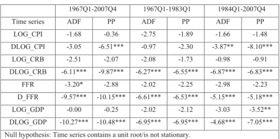
As the visual impression and the description of the data suggest, most of the time series con-tained in the following econometric analysis tend to have a unit root as they exhibit a clear trend. Our unit root tests confirm this guess. The results are presented in table 1. When look-ing at the time series of the logarithm of the CPI and its first difference, the null hypothesis of a unit root cannot be rejected for the first subsample. This is due to the two oil price shocks of the 1970s. Nevertheless, as the time series is stationary when considering the whole sample,
11
As the unit root tests indicate, the CPI is possibly non-stationary. While this might dilute our results, we ad-dress this issue in our robustness checks.
we regard the CPI as integrated of order one. For the time series of the Federal Funds Rate (FFR), the CRB index (CRB) and the GDP, the evidence is clear – both time series are I(1).
Table 1: Unit root tests
1967Q1-2007Q4 1967Q1-1983Q1 1984Q1-2007Q4
Time series ADF PP ADF PP ADF PP
LOG_CPI -1.68 -0.36 -2.75 -1.89 -1.66 -1.48 DLOG_CPI -3.05 -6.51*** -0.97 -2.30 -3.87** -8.10*** LOG_CRB -2.51 -2.07 -2.08 -1.73 -0.98 -0.91 DLOG_CRB -6.11*** -9.87*** -6.27*** -6.55*** -6.87*** -6.83*** FFR -3.20* -2.88 -2.02 -2.25 -2.98 -2.23 D_FFR -9.57*** -10.15*** -6.61*** -6.53*** -5.15*** -5.18*** LOG_GDP -0.00 -0.25 -2.02 -2.12 -3.03 -3.52** DLOG_GDP -10.27*** -10.48*** -6.95*** -6.95*** -4.68*** -7.05*** Null hypothesis: Time series contains a unit root/is not stationary.
*, **, *** indicate a rejection of the null hypothesis at the 10%-, 5%- and 1%-level.
The test equations include a constant and a linear trend. A “D” at the beginning of the name of a time series means that the test is performed in first differences. Accordingly, “LOG” indi-cates that we use the natural logarithm.
4.3 Commodity prices and inflation – prima facie evidence
Figure 1 displays the CRB Spot Index and annual CPI inflation. The first impression suggests a very close link between the CRB Spot index and the annual inflation rate from the begin-ning of the sample in 1968Q1 up to the beginbegin-ning of the 1980s. Afterwards, it seems that the relationship has somewhat weakened. This impression is supported when taking a look at cor-relation coefficients. Regarding the whole sample, the corcor-relation coefficient is -0.08. For the period from 1968Q1 to 1982Q4, the strong co-movement finds evidence in a correlation coef-ficient of 0.81. Afterwards, only weak correlations of about less than 0.25 are detected. This finding supports the assumption that there is a connection between commodity prices and in-flation. Nevertheless, it does not indicate a lead of commodity prices ahead of inin-flation. In fact, it corroborates the view that the connection has weakened during the last decades. Figure 2 displays the annual change of the CRB Spot Index and CPI inflation four quarters ahead. We can establish a close connection from the beginning of the period under review to the middle of the 1980s. From the beginning of the 1990s, the relation somewhat deteriorates.
Figure 1: CRB Spot Index and CPI inflation 0 2 4 6 8 10 12 14 16 0 50 100 150 200 250 300 350 400 450 1968/Q1 1973/Q1 1978/Q1 1983/Q1 1988/Q1 1993/Q1 1998/Q1 2003/Q1
CRB Spot Index CPI inflation in % (rhs)
However, there seems to be a reinforcement starting at the beginning of the new millennium, whereas the lead of the CRB index might have grown a little. Correlation coefficients support this notion. Regarding the whole sample, yields a correlation coefficient of 0.49, which is strong compared to the small negative correlation of the level of the CRB index and CPI infla-tion. Considering the period 1968Q1 to 1983Q4, there is even a stronger co-movement indi-cated by a correlation coefficient of 0.62. When taking a look at the observations from 2000Q1 to 2007Q4 we find the strongest correlation amounting to 0.61 at a lead of the CRB index of seven quarters.
Figure 2: CRB Spot Index and CPI inflation four quarters ahead
0 2 4 6 8 10 12 14 -30 -20 -10 0 10 20 30 40 50 60 70 1968/Q1 1973/Q1 1978/Q1 1983/Q1 1988/Q1 1993/Q1 1998/Q1 2003/Q1 CRB Spot Index, annual change in % annual CPI inflation in %, 4 quarters ahead (rhs)
4.4 Granger causality tests
At first we will take a look at the CRB Spot Index and the CPI (table 2). Granger causality tests are carried out for different lag lengths for the whole sample, as well as for the two sub-samples. To avoid problems of Granger causality tests with non-stationary time series, all tests are performed in first differences.12
Table 2: Granger causality tests (CPI and CRB index)
Lags 67Q1-07Q4 67Q1-83Q1 84Q1-07Q4 67Q1-07Q4 67Q1-83Q1 84Q1-07Q4 1 1.919 3.309* 0.276 3.924** 9.982*** 2.736 2 2.167 5.953*** 1.368 1.679 6.141*** 2.329 3 1.892 3.948** 1.152 3.423** 5.940*** 2.341* 4 1.612 3.261** 0.901 3.593*** 7.534*** 2.084* 5 1.176 1.873 0.701 3.035** 5.505*** 1.644 6 1.059 1.658 0964 3.058*** 3.747*** 2.367**
Null: D_CPI does not Granger-cause D_CRB Null: D_CRB does not Granger-cause D_CPI *, **, *** indicate a rejection of the null at the 10%-, 5%- and 1%-level
Considering the whole sample, we have strong evidence that there is causation only in one direction. While there is no significant causation from the CPI to the CRB index, we find sig-nificant causality at five of six lag lengths for the other direction. This supports our overall working hypothesis that commodity prices might be informative when thinking about future inflation. Furthermore, the analysis of the parted sample backs our visual impression that there might be a weaker link between commodity prices and the CPI today than 25 years ago. While we have significant two-way causation in the earlier period, there is only little evidence of causation from the CRB to the CPI in the period 1984Q1-2007Q4.
In a next step, we take a look at the CRB index and CPI inflation. The results are shown in table 3. Here our assumptions gain further support. While there is no causality from CPI infla-tion to the CRB at no lag in no sample, the picture is completely the opposite when taking a look at Granger-causation from the CRB index to CPI inflation. For the whole sample as well as for the first subsample, the null hypothesis of no causation from the CRB index to CPI in-flation is rejected with a level of significance of 1%. For the sample 1984Q1 to 2007Q4 there
is only little indication of causation which supports our notion of a decreasing relationship between commodity prices and prices of consumer goods.
Table 3: Granger causality tests (CPI inflation and CRB index)
Lags 67Q1-07Q4 67Q1-83Q1 84Q1-07Q4 67Q1-07Q4 67Q1-83Q1 84Q1-07Q4 1 0.154 1.125 0.003 17.321*** 14.973*** 2.650 2 0.131 0.740 1.994 9.378*** 8.350*** 3.123** 3 0.454 0.150 1.860 7.680*** 9.584*** 2.416* 4 0.671 0.962 1.755 5.222*** 8.751*** 0.926 5 0.325 1.106 1.451 4.826*** 7.276*** 0.775 6 0.258 1.084 1.588 3.943*** 5.476*** 0.986
Null: D_INFL does not Granger-cause D_CRB Null: D_CRB does not Granger-cause D_INFL *, **, *** indicate a rejection of the null at the 10%-, 5%- and 1%-level
Table 4: Granger causality tests (CPI inflation and annual change of CRB index) Lags 67Q1-07Q4 67Q1-83Q1 84Q1-07Q4 67Q1-07Q4 67Q1-83Q1 84Q1-07Q4 1 0.034 0.308 1.578 25.233*** 20.354*** 2.173 2 0.059 0.837 2.904* 15.804*** 12.604*** 2.641* 3 0.498 1.584 2.568* 11.373*** 8.566*** 2.161* 4 0.361 0.710 2.201* 6.644*** 5.278*** 2.499** 5 0.412 0.590 2.287* 5.592*** 4.460*** 2.024* 6 0.414 0.448 1.210 5.770*** 4.026*** 1.666
Null: D_INFL does not Granger-cause CRB_GR Null: CRB_GR does not Granger-cause D_INFL *, **, *** indicate a rejection of the null at the 10%-, 5%- and 1%-level
Finally, we investigate whether there is Granger causality when considering annual changes for the CRB index and CPI inflation.13 Table 4 displays the outcomes. When taking a look at the whole sample from 1967Q1 to 2007Q4 and the subsample from 1967Q1 to 1983Q1 we find strict causation from commodity prices to consumer goods inflation. All entries in col-umns five and six of table 4 are significant at the 1%-level, whereas there is no significant entry in columns two and three. Considering our second subsample, we find two-way causa-tion, which seems to be robust to the choice of the lag length but the significance is somewhat weaker. This finding supports the impression from figure 2. There, we had indications of a
13
As unit root tests indicate (not shown here), the annual change of the CRB is already stationary, so we do not have to take first differences.
revival of the connection between CPI inflation and the CRB growth rate starting around the year 2000.
To sum up the results of our battery of Granger causality tests, we conclude that the prima facie evidence seems to give a good indication of what the relationship between commodity prices and consumer goods prices might be like. Furthermore, the economic theory presented in section two appears to be correct, as it delivers plausible arguments for a reduction of the link between commodity prices and the CPI.
4.5 Methodology
In the following we make use of so called structural or identified vector autoregressive (SVAR) models, which were introduced by Sargent (1979) and Sims (1980). Sims (1980) criticized structural economic models because to him their identification scheme is “incredi-ble”. Large-scale models contain too many restrictions and are often highly overidentified. So he argues that VAR models should be used instead.14
Due to the critique of the classical VAR methodology Sims (1981, 1986), Blanchard and Watson (1984) and Bernanke (1986) introduced a new class of VAR models which is called structural or identified VAR. Identification of the model is reached not by an ad hoc Choleski decomposition but by restrictions for the error terms derived from economic theory. In gen-eral, one imposes just as many restrictions as necessary to just identify the system.
Equation (1) shows a structural economic model with n endogenous variables and a constant. For writing purposes, we take up just one lag.15 Furthermore, we assume that the structural innovations are uncorrelated as it is done for example by Sims and Zha (1998).
¸¸ ¸ ¸ ¸ ¹ · ¨¨ ¨ ¨ ¨ © § ¸¸ ¸ ¸ ¸ ¹ · ¨¨ ¨ ¨ ¨ © § ¸¸ ¸ ¸ ¸ ¹ · ¨¨ ¨ ¨ ¨ © § ¸¸ ¸ ¸ ¸ ¹ · ¨¨ ¨ ¨ ¨ © § ¸¸ ¸ ¸ ¸ ¹ · ¨¨ ¨ ¨ ¨ © § ¸¸ ¸ ¸ ¸ ¹ · ¨¨ ¨ ¨ ¨ © § nt t t t n t t nn n n n n n nt t t n n n n e e e y y y a a a a a a a a a a a a y y y b b b b b b ... ... ... ... ... ... ... ... ... ... ... 1 ... ... ... ... ... ... 1 ... 1 2 1 1 , 1 , 2 1 , 1 2 1 2 22 21 1 12 11 0 20 10 2 1 2 1 2 21 1 12 t t t A A y e y B 0 1 1 (1)
14 Although VAR models are frequently used in econometrics, there is also some critique. See, for instance Coo-ley and LeRoy (1985).
15
To find out the appropriate lag length of the system one can use information criteria such as the Akaike or Schwarz criterion.
By premultiplying both sides of equation (1) with the inverse of B denoted as B1 one gets
the reduced form of (1):
t t t B A B A y B e y B B 1 1 1 1 0 1 1 t t t y u y 3 3 0 1 1 , (2) where 0 1 0 B A 3 , 1 1 1 B A 3 and t t B e u 1 .
The structural shocks et can be computed from the reduced form error terms ut by et But (equation (3)). To identify the model, it is necessary to impose some restrictions on the
pa-rameter matrix B. When there are n variables in the system, one has to implement 2
) 1 (n
n
restrictions on the matrixB. So for a four variable VAR, six restrictions must be found to just identify the system.
(3)
Starting with the first equation, we restrict b13 and b14 to zero (Sims and Zha, 1998). This implies that monetary policy cannot respond contemporaneously to developments in con-sumer prices and output due to lags in statistical publications. We do not restrict b12 because data for commodity prices are available daily and so it is possible for central bankers to in-clude commodity price developments in their decision making. Turning to the commodity price equation, we do not restrict any coefficient to zero. We justify this by the fact that com-modity prices are forward-looking and will probably respond to new information quite fast. In line three of matrix B, we restrict b31,b32 and b34 to zero. We do this because we assume that the consumer price level is predetermined (McCoy, 1997). Consumer prices will not react immediately to changes in economic activity, commodity prices or monetary policy. The slower reaction of consumer prices in comparison with commodity prices can be advocated with the economic theory of section two as well. Finally, we impose the restriction b41 0. By doing this we assume that the output reacts to changes in monetary policy only with a lag (Bernanke and Blinder, 1992).
¸ ¸ ¸ ¸ ¸ ¹ · ¨ ¨ ¨ ¨ ¨ © § ¸¸ ¸ ¸ ¸ ¹ · ¨¨ ¨ ¨ ¨ © § ¸ ¸ ¸ ¸ ¸ ¹ · ¨ ¨ ¨ ¨ ¨ © § GDP t CPI t CRB t FFR t GDP t CPI t CRB t FFR t u u u u b b b b b b b b b b b b e e e e 1 1 1 1 43 42 41 34 32 31 24 23 21 14 13 12
4.6 Results
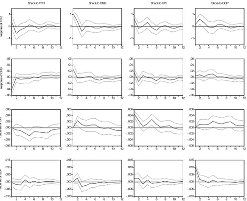
Figure 3 and 4 show the impulse response functions for the two subsamples of our baseline model with 95% error bands. Each row mirrors the reaction of one variable to the four differ-ent shocks. Accordingly, each column shows the reaction of the variables to one specific shock. In reference to the scope of this paper, we are mainly interested in the impulse re-sponses in the first column, as we can find there the reaction of the variables to a monetary policy shock. Beyond this, the impulse response of the CPI to a CRB shock and vice versa is of special interest.
Figure 3: Impulse responses, 1967Q1-1983Q1, baseline model
-1 0 1 2 4 6 8 10 12 Shock to FFR -1 0 1 2 4 6 8 10 12 Shock to CRB -1 0 1 2 4 6 8 10 12 Shock to CPI -1 0 1 2 4 6 8 10 12 Shock to GDP -.06 -.04 -.02 .00 .02 .04 .06 2 4 6 8 10 12 -.06 -.04 -.02 .00 .02 .04 .06 2 4 6 8 10 12 -.06 -.04 -.02 .00 .02 .04 .06 2 4 6 8 10 12 -.06 -.04 -.02 .00 .02 .04 .06 2 4 6 8 10 12 -.006 -.004 -.002 .000 .002 .004 .006 2 4 6 8 10 12 -.006 -.004 -.002 .000 .002 .004 .006 2 4 6 8 10 12-.006 -.004 -.002 .000 .002 .004 .006 2 4 6 8 10 12-.006 -.004 -.002 .000 .002 .004 .006 2 4 6 8 10 12 -.010 -.005 .000 .005 .010 .015 2 4 6 8 10 12 -.010 -.005 .000 .005 .010 .015 2 4 6 8 10 12-.010 -.005 .000 .005 .010 .015 2 4 6 8 10 12-.010 -.005 .000 .005 .010 .015 2 4 6 8 10 12 re spons e of F FR re spons e of C R B re sp on se o f C P I re spons e of G D P
Regarding figure 3, showing the results for the 1967Q1-1983Q3 sample, we detect a reduction of commodity prices and consumer prices after a restrictive monetary policy, i.e. a raise of the Federal Funds Rate. Commodity prices decrease immediately (and significantly), consumer prices decline significantly not until one year. This fits our hypothesis of a fast reaction of commodity prices in comparison to consumer prices quite well. As commodity prices react
instantaneously, we can explain the finding of a reduction in interest rates after a tightening of monetary policy. The monetary authority gets the feedback by the reaction of commodity prices that the means applied are working and therefore monetary policy returns to the previ-ous path of a less tight policy indicated by a reduction of the Federal Funds Rate.16 Further-more, the response pattern of the CPI is what is usually expected when thinking about mone-tary policy transmission. A more restrictive monemone-tary policy should decrease the price level. For the period 1967Q1-1983Q1 we cannot identify a “price puzzle”, which is a rise of con-sumer prices after a more restrictive monetary policy. This makes us confident that we have identified monetary policy correctly (Hanson, 2004).
Another interesting result emerges when taking a look at the reaction of the CPI to a structural CRB shock and vice versa. We identify an immediate and significant rise of consumer prices to an exogenous increase of the CRB index. Thus, commodity prices influence the evolution of the CPI. When we regard the reaction of commodity prices to an increase in consumer prices we detect only an insignificant albeit rectified reaction. This somewhat reflects the Granger causality tests for the first subsample presented in table 2.
In addition we can find a significant rise in interest rates both for a commodity price shock and a CPI shock. This underlines the connection between monetary policy, commodity prices and inflation as well.
Taking now a look at the other impulse response functions, we detect an anticyclical monetary policy. We see that a demand shock, i.e. an unanticipated rise in the GDP growth rate, leads to a significant rise in interest rates. This is what one would expect because central bankers and especially the Fed have to take a look at the economic performance as well. Considering the other impulse response functions we find no significant change in the GDP growth rate to shocks in both the consumer and commodity price level. Beyond this we see a significant rise in the consumer price level after an increase in the GDP. This can be explained by rising de-mand which fuels inflationary pressure.
Focussing now on figure 4, displaying the results for the period 1984Q1-2007Q4, the first impression we get is that we have far less significant reactions than in the first sample. This finding is corroborated by Herrera and Pesavento (2009). We take this as a sign of a decreas-ing relationship between commodity prices and the overall economic situation. Considerdecreas-ing the reaction of the two price indices to a monetary policy shock we do not find any significant
16
These findings allow the statement that for the first subsample commodity prices might not have been only an indicator variable for central bankers but an intermediate target as well.
response neither of the CRB nor of the CPI. At least the tendency of the response functions is correct and the time path fits the story of a quicker reaction of commodity prices. Additionally, we do not find a price puzzle. As we cannot detect any significant response of the CRB index to monetary policy, the CRB index cannot be seen as an intermediate target.
Figure 4: Impulse responses, 1984Q1-2007Q4, baseline model
-.2 .0 .2 .4 .6 2 4 6 8 10 12 Shock to FFR -.2 .0 .2 .4 .6 2 4 6 8 10 12 Shock to CRB -.2 .0 .2 .4 .6 2 4 6 8 10 12 Shock to CPI -.2 .0 .2 .4 .6 2 4 6 8 10 12 Shock to GDP -.06 -.04 -.02 .00 .02 .04 2 4 6 8 10 12 -.06 -.04 -.02 .00 .02 .04 2 4 6 8 10 12 -.06 -.04 -.02 .00 .02 .04 2 4 6 8 10 12 -.06 -.04 -.02 .00 .02 .04 2 4 6 8 10 12 -.002 .000 .002 .004 .006 2 4 6 8 10 12 -.002 .000 .002 .004 .006 2 4 6 8 10 12-.002 .000 .002 .004 .006 2 4 6 8 10 12-.002 .000 .002 .004 .006 2 4 6 8 10 12 -.004 -.002 .000 .002 .004 .006 2 4 6 8 10 12 -.004 -.002 .000 .002 .004 .006 2 4 6 8 10 12-.004 -.002 .000 .002 .004 .006 2 4 6 8 10 12-.004 -.002 .000 .002 .004 .006 2 4 6 8 10 12 re spons e of F FR re spons e of C R B re spon se of C PI re spons e of G D P
For the response of consumer prices to a CRB shock, we do not find a significant reaction. This is documented by Furlong and Ingenito (1996) as well. They use a bivariate VAR of consumer and commodity prices. Their split sample analysis with a structural break at the end of 1983 exhibits a response pattern similar to ours. While the CPI rises significantly after a shock to the CRB index considering the period from1973M01-1983M12, they do not find such a reaction when looking at the period from 1984M01-1995M11.
The same holds true for the reaction of the CRB index to an unanticipated rise in the CPI growth rate. We cannot detect a significant response. Thus our hypothesis of a decreasing or even disappearing relationship gains support from these impulse response functions.
Consid-ering the other impulse response functions we again find an anticyclical monetary policy indi-cated by a rise in interest rates to an increase in the GDP growth rate.
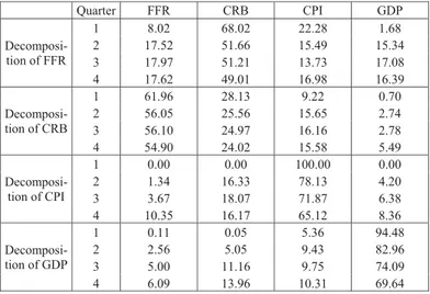
In a next step we will take a look at variance decompositions to find additional support for our hypothesis. Variance decompositions allow us to distinguish whether commodity price swings are important in explaining changes in consumer prices. Table 5 and 6 display the variance decompositions for the two subsamples.
Table 5: Variance decompositions, 1967Q1-1983Q1, baseline model
Quarter FFR CRB CPI GDP Decomposi-tion of FFR 1 8.02 68.02 22.28 1.68 2 17.52 51.66 15.49 15.34 3 17.97 51.21 13.73 17.08 4 17.62 49.01 16.98 16.39 Decomposi-tion of CRB 1 61.96 28.13 9.22 0.70 2 56.05 25.56 15.65 2.74 3 56.10 24.97 16.16 2.78 4 54.90 24.02 15.58 5.49 Decomposi-tion of CPI 1 0.00 0.00 100.00 0.00 2 1.34 16.33 78.13 4.20 3 3.67 18.07 71.87 6.38 4 10.35 16.17 65.12 8.36 Decomposi-tion of GDP 1 0.11 0.05 5.36 94.48 2 2.56 5.05 9.43 82.96 3 5.00 11.16 9.75 74.09 4 6.09 13.96 10.31 69.64
Table 5 gives the results for the 1967Q1-1983Q1 sample. Starting with the variance decom-position of the change of the Federal Funds Rate we find that it is primarily the CRB index which explains the variation of monetary policy. About one half of the variation in the Federal Funds Rate is due to changes in commodity prices. This is somewhat surprising as the Fed is concerned about consumer price stability rather than commodity prices. However, remember-ing the economic theory and the empirical evidence up to now, we know that commodity prices can serve as indicator variables for monetary policy. Additionally, we should keep in mind that monetary policy is likely to react to macroeconomic conditions. Variations in the Federal Funds Rate should be explained by macroeconomic variables as can be seen here. Turning to the CRB decomposition in table 5 we see that monetary policy has got strong in-fluences on commodity prices as well. Variation in commodity prices is explained to around 55% by changes in interest rates. These outcomes underline once more that there is a strong
link between monetary policy and commodity prices in the time of the first two oil price shocks.
For consumer prices, shocks of the CRB index, the GDP or the interest rate have got similar magnitudes of about 10%-15%. A comparable result is presented by Garner (1989). In his model commodity prices account for one fourth of the variation in the CPI. Regarding GDP, it is its own shock that dominates its variance. All other shocks account each for about 10% of the variance in output.
The variance decompositions for the 1984Q1-2007Q4 sample are shown in table 6. We can verify our guess of a lower influence of commodity prices for monetary policy. Changes in commodity prices no longer dominate the evolution of the Federal Funds Rate. Although variations in the CRB index account for about 30% of the variance in interest rates, this is a clear reduction compared to the 55% in the 1967Q1-1983Q1 sample. Hence, we can conclude that monetary policy has responded less to commodity price developments, probably knowing that the quality of the signals sent by commodity prices has deteriorated. The influence of changes in output has increased. One explanation of this finding might be that in the course of the Great Moderation central bankers could focus more and more on smoothing the business cycle and supporting the economic activity than fighting inflation. This argument is somewhat sustained by the reduced influence of changes in consumer prices for monetary policy changes. Nevertheless, macroeconomic conditions still account for a large part of the varia-tion in the Federal Funds Rate.
Moving on to the variance decomposition of the rate of change of the CRB index, we see that monetary policy changes account for far less variation than in the first subsample. This allows the conclusion that monetary policy is no longer able to influence commodity prices and that the overall link between monetary policy and commodity prices has decreased.
The last two variance decompositions shown in table 6, exhibit the same pattern. For both, it is about 90% the own shock that accounts for variations in the time series. All other factors are negligible. For the CPI the influence of commodity prices decreased. While changes in the CRB index account for about 15% of the variation in the CPI in the early sample, the influ-ence of the CRB index sinks to less than 5%. This finding is corroborated by Furlong and Ingenito (1996). Their variance decompositions for bivariate VAR models exhibit the same pattern. For the more recent sample the CRB index accounts for only 11% in the variation of the CPI, while it was about 30% considering the earlier sample.
Table 6: Variance decompositions, 1984Q1-2007Q4, baseline model Quarter FFR CRB CPI GDP Decomposi-tion of FFR 1 55.87 36.80 2.10 5.22 2 42.54 33.02 2.97 21.46 3 39.95 29.53 3.69 26.83 4 39.06 28.56 5.24 27.14 Decomposi-tion of CRB 1 23.35 63.93 3.65 9.07 2 21.86 60.47 3.67 14.00 3 20.72 60.06 6.02 13.20 4 20.31 60.93 6.05 12.71 Decomposi-tion of CPI 1 0.00 0.00 100.00 0.00 2 0.13 1.75 97.49 0.62 3 2.23 1.82 90.84 5.11 4 2.78 2.55 89.78 4.89 Decomposi-tion of GDP 1 0.58 1.58 1.72 96.13 2 1.23 3.95 1.57 93.25 3 1.69 3.60 1.90 92.81 4 1.69 6.53 2.40 89.39
Summarising the results from the variance decompositions, we can say that the findings con-firm the results presented in the impulse response analysis. The connection between monetary policy, commodity prices and inflation is weaker than it was in the period before the 1980s. This notion is held by Blanchard and Galí (2008) as well. Although they focus on oil price shocks and their relation to the overall economic performance, they report a shrinking influ-ence of oil price movements on prices. Another study that corroborates our results is that of Furlong and Ingenito (1996). They take a look at bivariate VAR models for commodity prices and inflation. They use rolling regressions as well as VAR models for subperiods and con-clude that commodity prices were reliable indicators for CPI inflation in the 1970s up to the beginning of the 1980s. Afterwards, the performance of commodity prices as a leading indica-tor of consumer prices considerably deteriorates. A comparable approach is found in De Gregorio et al. (2007). They use rolling regressions with a length of 200 months and investi-gate the pass-through of oil prices to consumer prices for various countries. They find a de-clining pass-through of oil prices to the general price level. However, for the US they detect reinforcement in the recent years.17 Herrera and Pesavento (2009) document similar results as ours. Although they focus on the effect of oil price shocks, their approach has various inter-sections with ours: they use quarterly data, incorporate four lags in their VAR model and split their sample in the middle of the 1980s. Their findings of a decreased influence of oil price shocks on prices in the second subperiod strongly resemble our results.
4.7 Robustness checks
Although our baseline model seems to be well specified when regarding the diagnostic tools, there might be problems due to the fact that the time series of the CPI is likely to be non-stationary in our first sample. Hence, it is advisable to check the results from our model and perform some robustness checks.
First, we replace the time series of the CPI in our VAR model by the annual inflation rate. Because for the inflation rate, the results of unit root tests are mixed, we include the inflation rate in first differences. Model diagnostic tests exhibit similar results like the baseline model. Regarding the impulse response functions, we get nearly the same results with only slight differences for both samples.18 For the first period we now find a significant reduction in the growth rate of the GDP in response to a tightening of monetary policy. This reduction takes place after three quarters and so two quarters before the consumer prices level significantly shrinks. So this modification fits better the generally accepted timing of the monetary trans-mission process. Apart from that we cannot find any striking differences, in fact, the response patterns seem to be duplicates of the ones from our baseline model. The same holds true for the second sample. The only difference we detect is a significant rise of the Federal Funds Rate after an unexpected increase in the commodity price index. However, this is due to smaller error bands at the beginning in comparison with the impulse response function re-ceived from the baseline specification. The response patterns in both cases are almost the same. Variance decompositions support the finding of no dramatic change. For the first period, we detect a less strong influence of monetary policy in determining the evolution of the CRB index. For the 1984Q1-2007Q4 sample we cannot find any eye-catching differences at all. In a next step we replace the GDP by the index of industrial production (the CPI has returned to our model). The use of the industrial production can be justified by the fact that commodi-ties are used especially in the manufacturing sector and not in the service sector. So the index of industrial production might be a more appropriate activity measure than the GDP because the GDP consists largely of services which are independent of commodity price changes. Again we find no evidence of severe misspecification and the impulse response functions for the first period show the same pattern. We just detect a stronger rise in the consumer price level after an increase in industrial production. Variance decompositions corroborate the re-sults from the baseline model, too. The impulse response functions and the variance decom-positions derived for the second period strongly resemble the results from the baseline model.
18
The figures are not shown here because they exhibit no dramatic changes. However, they are available upon request.
Solely the variance decompositions of the change in the Federal Funds Rate and the growth rate of the CRB index do differ from the results obtained by the baseline model. Movements of commodity prices and consumer prices account for about 70% of the variations in mone-tary policy. The Federal Funds Rate’s own shock is not the main influence as it is in the base-line model. For the variance decomposition of the rate of change of the CRB index we find that the Federal Funds Rate, the CPI and the index of industrial production account for a lar-ger part of the variation than it was the case in the baseline model. The CRB’s own influence sinks from 60% to 45%.
Finally, we replace the broad commodity price index by the CRB Raw Industrials Sub-index (in log differences), but once more there are no large differences in impulse response func-tions. We should only mention the finding that for the period 1984Q1 to 2007Q4 the CRB Raw Industrials Sub-index accounts for about 60% of the variance of the changes in interest rates and monetary policy is responsible for almost 60% of the variance in the CRB sub-index. This is somehow against the results we have presented till now because it suggests that there still might be a link between monetary policy and commodity prices. Thus, further research could be addressed this issue, whether there are narrow commodity prices aggregates or spe-cial commodity prices such as gold which can serve as indicator variables for monetary policy today.
Our next step in robustness analysis is to change the identification pattern of the VAR model. For simplicity we will perform these checks only for the baseline model. At first, we allow a contemporaneous reaction of monetary policy to output and consumer prices, i.e. we do no longer restrict b13 and b14 in the matrix in equation (3) to zero. We do this because central bankers might have indicator variables they consider when taking policy decisions. In return we restrict b23 and b42 to zero. We justify this with the thought of delivery contracts that pre-serve enterprises to react immediately to changes in production when commodity prices alter. While most of the impulse response functions do not change a lot, the price puzzle occurs when considering the first subsample. We take this as an indication of misspecification and do not go into detail concerning the impulse response functions and variance decompositions. Alternatively, we try several Choleski orderings as proposed by Sims (1986). For the ar-rangement of the variables we follow the advice of Favero (2001) to put monetary variables last because they are supposed to react faster than other variables. The first ordering we test is output, consumer prices, commodity prices and interest rates. The impulse response functions exhibit several differences. Neither for the first nor for the second sample, we detect a
signifi-cant response of the CRB index to a tightening of monetary policy. For the first period under review, we even find a small increase in consumer prices in response to a more restrictive monetary policy. Nevertheless, at least the response pattern with a reduction after several quarters fits economic theory (although the response is not significant). The variance decom-positions now exhibit that most of the variation in a variable is explained by its own shock. This holds true especially for the second sample under review.
Changing the CRB index and the Federal Funds Rate in the Choleski ordering yields even a more explicit price puzzle and we cannot find a significant response of commodity prices to a rise in the Federal Funds Rate in the first sample but besides this, there are no substantial changes. What we mentioned for the variance decompositions with the first Choleski ordering applies here as well.
5. Conclusion and policy implications
The past years were characterized by unprecedented rises in prices of commodities such as oil or wheat and inflation rates moved up above the mark of two percent per annum which is typically referred to as price stability. This led to a debate whether commodity prices indicate future CPI inflation and if they can be used as indicator variables for central banks.
To answer this question, we have investigated what the connection between commodity prices and inflation is like in the US. After having looked at the economic theory which delivers reasons for and against a relationship between prices of both sorts of goods, we applied vari-ous econometric methods like Granger causality tests and SVAR models to answer this ques-tion.
All these tools pointed to one conclusion. While there was a strong link between commodity prices and CPI inflation in the 1970s and the beginning of the 1980s, the relationship has weakened, respectively diminished over time. Today we are unable to detect a reaction of commodity prices to commodity price shocks. Thus, commodity prices might not serve as good indicator variables for monetary policy. Our results are pretty in line with the findings of Furlong and Ingenito (1996), De Gregorio et al. (2007) and Herrera and Pesavento (2009). In all these papers a reduced relationship between commodity prices and inflation is documented. One starting point for further analyses is to enlarge the VAR model to be able to distinguish which factor named in the second section is responsible for the weakening of the relationship between commodity prices and inflation. Another promising approach might be to investigate
whether there is a revival of the link in the last few years. De Gregorio et al. (2007) hint at this and we have found little evidence of reinforcement as well. However, right now this is somewhat difficult to investigate with econometric methods because of few observations, especially when using quarterly data. Moreover, Krichene (2008) speculates if it is simply too early to detect such a recovery because of the monetary transmission mechanism which may take some more time.
Regarding our results, we would not use commodity prices as an indicator variable for mone-tary policy. At the moment, policymakers should not take commodity price changes as signals for future CPI inflation. As seen, the rise of commodity prices was merely temporary and we have noticed a sharp drop after the records reached in 2007 and 2008. Thus, these swings in commodity markets reflect probably to a large extent speculative behaviour of investors. The ample and cheap liquidity available on international financial markets searches for yield and as interest rates are quite low, commodities might be a worthwhile alternative for investments. Furthermore, a more restrictive monetary policy in face of rising commodity prices could de-press economic activity. This is problematic especially for the Fed as she has to focus on price stability and the support of the economic performance of the American economy. Regarding the actual financial crisis, putting more weight on stimulating the economic activity might be superior to eliminate inflationary pressure. Additionally, higher inflation rates as a conse-quence of the fairly expansionary monetary policy would come along with a (to some minds) nice side effect of devaluating the governmental debt. Therefore, keeping interest rates low might lead to a reduction of the deficit relative to GDP for two reasons: higher growth rates decrease debt relative to GDP and inflation erodes the real value of the debt.
Nevertheless, central banks should monitor if commodity prices will influence inflation ex-pectations. As food and petrol are goods which are bought quite frequently, a rise in these commodity prices can increase inflation expectations, with the risk of a stronger influence of commodity prices on the CPI in the future. So the hypothesis of a revival is not so far off which points to no quietening of the discussion about commodity prices, monetary policy and inflation.
References
Adams, F. G., Ichino, Y. (1995): Commodity Prices and Inflation: A Forward-Looking Price Model, Journal of Policy Modeling, Vol. 17, No. 4, pp. 397-426.
Alchian, A. A., Klein, B. (1973): On a Correct Measure of Inflation, Journal of Money, Credit and Banking, Vol. 5, No. 1, February, pp. 173-191.
Angell, W. D. (1992): Commodity Prices and Monetary Policy: What Have We Learned?, Cato Journal, Vol. 12, No. 1, Spring/Summer, pp. 185-192.
Awokuse, T. O., Yang, J. (2003): The Informational Role of Commodity Prices in Formulat-ing Monetary Policy: A Reexamination, Economic Letters, Vol. 79, No. 2, May, pp. 219-224.
Barnhart, S. W. (1989): The Effect of Macroeconomic Announcements on Commodity Prices, American Journal of Agricultural Economics, Vol. 71, No. 2, May, pp. 389-403.
Barsky, R. B, Kilian, L. (2002): Do We Really Know that Oil Caused the Great Stagflation? A Monetary Alternative, NBER Macroeconomic Annual, May, pp. 137-183.
Belke, A., Bordon, I. G., Hendricks, T. W. (2009): Global Liquidity and Commodity Prices – A Cointegrated VAR Approach for OECD Countries, Ruhr Economic Papers, No. 102. Belongia, M. T. (1991): Monetary Policy and the Farm/Nonfarm Price Ratio: A Comparison
of Effects in Alternative Models, Federal Reserve Bank of St. Louis Review, Vol. 73, No. 4, July/August, pp. 30-46.
Bermingham, C. (2008): Quantifying the Impact of Oil Prices on Inflation, Research Techni-cal Paper 8/08, November, Economic Analysis and Research Department, Central Bank and Financial Services Authority of Ireland.
Bernanke, B. S. (1986): Alternative Explanations of the Money-Income Correlation, NBER Working Paper No. 1842, February.
Bernanke, B. S., Blinder, A. S. (1992): The Federal Funds Rate and the Channels of Monetary Transmission, American Economic Review, Vol. 82, No. 4, September, pp. 901-921. Bhar, Ramaprasad, Hamori, Shigeyuki (2008): Information Content of Commodity Future
Prices for Monetary Policy, Economic Modelling, Vol. 25, No. 2, pp. 274-283.
Blanchard, O. J., Watson, M. W. (1984): Are Business Cycles All Alike?, NBER Working Paper No. 1392, June.
Blanchard, O. J., Galí, J. (2008): The Macroeconomic Effects of Oil Price Shocks: Why are the 2000s so different from the 1970s?, CEPR Discussion Paper No. 6631.
Blomberg, S. B., Harris, E. S. (1995): The Commodity-Consumer Price Connection: Fact of Fable?, Federal Reserve Bank of New York Policy Review, October, pp. 21-38.
Bordo, M. D. (1980): The Effects of Monetary Change on Relative Commodity Prices and the Role of Long-Term Contracts, Journal of Political Economy, Vol. 88, No. 6, December, pp.1088-1109.
Borio, C., Filardo, A. (2007): Globalisation and Inflation: New Cross-country Evidence on the Global Determinants of Domestic Inflation, BIS Working Paper No. 227, May.
Boughton, J. M., Branson, W. H., Muttardy, A. (1989): Commodity Prices and Inflation: Evi-dence from Seven Large Industrial Countries, IMF Working Paper 89/72, September. Browne, F., Cronin, D. (2007): Commodity Prices, Money and Inflation, ECB Working Paper
No. 738, December.
Cecchetti, S. G., Moessner, R. (2008): Commodity Prices and Inflation Dynamics, BIS Quar-terly Review, December, pp. 55-66.
Cheung, C. (2009): Are Commodity Prices Useful Indicators of Inflation?, Bank of Canada Discussion Paper 2009-5.
Cody, B. J., Mills, L. O. (1991): The Role of Commodity Prices in Formulating Monetary Policy, The Review of Economics and Statistics, Vol. 73, No. 2, May, pp. 358-365.
Cooley, T. F., LeRoy, S. F. (1985): Atheoretical Macroeconometrics: A Critique, Journal of Monetary Economics, Vol. 16, No. 3, November, pp. 283-308.
De Gregorio, J., Landerretche, O., Neilson, C. (2007): Another Pass-Through Bites the Dust? Oil Prices and Inflation, Central Bank of Chile Working Papers, No. 417, May.
Devadoss, S., Meyers, W. H. (1987): Relative Prices and Money: Further Results for the United States, American Journal of Agricultural Economics, Vol. 69, No. 4, November, pp. 838-842.
Dornbusch, R. (1976): Expectations and Exchange Rate Dynamics, Journal of Political Econ-omy, Vol. 84, No. 6, pp. 1161-1176.
European Central Bank (2010): Oil Prices – Their Determinants and Impact on Euro Area Inflation and the Macroeconomy, Monthly Bulletin August, pp. 75-92.
Favero, C. A. (2001): Applied Macroeconometrics, Oxford University Press, New York. Filardo, A. J. (2001): Should Monetary Policy Respond to Asset Price Bubbles? Some
Ex-perimental Results, Federal Reserve Bank of Kansas City Working Paper No. 01-04, July. Frankel, J. A. (1986): Expectations and Commodity Price Dynamics: The Overshooting
Model, American Journal of Agricultural Economics, Vol. 68, No. 2, May, pp. 344-348. Furlong, F. T. (1989): Commodity Prices as a Guide for Monetary Policy, Federal Reserve
Furlong, F. T., Ingenito, R. (1996): Commodity Prices and Inflation, Federal Reserve Bank of San Francisco Economic Review, No. 2, pp. 27-47.
Garner, C. A. (1989): Commodity Prices: Policy Target or Information Variable? A Note, Journal of Money, Credit and Banking, Vol. 21, No. 4, November, pp. 508-514.
Gerlach, S., Smets, F. (1995): The Monetary Transmission Mechanism: Evidence from the G-7 Countries, BIS Working Paper No. 26, April.
Hanson, M. S. (2004): The “Price Puzzle” Reconsidered, Journal of Monetary Economics, Vol. 51, No. 7, October, pp. 1385-1413.
Herrera, A. M., Pesavento, E. (2009): Oil Price Shocks, Systematic Monetary Policy and the “Great Moderation”, Macroeconomic Dynamics, Vol. 13, No. 1, February, pp. 107-137. Hooker, M. A. (2002): Are Oil Shocks Inflationary? Asymmetric and Nonlinear
Specifica-tions versus Changes in Regime, Journal of Money, Credit and Banking, Vol. 34, No. 2, May, pp. 540-561.
Krichene, N. (2008): Recent Inflationary Trends in Commodities Markets, IMF Working Pa-per No. 08/130, May.
Kyrtsou, C., Labys, W. C. (2006): Evidence for Chaotic Dependence between US Inflation and Commodity Prices, Journal of Macroeconomics, Vol. 28, No. 1, pp. 256-266.
LeBlanc, M., Chinn, M. D. (2004): Do High Oil Prices Presage Inflation? The Evidence from G-5 Countries, Santa Cruz Center for International Economics Paper 04/04.
Mahdavi, S., Zhou, S. (1997): Gold and Commodity Prices as Leading Indicators of Inflation: Tests of Long-Run Relationships and Predictive Performance, Journal of Economics and Business, Vol. 49, No. 5, pp. 475-489.
Marquis, M. H., Cunningham, S. R. (1990): Is There a Role for Commodity Prices in the De-sign of Monetary Policy? Some Empirical Evidence, Southern Economic Journal, Vol. 57, No. 2, October, pp. 394-412.
Marschall, B., Beyerle, H. (2009): Spekulanten treiben Ölpreis, in: Financial Times Deutsch-land, 09.06.2009, p. 14.
McConnell, M. M., Perez-Quiros, G. (2000): Output Fluctuations in the United States: What has Changed Since the Early 1980’s?, American Economic Review, Vol. 90, No. 5, Decem-ber, pp. 1464-1476.
McCoy, D. (1997): How Useful is Structural VAR Analysis for Irish Economics?, Economic Analysis, Research and Publication Department of the Central Bank of Ireland, Technical Paper 2/RT/97, April.