Building Software Cost Estimation Models using Homogenous Data

(1)

Building Software Cost Estimation Models using Homogenous Data

Rahul Premraj

· Thomas Zimmermann

Saarland University

Saarbr¨ucken, Germany

{

premraj

· zimmerth

}

@cs.uni-sb.de

Abstract

Several studies have been conducted to determine if company-speciﬁc cost models deliver better prediction ac-curacy than cross-company cost models. However, mixed results have left the question still open for further investiga-tion. We suspect this to be a consequence of heterogenous data used to build cross-company cost models. In this pa-per, we build cross-company cost models using homogenous data by grouping projects by their business sector. Our re-sults suggest that it is worth to train models using only ho-mogenous data rather than all projects available.

1. Introduction

In the last decade, company-speciﬁc cost models have received some attention to determine if they deliver better prediction accuracy than cross-company cost models. Un-fortunately, mixed results from studies conducted to date have left the question still open [9]. In contrast to previous work, in this paper we investigate if cost models built using homogenous cross-company project data (i.e., grouped by business sectors) can yield improved prediction accuracy.

Software cost estimation is inherently a challenging task. This is due to numerous factors such as lack of understand-ing of software processes and their impact on project sched-ule, constantly changing technologies, and the human fac-tor, which adds substantial variability in productivity. Thus, despite over four decades of on-going research, we con-tinue to witness novel approaches being presented to im-prove cost estimation accuracy.

One such proposed approach by Maxwell et al. [12] was to build company-speciﬁc cost models using data originat-ing from a soriginat-ingle company. Such data is likely to be more homogenous and reﬂect the company’s strengths and weak-nesses, and in turn, lead to better models. Thereafter, sev-eral follow-up studies and replications (discussed in Sec-tion 2) were conducted to verify, if indeed, models based on in-house data perform better than those built on data gath-ered across several companies.

Irrespective of the lack of consensus from different studies, a challenging prerequisite for building company-speciﬁc cost models is availability of in-house project data. This might be a constraint for several companies for a vari-ety of reasons such as:

• New companies may be yet to begin implementing projects to extract and record data.

• Recorded data from the past may be irrelevant to esti-mate costs using current technologies.

• Companies may choose not to collect data for they lack incentives to do so.

• Companies may not know what data to collect and how to do so.

What alternatives do such companies have? Clearly, they have to resort to other sources of data to base their own cost estimates on. For this, it is vital that the data originates from comparable companies undertaking similar projects; else the estimates may be considerably off mark. Natural choices in such a scenario are companies from the same business sector. They likely operate within similar environ-ments that expose them to comparable cost factors, and in turn, comparable development productivity [15] and costs.

Using signiﬁcant differences in productivity across busi-ness as a motivation, we seek to verify if building cost models from homogenous companies delivers better results. Within this large goal, the objectives of our study are:

(a) To develop company-speciﬁc cost models for compar-isons against other models[OB1].

(b) To develop cross-company cost models to compare their prediction accuracy against company-speciﬁc cost models[OB2].

(c) To develop business-speciﬁc cost models to compare their prediction accuracy against company-speciﬁc and cross-company cost models[OB3].

(d) To develop business-speciﬁc cost models to determine if they can be used by companies from other business sectors[OB4].

First International Symposium on Empirical Software Engineering and Measurement First International Symposium on Empirical Software Engineering and Measurement

(2)

The road-map of the paper is as follows: Section 2 dis-cusses related work. Next, the data set used for our study is discussed in Section 3. Our design of experiments is pre-sented in Section 4. Sections 5 and 6 present our results from building company-speciﬁc cost models and cross-company cost models respectively using our data (OB1 and OB2). Results from business-speciﬁc cost models (OB3) are presented in Section 7, while results from cross-business cost models (OB4) are reported in Section 8. We discuss threats to validity in Section 9, and conclude in Section 10.

2 Related Work

Several studies have been previously conducted to deter-mine if company-speciﬁc cost models are superior to cross-company cost models in terms of prediction accuracy. Un-fortunately, a systematic review [9] on this topic showed that the results are too mixed to conclude that either of the two models is signiﬁcantly better than the other.

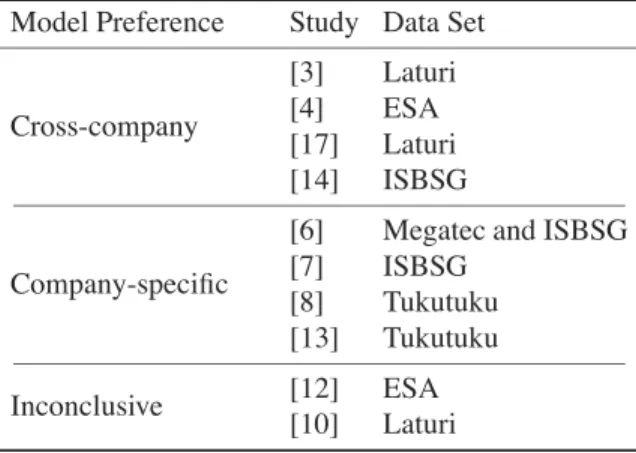
Table 1 presents ten studies dating from 1999 that com-pare cost models across companies. Of these, four studies concluded that company-specific cost models are ‘not’ sig-nificantly better than cross-company cost models. All re-maining six studies concluded the opposite, i.e. company-specific cost models perform better than cross-company models. However, the last two studies in Table 1 ([12, 10]) conducted no statistical significance tests to arrive at their respective conclusions. Hence, in agreement with Kitchen-ham and Mendes [9], we report the two studies as inconclu-sive. Table 1 makes clear the lack of compelling evidence to support claims in favour of either of the two investigated cost models.

The systematic review by Kitchenham and Mendes [9] went further to investigate if quality control for data col-lection could inﬂuence the outcome of the studies. No evi-dence to suggest the same was found. However, a bias was noticed in studies favouring company-speciﬁc cost models since they employed smaller data sets with lower maximum effort values. Also, differences in experimental design and accuracy measures made drawing conclusions in the sys-tematic review challenging.

Clearly, comparable and replicable experiments are re-quired to further investigate the cause for discrepencies in results across different studies. A likely explanation for mixed results is disregarding other factors that inﬂuence development costs. One such factor is the business sector that the company operates in. Premraj et al. [15] showed substantial differences in development productivity across business sectors, where the manufacturing sector was nearly three times more productive than banking and insurance sectors. Hence, it is reasonable to assume that differences in productivity (and those from other factors) may distort cross-company cost models and give overall mixed results.

Table 1. Previous Studies and their Model Preferences (adapted from [9])

Model Preference Study Data Set

Cross-company [3] Laturi [4] ESA [17] Laturi [14] ISBSG Company-speciﬁc

[6] Megatec and ISBSG [7] ISBSG

[8] Tukutuku [13] Tukutuku Inconclusive [12] ESA

[10] Laturi

In contrast to the above studies, we take the business sec-tor explicitly into account in the cost model, motivated by a statistically justiﬁcation [15] for its inclusion, and investi-gate the inﬂuence it casts on prediction accuracy. For this, we use the ‘Finnish Data Set’ that has previously never been used for studies on this subject.

3 The Finnish Data Set

The ‘Experience Pro Data’, commonly referred to as the ‘Finnish Data’, has been used in this study. This section provides a brief background on the data set and furnishes the data cleansing steps undertaken to make it suitable for analysis.

The ‘Finnish Data’ is the result of a commercial initia-tive by Software Technology Transfer Finland (STTF) [1] to support the software industry, especially to benchmark software costs, development productivity and software pro-cesses. So far, constituent projects originate only from Fin-land. To have access to the data, companies are subjected to an annual fee, which may be partially waived in propor-tion to the number of submitted projects by the company. These projects are carefully assessed and graded for quality by experts at STTF, and then committed to the data set.

Since data collection is an on-going process, the data set has been growing over the years. For this study, the version of the data available as of March 2005 is used. We refer to it as Finnish788 since it comprises788projects. The constituent projects span from a wide breadth of business sectors such as banking, insurance, public administration, telecommunications and retail. It includes both, new devel-opment projects (88%) and maintenance projects (remain-ing12%). Other ﬁelds that characterise the projects include effort (in hours), project size (in FiSMA FP), development environment, staff pertaining metrics and many more. In total, over100different variables are collected, but a

(3)

major-ity of them are difﬁcult to analyse given the ratio of missing values. Maxwell and Forselius [11] provide a fuller descrip-tion of the data.

It is obvious that a data set of such scale is bound to have noise that may derive misleading results. To counter this, we removed suspect projects from the data set to increase our conﬁdence on the results. Projects that met the follow-ing criteria were removed:

• Projects graded as ‘X’ (i.e. poor or unreliable) for data quality.

• Projects with0 points for accuracy of size and effort data.

• Projects with size units other than FiSMA FP (for ho-mogeneous comparisons).

• Projects marked as maintenance. These were re-moved for two reasons. First, they are characterised using a different set of variables than new develop-ment projects. Second, previously Premraj et al. [15] showed that these projects exhibit productivity trends different to new development projects and hence, their inclusion may distort results.

• Projects with delivery rates of less than 1 or greater than 30 hours/FP. These implausible values of produc-tivity were determined in discussion with staff from STTF. The rationale here is that projects with pro-nounced productivity values may be inﬂuenced by un-reported or misun-reported factors.

• Projects with business sectors other than Banking, In-surance, Manufacturing, Public administration, Retail, and Telecommunications. Projects from other business sectors were too few in number and could not be mean-ingfully analysed.

• Projects with any T-variable1_{recorded as}₋₁_or_null_,

which symbolises unreported, erroneous or missing values.

The edited data set comprised 395projects, which we refer to as Finnish395. For replication purposes, please note that the same number of projects must be derived from Finnish788, irrespective of the order in which projects are removed using the above itemised criteria.

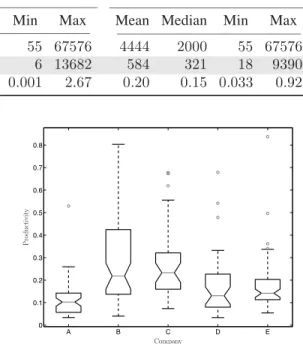
Table 2 reports basic summary statistics for both data sets. Here, effort is recorded in person hours, size in FiSMA FP (a variant of function points) and raw produc-tivity as a ratio of size to effort (i.e. FiSMA FP per per-son hour). Clearly, the distributions forFinnish788indicate the presence of inﬂuencing outliers for all three variables. The same is true forFinnish395, although to a lesser extent partly due to our data cleaning process.

1_{These are}₂₁_{ordinal variables that characterise the development}

envi-ronment, such as functionality requirements, usability requirements, anal-ysis skills of staff and their team skills.

4 Experimental Design

This section describes the methodology adopted for our experiments. To recall, the broad objective is to predict projecteffort (dependent variable) using independent vari-ables. We build the cost models using linear regression and then, evaluate and compare their performance using se-lected accuracy measures.

AlthoughFinnish395allowed over30variables to be in-cluded in the model as independents, we chose to usesize alone for two reasons.2 _{First, during a pilot of this study,}

we used forward stepwise regression that selected size as the most important factor and only two other development environment variables as independents; however, the latter added little to the model. Secondly, the complexity of build-ing a regression model usbuild-ing so many variables of mixed data types would have drifted the focus of the paper away from its intended objectives. Our intention was to keep the models easy to understand and comparable to each other.

One assumption behind building linear regression mod-els is that the included variables must be approximately nor-mally distributed. A Kolmogorov-Smirnov test (a one sam-ple test to check if a variable is normally distributed) on both, effort and size revealed that neither were normally distributed. Hence, the two variables were transformed into their natural logarithms, which were then normally distributed. The linear regression model took the form

ln(effort) =α+β ln(size), whereαis the constant andβis the regression coefﬁcient. When the model is transformed back into its original form, it converts toeffort=αsizeβ.

This model has the added advantage of investigating, whether economies of scale exist, i.e., lesser effort is ex-pended to build an additional size unit of software (function points in our case). This is exhibited whenβ < 1, since an increase of one unit in size would increase effort less than proportionally. Likewise, forβ >1an increase by one unit in size causes effort to increase more than proportionally, thus suggesting diseconomies of scale. Lastly, whenβ = 1, effort simply increases as by a multiple ofsize(α), suggest-ing constant returns to scale.

Another matter of importance are extreme values or out-liers in the data set that can cast strong influence on the regression parameters (αandβ). These must be identified and removed to increase the model’s goodness-of-fit (R2). To identify such outliers, we computed Cook’s distance (D) for each project in the data used to build the model. Then, those projects with D > 3/4n, wherenis the number of data points, were removed. Thereafter, the model was re-built without the outliers. All results reported in the paper are derived from the latter model.

Accuracy of the regression models was measured using

2_{Our data cleaning was conducted keeping further possible experiments}

(4)

Table 2. Summary Statistics for Finnish788 and Finnish395

Finnish788 Finnish395

Variable Mean Median Min Max Mean Median Min Max Effort (person hours) 3754 1551 55 67576 4444 2000 55 67576 Project Size (FiSMA FP) 584 293 6 13682 584 321 18 9390 Productivity = Size/Effort (FiSMA FP/hour) 0.22 0.16 0.001 2.67 0.20 0.15 0.033 0.92 • The percentage Pred(x)of predictions that lie within

±x%of the actual effort value (for (x= 25andx= 50)

• Mean Magnitude of Relative Error(MMRE): MMRE= 1 n n i=1 |ActualEffort_i−PredictedEffort_i| ActualEffort_i

• and Median Magnitude of Relative Error(MdMRE)for each experiment.

It is noteworthy that relative error is largely accepted as a biased statistic [5]. However, currently no universally ac-ceptable substitute is known to us and hence, we compute it for our study. Additionally, we wish to make our results comparable to studies in Section 2, since nearly all used the same accuracy measures. In Tables 3, 4, 5, and 6, we present our results using these accuracy measures. How-ever, this has been done visually to ease comparing perfor-mance of the different models.

For each experiment, we paired Pred(25)with Pred(50) andMMREwithMdMRE. Then, each pair was plotted as a bar scaled from0to1. The bars are interpreted as follows — for Pred(x), longer black bars represent higher accuracy and vice versa forMMREandMdMRE.

Pred(25); Pred(50) MMRE;MdMRE Low Accuracy

Avg. Accuracy High Accuracy

For readers interested in actual values, corresponding re-sults in tables have been provided in the Appendix section.

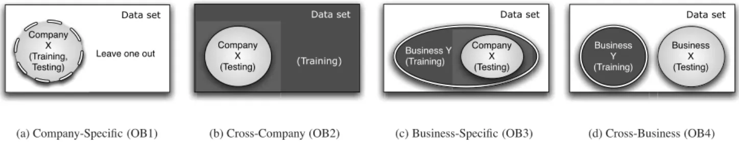
The objectives of our study require different training and testing sets to be extracted to build the cost models. These are illustrated in Fig. 1 and are described below. Note that the enumerations (i.e., (a), (b), etc.) are mapped with those of the objectives in Section 1 and the subﬁgures in Fig. 1.

(a) To achieveOB1, we ﬁrst built company-speciﬁc cost models using project data originating from a single company to predict its own projects. The models were built and evaluated using the leave-one-out method

[Fig. 1(a)]. A B C D E 0 0.1 0.2 0.3 0.4 0.5 0.6 0.7 0.8 Pro ductivit y Company

Figure 2. Company Productivity Comparison

(b) To achieveOB2, we built cost models using all data points fromFinnish395except those originating from a company, say Company X. Then the effort of each project from Company X was predicted using the model[Fig. 1(b)].

(c) To achieveOB3, we built cost models using data from exclusive business sectors, but leaving out projects from Company X. Then, individual projects from Company X were predicted for using the correspond-ing cost models of business sectors to which they be-long[Fig. 1(c)].

(d) To achieve OB4, we built cost models for each busi-ness sector exclusively and then predicted for projects from one business sector, say Business X using cost models from every other business sector other than Business X[Fig. 1(d)].

In addition to making comparable models, we wished to do the same for the results. For this, it is vital that the test set remains unchanged (except forOB4). We made this pos-sible by selecting five different companies fromFinnish395 with35or more projects that exclusively comprised five dif-ferent test sets. Thus, administering the difdif-ferent test sets to any of the above models would result in the same number of predictions, making like-for-like comparisons possible. Productivity (defined as the ratio of effort to size) compar-isons across companies is plotted in Fig. 2 where we can observe statistically significant differences.

(5)

Data set Company

X (Training,

Testing)

Leave one out

(a) Company-Speciﬁc (OB1)

Data set (Training)() Company X (Testing) (b) Cross-Company (OB2) Data set Business Y (Training) Company X (Testing) (c) Business-Speciﬁc (OB3) Data set Business X (Testing) Business Y (Training) (d) Cross-Business (OB4)

Figure 1. Training and Testing Sets for Different Cost Models Table 3. Company-Speciﬁc Cost Models

Company β Pred(25); Pred(50) MMRE;MdMRE

A 0.96 B 0.98 C 0.87 D 1.15 E 1.24 better better

5 Company-Speciﬁc Cost Models

To meet our ﬁrst objective (OB1), we built company-speciﬁc cost models to predict their own projects using the leave-out-out approach. Our results from these experiments are presented in Table 3 (and Table 7 in the Appendix).

It appears that company-specific cost models do not fare well in all cases. The Pred(x)values for companies A, B, and C indicate very weak predictive power, which is also reflected by theirMMREandMdMRE. On the other hand, cost models for companies D and E, especially for the latter, perform very well. RespectiveMMREandMdMREvalues for the two companies are also comparably low, suggesting a better model fit.

With regards to economies of scale, companies A and B showed marginal increasing returns to scale, while in the case of company C, the returns to scale were even higher. On the other hand, Companies D and E showed disec-onomies of scale. Such results partly shed light upon why in some studies, cross-company models fail to perform as well as company-speciﬁc models. Data drawn from compa-nies differing in their returns to scale may build poor models rendering them ineffective for prediction purposes. Banker et al. [2] noted that economies of scale prevails for small software projects, while diseconomies of scale exist when projects get larger in size. Investigating this case for our data set is beyond the scope of this paper since it involves building different models and deviates us from the objec-tives of our research.

6 Cross-Company Cost Models

Our second objective (OB2) was to investigate if cross-company cost models perform comparably to cross- company-speciﬁc cost models. Table 4 sums up our results, while corresponding values are shown in Table 8 in the Appendix. We see a modest improvement in the Pred(x)values for Company A, while those for companies B and C remain unchanged. The same is true for MMRE and MdMRE, which changed negligibly too for all three companies. How-ever, a marked difference in performance can be observed in the cases of companies D and E. The cross-company model appears to have considerably poor predictive power for these two companies in comparison to the company-speciﬁc model. The Pred(25)values for both fell to0, while their Pred(50)values declined appreciably as well.

Our results suggest that cross-company cost models per-form either comparably or worse than company-specific cost models, except in the case for Company A. To confirm this, we conducted a Kruskal-Wallis test3_{of significance (at}

α = 0.05) on the residuals derived using the two models on each company. The test’s results showed no significant differences in the residuals’ distribution for all, except for Company E. For the latter, the company-specific model per-formed significantly better than the cross-company model.

We also performed the statistical test on theMagnitude of Relative Error MREfor different companies using the two models. Contrary to the residuals, all comparisons were sig-niﬁcantly different with an exception of Company B, thus painting a slightly different picture. From this we learn that although, the residuals using the two models may be com-parable to each other, overall prediction accuracy is better when using company-speciﬁc cost models.

For this section, it is not meaningful to discuss economies of scale in depth because the training data came from a large number of companies (i.e. the complement of the test data fromFinnish395). But on the whole, we can observe marginally increasing or constant returns to scale.

3_{A non-parametric test comparing the medians of two distributions to}

(6)

Table 4. Cross-Company Cost Models

A 1.00 B 0.97 C 0.96 D 0.97 E 0.95 better better

Perhaps, this is an artefact of data from the different com-panies negating each other’s returns to scale.

7 Business-Speciﬁc Cost Models

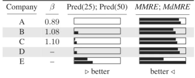
Our results from building business-speciﬁc cost models (OB3) are reported in Table 5 (see also Table 9 in the Ap-pendix). Again, like the previous two models, this one does not exhibit any consistent prediction accuracy pattern. But on the whole, it is more comparable to company-speciﬁc cost models.

The Pred(x) values for Company A are 0, while the MMREandMdMREare the poorest amongst all three mod-els. But all four accuracy measures indicate that business-speciﬁc cost models work best for companies B and C. In their case, while Pred(x)values were the highest, the MMRE and MdMRE were the lowest amongst the three models examined so far. In the case of both, Companies D and E, accuracy measures show an improvement in per-formance in comparison to cross-company cost models, but not comparable to company-speciﬁc cost models.

Again, we conducted the Kruskal-Wallis test of sig-nificance to compare residuals from business-specific cost models with company-specific cost models and cross-company cost models on the individual cross-company data. It turned out that none of the comparisons were significantly different from one another.

However, in the case of comparing MRE, all predic-tions using business-specific cost models were significantly different from company-specific cost models, with an ex-ception of Company D, while the same is true for cross-company cost models with an exception for Company E. Thus, again while residuals may not differ much from one another, there appears to be an overall difference in predic-tion accuracy.

Interestingly, we see a pattern comparable to the above two models, when examining economies of scale. Company A belonged to the Public Admin. sector which shows in-creasing returns to scale, while Banking and Insurance sec-tors (for Companies B and C respectively) exhibit slight dis-economies of scale. For Companies D and E, we report no

βvalues since the projects came from two or three business

Table 5. Business-Speciﬁc Cost Models

A 0.89 B 1.08 C 1.10 D – E – better better

sectors. In their case, projects were predicted using models trained with data from the respective business sectors.

8 Cross-Business Cost Models

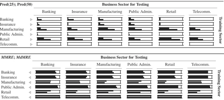
The last objective (OB4) of this paper was to investigate if cost models built using data from one business sector can be used to predict costs of projects from other sectors. Our results are shown in Table 6, where the business models in the rows are the source of training data to build the cost models, while the columns represent sectors that provide the testing data. The upper part of Table 6 shows the values for Pred(25) and Pred(50) and the lower part the values for MMREandMdMRE.

Clearly, cross-business cost models perform poorly in general. The models trained from the Banking, Insurance, Public Admin., and Telecommunication sectors give poor Pred(x) values for all business sectors, including them-selves. The same deduction can be drawn from the re-spectiveMMRE andMdMREvalues, which are consider-ably high. On the contrary, Manufacturing and Retail sector models in comparison perform more favourably, and espe-cially well for themselves giving high Pred(x)values and relatively lower residuals.

It is noteworthy that they also can predict with reason-able accuracy for the Telecommunications sector that fails to predict itself. The Telecommunication sector models consistently performed very poorly across all other sectors having Pred(x)always0%andMMREandMdMRE consis-tently over95%.

On the whole, our results do not strongly support our hypothesis that some business sectors can be gainfully used for cost modelling for other sectors. However, the Manufac-turing and Retail sectors stand out from the rest since their cost models appear to have higher predictive power than the others. We suspect that our results are an artefact of the pro-ductivity distribution across different business sectors and number of projects in each.

9 Threats to Validity

(7)

Table 6. Cross-Business Cost Models.

Pred(25); Pred(50) Business Sector for Testing

Banking Insurance Manufacturing Public Admin. Retail Telecomm.

T ra ining Se ct o r Banking Insurance Manufacturing Public Admin. Retail Telecomm.

MMRE;MdMRE Business Sector for Testing

Banking Insurance Manufacturing Public Admin. Retail Telecomm.

T ra ining Se ct o r Banking Insurance Manufacturing Public Admin. Retail Telecomm.

Threats to external validity. These threats are pertaining to the generalisations we can draw from our study. This study was conducted using a sample of only Finnish projects which certainly do not represent global development trends. All the more, these projects may not even represent the population of soft-ware projects in Finland.

Threats to internal validity. These threats pertain to our experimental procedure that might affect our results. Firstly, our data cleaning process removed of nearly half the number of projects inFinnish788. We believe that this was a necessary evil to have more faith in our results. Secondly, we only used project size as an in-dependent variable. With over30other variables to choose from, better modelling techniques can be de-veloped to accommodate more such variables to im-prove prediction accuracy.

Hence, the ﬁndings from our study are local to this very data set and needs further in-depth analysis to draw broader conclusions.

10 Conclusions and Future Work

Many studies have been conducted to determine if company-speciﬁc cost models deliver more accurate pre-dictions in comparison to cross-company cost models. Un-fortunately, mixed results have constrained the community from drawing any conclusions yet. We suspected the use of heterogenous data to build cross-company cost models, partly to be a cause for their poor performance.

Our hypothesis in this study was that building cost mod-els using more homogenous data would deliver better re-sults. For this, we built cross-company cost models us-ing data from companies belongus-ing to one business sec-tor exclusively. These models were then compared against company-speciﬁc cost models and general cross-company cost models.

We found that while none of the models in our study per-formed consistently well for all test data, company-specific cost models appeared to slightly outperform the others. Business-specific cost models seemed to perform compara-bly to company-specific cost models, but better than cross-company cost models. Unfortunately, residuals from dif-ferent models did not differ significantly, however their re-spectiveMREs did. Hence, our inference from the results is based purely on the reported accuracy measures.

Thus, while the question of ‘which model is better’ con-tinues to remain open, there is evidence that researchers should build cross-company cost models using more ho-mogenous data. Hoho-mogenous subsets can be extracted from a larger data sets using expert judgement or statistical anal-ysis. A clearer picture of this topic can perhaps be painted by replicating previous studies where cross-company data is handled more systematically, rather than as available.

Small and new software companies can substantially beneﬁt from the lessons learnt from our research. When lacking in-house project data, our results suggest that com-panies must prefer procuring data from sources that are comparable to themselves. Such data is likely to yield better estimations and in turn, better decisions.

(8)

features that could possibly contribute towards an im-proved prediction accuracy. Alternative modelling tech-niques could also shed more light on consistency of per-formance, one of them being Case-Based Reasoning [16] in which predictions are made using a local neighbourhood rather than generalised models. But more importantly, there is a need to devise a protocol for empirical studies to make them comparable to each other.

Acknowledgements.The authors thank Pekka Forselius from STTF for making the Finnish data set available to us to undertake this study. Special thanks to Christian Lindig for his bar graph macro. Thomas Zimmermann is additionally funded by the DFG-Graduiertenkolleg “Leistungsgarantien f¨ur Rechnersysteme”.

References

[1] STTF - http://www.sttf.ﬁ.

[2] R. D. Banker, H. Chang, and C. F. Kemerer. Evidence on economies of scale in software development. Information and Software Technology, 36(5):275–282, 1994.

[3] L. C. Briand, K. E. Emam, D. Surmann, I. Wieczorek, and K. Maxwell. An assessment and comparison of common software cost estimation modeling techniques. In ICSE 1999, pages 313–322, Los Angeles, May 1999. ACM. [4] L. C. Briand, T. Langley, and I. Wieczorek. A replicated

assessment of common software cost estimation techniques. InICSE 2000, pages 377–386, Limerick, June 2000. ACM. [5] T. Foss, E. Stensrud, B. Kitchenham, and I. Myrveit. A

sim-ulation study of the model evaluation criterion mmre.IEEE Trans. on Softw. Engg., 29(11):985–995, Nov. 2003. [6] R. Jeffery, M. Ruhe, and I. Wieczorek. A comparative study

of two software development cost modeling techniques us-ing multi-organizational and company-speciﬁc data. Info. and Softw. Technology, 42(14):1009–1016, Nov. 2000. [7] R. Jeffery, M. Ruhe, and I. Wieczorek. Using public domain

metrics to estimate software development effort. In MET-RICS 2001, page 16, London, Apr. 2001. IEEE.

[8] B. Kitchenham and E. Mendes. A comparison of cross-company and within-cross-company effort estimation models for web applications. InEASE 2004, pages 47–55, Edinburgh, May 2004.

[9] B. Kitchenham, E. Mendes, and G. H. Travassos. A sys-tematic review of cross- vs. within-company cost estimation studies. InEASE 2006, Keele, Apr. 2006.

[10] M. Leﬂey and M. Shepperd. Using genetic programming to improve software estimation based on general datasets. InProcs. of Genetic and Evolutionary Computation Confer-ence (GECCO), pages 2477–2487. Springer-Verlag, 2003. [11] K. Maxwell and P. Forselius. Benchmarking software

devel-opment productivity.IEEE Software, 17(1):80–88, Jan./Feb. 2000.

[12] K. Maxwell, L. V. Wassenhove, and S. Dutta. Perfor-mance evaluation of general and company speciﬁc models in software development effort estimation. Mgmt. Science, 45(6):787–803, June 1999.

[13] E. Mendes and B. Kitchenham. Further comparison of cross-company and within-company effort estimation mod-els for web applications. InMETRICS 2004, pages 348–357, Chicago, Sept. 2004. IEEE.

[14] E. Mendes, C. Lokan, R. Harrison, and C. Triggs. A repli-cated comparison of cross-company and within-company ef-fort estimation models using the isbsg database. In MET-RICS 2005, page 36, Como, Sept. 2005. IEEE.

[15] R. Premraj, M. Shepperd, B. Kitchenham, and P. Forselius. An empirical analysis of software productivity over time. In

METRICS 2005, page 37, Como, Sept. 2005. IEEE. [16] M. Shepperd and C. Schoﬁeld. Estimating software project

effort using analogies. IEEE Trans. on Softw. Engg., 23(11):736–743, 1997.

[17] I. Wieczorek and M. Ruhe. How valuable is company-speciﬁc data compared to multi-company data for software cost estimation? InMETRICS 2002, page 237, Ottawa, June 2002. IEEE.