Resource Speed Optimization for Two-Stage
Flow-Shop Scheduling
Alessandra Melani
∗, Renato Mancuso
†, Daniel Cullina
†, Marco Caccamo
†, Lothar Thiele
‡ ∗Scuola Superiore Sant’Anna, Pisa, Italy, [email protected]
†
University of Illinois at Urbana-Champaign, USA,
{
rmancus2, dcullina, mcaccamo
}
@illinois.edu
‡Swiss Federal Institute of Technology (ETH), Zurich, Switzerland, [email protected]
Abstract
Multiple resource co-scheduling algorithms and pipelined execution models are becoming increasingly popular, as they better capture the heterogeneous nature of modern architectures. The problem of scheduling tasks composed of multiple stages tied to different resources goes under the name of “flow-shop scheduling”. This problem, studied since the ’50s to optimize production plants, is known to be NP-hard in the general case. In this paper, we consider a specific instance of the flow-shop task model that captures the behavior of a two-resource (DMA-CPU) system. In this setting, we study the problem of selecting the optimal operating speed of either resource with the goal of minimizing power consumption while meeting schedulability constraints. We derive an algorithm that finds an exact solution to the problem in polynomial time, hence it is suitable for online operation even in the presence of variable real-time workload.
I. INTRODUCTION
The current trend in embedded systems industry is to exploit the high degree of parallelism offered by modern architectures. In fact, they are rich in computational resources and offer a plethora of specialized components capable of efficiently performing specific sub-tasks. For instance, in scratchpad-based architectures, data engines (DMAs) are first used to load the task to be executed, or the data to be processed, onto the scratchpad. Next, the loaded task is executed on the CPU. Similarly, if we consider hybrid CPU-GPU architectures, the CPU is responsible for device initialization and data preparation, while image processing kernels are dispatched to the GPU to boost performance. In the real-time literature, execution models [1, 2] have been proposed whose tasks are composed by two phases: a memory phase and an execution phase. During the former one, task data are loaded from main memory to cache or scratchpad memory; during the latter phase, the task is executed using the preloaded data. A precedence constraint between memory and execution phase exists because the execution of a task cannot begin before the required data have been loaded. Moreover, while the execution phase is performed on the CPU, data load can be carried out using a DMA. Thus, two phases of different tasks can be performed in parallel.
In general, the class of scheduling problems for multiple-stage jobs that execute on an ordered sequence of resources takes the name of “flow-shop scheduling”. This class of problems has been largely studied since the early ’50s because is also relevant to schedule resources and assembly phases in production plants. The problem of selecting the optimal schedule for flow-shop jobs with more than two stages, however, has been proven to be NP-hard in [3]. In this work, we focus on flow-shop tasks characterized by two stages and consider a task model where: a) each task stage requires to be executed on a specific type of resource, and b) one resource of each type exists in the system. Given this setup, we study the problem of determining the minimum speed at which one of the two resources (e.g., CPU) can be operated such that schedulability constraints are met. Specifically, we propose an on-line algorithm that, given a batch of jobs with the same deadline as input, determines the minimum (optimal) speed at which to operate the variable-speed resource subject to deadline constraints. The proposed algorithm runs in polynomial time and is thus suitable for online operation in open systems, where real-time workload changes at run-time and the system needs to adapt its scheduling policy. In order to solve the described problem and without loss of generality, we instantiate our model on a DMA-CPU scenario and derive our results assuming fixed DMA speed and variable CPU speed (the same approach can be entirely reused for an equivalent system where the speed of the first resource is varied instead). In the following, speed is quantified in terms of variable clock period of the computing resource. As clarified in Section V, this allows us to reason on piecewise linear functions, hence it is easier for the reader to follow the proposed results.
In a nutshell, this work introduces a novel and efficient (polynomial-time) algorithm that derives the optimal CPU (or memory) speed when single-rate periodic tasks that run across two stages of single-unit resources are considered.The selected optimal speed allows minimizing power consumption while ensuring that schedulability constraints are met.
Organization of the paper. The remainder of this paper is organized as follows. In Section II, we review related work. In Section III, we present the adopted system model and assumptions. Section IV establishes the necessary background. Next, we describe the proposed algorithm in Section V, while in Section VI we discuss its complexity. In Section VII we evaluate our algorithm by simulation studies. Finally, Section VIII concludes the paper and outlines future work.
II. RELATEDWORK
The flow-shop problem has been extensively studied by the combinatorial optimization community, especially in the context of production scheduling. In 1954, Johnson proposed an optimal solution to the flow-shop problem in the case of a two-stage production facility and a collection of independent jobs to be processed in sequence on the two resources [4]. More recently, the flow-shop problem has been shown to be strongly NP-hard if jobs consist of more than two stages [3], or if two or more resources are available for each stage [5]. To overcome such limitations, several heuristic solutions [6] and polynomial-time approximation schemes (PTAS) [7] have been proposed.
Lately, along with the advent of modern embedded systems, the real-time scheduling community renewed the interest towards multi-stage execution models. In the embedded and high-performance domain, co-scheduling algorithms are increasingly used to bound the memory interference due to concurrent accesses to shared memory by different cores. An attempt in this direction has been pursued by Pellizzoni et al. [1], who introduced the PRedictable Execution Model (PREM). This scheduling framework models a task as comprised of two distinct phases: a memory phase, where the task context is loaded into local memory, and an execution phase where the task executes with no memory contention. Schedulability analyses for PREM tasks have been proposed in [2, 8, 9, 10].
A number of works that focus on schedulability analysis of real-time tasks on scratchpad-based systems employ a two-stage, two-resource task model [11, 12, 13]. These works are concerned with the arrangement of scratchpad memory in space and load/unload operations in time. While we inherently share similarities in the task model adopted, to the best of our knowledge none of the existing works considers the problem of deriving the optimal speed of the two resources while satisfying real-time constraints. By restricting our setting to the case where an optimal schedule can be computed, we take a first step in this direction by deriving the minimum operating speed for the computing (or memory) resource that satisfies schedulability constraints.
III. SYSTEMMODEL
While our results can be applied to generic two-resource flow-shop tasks, we instantiate our problem on traditional computing platforms, considering DMA-CPU tasks (e.g., PREM tasks). Thus, we express tasks as composed of a memory phase (M -phase), followed by a computation phase (C-phase). More formally, we consider a setT ofnperiodic real-time tasksτ1, . . . , τn.
We assume that the two resources can operate with any value of clock period1 in the rangeT
ck ∈[1,+∞). Each task τi is
defined by a (worst-case) memory-access timeMiand a (worst-case) computation timeCi, relative to the initial configuration
where the clock period Tck is equal to1, i.e., is the minimum possible. Hence, if the objective is to optimize the speed of
the first (resp., second) resource, the memory-access time Mi (resp., computation timeCi) of each task is linearly scaled2 as Mt
i =Mi·t (resp., Cit=Ci·t) for any value of Tck =t ≥1, while the speed of the other resource is kept constant. The
underlying assumption is that, in the considered platform, the speed of each resource can be varied continuously. Albeit this is not true in general, it is worth noticing that increasing attention is given to advanced power scaling features in all modern architectures, from embedded platforms to data-centers. Since operating frequency is known to have a directly proportional impact on power consumption [14], modern platforms are endowed with Dynamic Voltage and Frequency Scaling (DVFS) units that allow live adjustments of the operating frequencies at a high granularity. For example, the Nvidia Tegra K1 SoC3 is a hybrid CPU-GPU architecture designed for embedded applications that allows for nine levels of frequency scaling on its low-power CPU cores, twenty levels for its high-power CPUs and fifteen levels for its GPU. Similarly, the Intel i7 4770K4, designed for workstation machines, provides sixteen frequency scaling levels.
While frequency scaling is an effective way to scale performance and power consumption on CPUs, DMA engines are regulated using bandwidth control (BWC) features instead. BWC features allow specifying the number of intermediate idle states between every block of transferred bytes in a DMA operation. Since both the transfer block size and the number of idle states are a configurable parameter, BWC features provide a high granularity of performance scaling. For instance, the Freescale MPC5777M SoC5 can be configured to perform DMA operations with up to eight idle states between two memory
transactions, and with block sizes ranging from 1 byte to 16 bytes. Similarly, the Freescale P40806 features eleven levels of
DMA throttling with four configurable transfer block sizes.
We assume that all tasks share the same relative deadlineD, which is constrained to be smaller than or equal to their period
T. Therefore, starting from an arbitrary time r when all tasks release their first job, subsequent job releases of all tasks will 1Although reasoning in terms of clock periodT
ckdescribes well the performance of CPUs, it is more appropriate to reason in terms of bandwidth when
describing the performance of memory subsystems. However, since a dualism exists between the two concepts, we will adopt the notationTckwhen referring
to either resource type.
2Computation is performed over data that has been preloaded into local memory, while memory operations do not involve computation. Thus computation
time scales linearly with clock speed as long as CPU speed and local memory are tied to the same clock. Similarly, performance of memory-only operations scales linearly with the configured transfer bandwidth.
3See http://www.nvidia.com/object/tegra-k1-processor.html 4See http://ark.intel.com/products/75123/Intel-Core-i7-4770K
5See http://cache.freescale.com/files/32bit/doc/fact sheet/MPC5777MFS.pdf 6See http://cache.freescale.com/files/32bit/doc/prod brief/P4080PB.pdf
happen at timesr+kT, being kany positive integer. Each job released byτi first executes itsM-phase on a data processor,
and then executes itsC-phase on a CPU. Thus,M-phases (C-phases) of a given taskτican progress in parallel withC-phases
(M-phases) of a different taskτj.
Since in our model tasks are synchronously released and have the same deadline D, preemption does not provide any schedulability advantage. Thereby, our results do not use preemption. Also, modeling resources as non-preemptive allows capturing the realistic behavior of some resources. For instance, DMA operations can be aborted/canceled, but it is often not safe to assume that a certain amount of data has been successfully transferred.
For a given schedule of jobs in a period, themakespanis defined as the time between the release of the jobs and the completion of theC-phase of the last job in the schedule. In this setting, the schedulability problem (i.e., verify whether deadlines are met) is equivalent to the problem of makespan minimization, for which an optimal solution that runs in polynomial time exists [4]. More specifically, since one job of each task is released at multiples ofT, it is enough to compute the (optimal) makespan of such collection of jobs and check it against the global relative deadlineD=T to verify the schedulability of a given task-set. Since the execution pattern repeats identically in each period, we can restrict our analysis to consider only the first instance of each task, denoting such a collection of jobs as J1, . . . , Jn. Without loss of generality, we assume all such jobs to be released
at time0 and to have deadline at timeD.
We remark that, when more general task models are considered, the problem loses some of the desirable properties it has in the case of two resources and two-stage tasks. We previously mentioned that the makespan minimization problem becomes NP-hard when each task consists of more than two phases [3] or when two or more resources are available for each stage [5]. Moreover, if tasks do not share the same period/deadline, the schedulability problem is no longer equivalent to that of makespan minimization, and since no optimal scheduling algorithm is known for the general schedulability of multi-stage tasks, it is nontrivial to extend our results to more general settings while preserving optimality.
Nonetheless, despite the negative results on the tractability of the problem in the generic case, significant performance gains can be achieved by devising novel co-scheduling policies able to exploit the potential parallelism and energy saving offered by modern embedded architectures. This work is a first step to address the broader problem of speed selection for the class of multi-stage execution models. We envision that future research can extend this work to the scheduling of three-stage jobs (under certain assumptions [4]), and to optimally adjust speed of multiple resources. Finally, while extending the task model to arbitrary periods is not needed for practical purposes, we plan to extend it to support a limited set of task rates. For instance, our approach could be reused with different job rates on a multicore platform if each rate group is scheduled in isolation on private hardware resources (core with dedicated DMA channel).
IV. BACKGROUND
In this section, we provide the necessary background for the reader to understand the analogies of our scheduling problem with the well-known “flow-shop” problem.
A. Johnson’s algorithm
Johnson’s algorithm [4] provides an optimal solution to schedule a collection of same-deadline, time-synchronized two-resource tasks. The following theorem defines the relative ordering between pairs of jobs in an optimal schedule.
Theorem 4.1: (from [4]) Given a collectionJ1, . . . , Jn of two-stage flow-shop jobs,Ji precedes Jj in an optimal schedule
if
min(Mi, Cj)<min(Mj, Ci). (1)
The steps of Johnson’s algorithm for constructing an optimal schedule are the following:
1) Partition the jobs into two sets S1 andS2.S1 contains the jobs having Mi< Ci,S2 contains the jobs with Mi > Ci.
The jobs withMi=Ci may be put in either set;
2) Jobs inS1 are sorted in increasing order, while jobs inS2 are sorted in decreasing order; 3) The final ordering is obtained by concatenating the two sequences as S= [S1;S2].
The cost of sorting the two sets dominates over other operations, hence the time complexity of Johnson’s algorithm is
O(n log(n)). In the rest of the paper, we will denote asσt={σt
1, . . . , σtn}the permutation of jobs that determines the optimal
schedule when Tck=t.
B. Computing the optimal makespan
Given an optimal job ordering σt={σt
1, . . . , σtn}, the corresponding value of makespanµt is given by:
µt=maxn i=1 i X j=1 Mj+t· n X j=i Cj . (2)
M2 M3 M1 C1 C2 C3 a) b) c) M2 M3 M1 C1 C2 C3 M2 M1 M3 C2 C1 C3 d) M2 M1 M3 C2 C1 C3
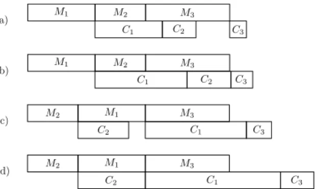
Fig. 1. Example of a task-set composed of three tasks with parametersτ1= (4,4),τ2= (3,2),τ3= (5,1). The four insets illustrate the optimal schedule
when a)Tck= 1; b)Tck= 1.33; c)Tck= 1.5; d)Tck= 2.
This expression gives us many insights. Specifically, it indicates that an optimal schedule has the following characteristics: (i) there are no internal gaps in the use of either resource; (ii) there exists a critical path that determines the minimum makespan; (iii) such a critical path can be determined by identifying a crossover job J∗
i such that jobs preceding it in the
optimal schedule contribute to µt with their memory-access time, while subsequent jobs contribute with their computation
time; (iv) J∗
i contributes toµ
twith both M
i andCi.
Note also that Equation (2) can be implemented efficiently, that is, to run in linear time in the size of the task-set. V. OPTIMAL RESOURCE SPEED SELECTION
In this section, we present our algorithm to derive the minimum resource speed that guarantees the schedulability of a given task-set. In the rest of the paper, we will denote as FC(t)(resp.,FM(t)) the function that associates the value of the optimal
makespan to any value of clock periodTck=twhen variations in the speed of the second (resp., first) resource are considered.
For ease of understanding, we will instantiate the problem in the case of a fixed DMA speed and a variable CPU speed, and then show how to reuse the same approach when considering variations in the speed of the first resource.
For any fixed value ofTck, Johnson’s algorithm (see Section IV-A) can be used to find the job ordering that corresponds to
the minimum makespan. However, as the clock period is scaled, the value of the optimal makespan increases, due to the scaling factor applied to computation times. Additionally, depending on the scheduling decisions imposed by Equation (1), jobs can be possibly rearranged in a different order. As an example, consider a task-set composed of three tasks τ1= (M1, C1) = (4,4),
τ2 = (3,2) andτ3= (5,1), with T =D = 20. Initially, whenTck = 1, Johnson’s algorithm orders the jobs as depicted in
Figure 1(a), with J3 being the crossover job. The optimal makespan, equal to 13, can be found by Equation (2), where the maximum is achieved fori= 3. As the clock period is scaled, the optimal makespan linearly increases, due to the inflation of the
C-phase ofJ3. However, when the value ofC1+C2reaches that ofM2+M3, i.e., whenTck= (M2+M3)/(C1+C2) = 1.33,
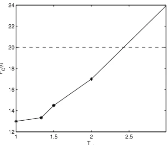
J1 becomes the crossover job, as shown in Figure 1(b), and the makespan increases at a higher rate. Then, as soon as the computation time of τ2 reaches the value of its memory-access time (i.e., whenTck =M2/C2 = 1.5), Johnson’s algorithm imposes a job reordering (see Figure 1(c)) that reduces the makespan growth rate. Finally, the rate of the optimal makespan will increase again as soon as C2 reaches the value ofM1, i.e., when Tck=M1/C2= 2, because from this point there is no gap in the processor usage, and all three jobs will contribute to the makespan with their computation times (see Figure 1(d)). Figure 2 illustrates the function FC(t) for the example above. We can immediately observe that such a function: (a) is
monotonically increasing; (b) is piecewise linear; and (c) the points where its slope changes (i.e., Tck ={1.33,1.5,2}) are
exactly those described in Figure 1. The intersection point between this function and the horizontal line corresponding to the relative deadline gives the minimum processor speed (i.e., the maximum clock period) that optimizes the power consumption while ensuring the schedulability of the considered task-set.
In the rest of the paper, we will denote aschanging pointsthose values ofTckwhere the slope ofFC(t)changes. As evident
from the example of Figure 1, changing points may be of two types, according to the following definitions.
Definition 5.1 (Schedule changing points): Aschedule changing pointis a value of clock periodt˜of the form Mi/Ci, for
somei∈[1, . . . , n], such thatlimt→t˜−FC0(t)>limt→t˜+FC0(t)(i.e., the slope ofFC(t)decreasesin correspondence oft= ˜t). Definition 5.2 (Crossover changing points): Acrossover changing pointis a value of clock periodˆt of the form7
Mσtˆ i+1+. . .+Mσ ˆ t i+k+1 Cσˆt i +. . .+Cσ ˆ t i+k ,
for some i ∈ [1, . . . , n] and some k ∈ [0, . . . , n−i], such that limt→tˆ−FC0(t) < limt→tˆ+FC0(t) (i.e., the slope of FC(t) increases in correspondence oft= ˆt).
7We recall thatσt
1 1.5 2 2.5 12 14 16 18 20 22 24 T ck FC (t)
Fig. 2. Example of the functionFC(t)associating the clock periodTckto the value of the optimal makespan for the task-set in Figure 1. The horizontal line
corresponds to the relative deadlineD= 20. The portion of the function lying below the line identifies the values ofTckthat make the task-set schedulable.
Intuitively, schedule changing points correspond to values of clock period at which a job reordering occurs according to Johnson’s algorithm. The slope of FC(t)decreases after a schedule changing point because, if a reordering takes place in the
optimal schedule, then the minimum makespan in the new configuration must be strictly dominated by the previous one. The next lemma shows that a job may change its position in an optimal schedule only when its computation time becomes equal to its memory-access time.
Lemma 5.1: For any pair of jobsJiandJj, such thatJiprecedesJj in an optimal schedule atTck=t0 ≥1, a job swapping
may occur in the interval Tck∈(t0,+∞)only atTck=t00=Mj/Cj, provided thatt00> t0.
Proof: Without loss of generality, assume that, for Tck = t0, the C-phases of the two jobs are both shorter than the
corresponding M-phases, because otherwise Johnson’s algorithm would sort them in ascending order by the length of their
M-phase, and no reordering would be possible. Since in the initial orderingJi precedes Jj, it must also hold thatCj < Ci.
Therefore, we just need to consider the two following initial configurations: i)Cj < Ci< Mi< Mj; ii)Cj< Ci< Mj < Mi. Case i). TheC-phases of the two jobs are sorted in descending order, while theirM-phases are sorted in ascending order. It trivially follows by Johnson’s rule that no job reordering is possible for any value of t00> t0.
Case ii). By linearly increasingCi andCj, no job swapping may occur until the relative ordering between task parameters
changes. When Ci reaches the value ofMj (say, atTck=t1=Mj/Ci), a new configuration is produced, i.e.,Ct
1
j < Mj < Ct1
i < Mi. By Equation (1) we get: min(Mi, Ct
1
j ) = Ct
1
j < min(Mj, Ct
1
i ) = Mj, i.e., no reordering takes place. Next, a
different configuration is produced at Tck =t2 > t1 when either: a) the C-phase of Jj becomes larger than Mj, leading to Mj< Ct
2
j < Ct
2
i < Mi; b) the C-phase ofJi becomes larger thanMi, leading toCt
2
j < Mj< Mi< Ct
2
i .
In case ii.a), it follows by Equation (1) that a job swapping occurs at Tck =t2 =Mj/Cj. From this point on, Mj will
always lead the minimum in Equation (1), hence no further update is possible.
In case ii.b), it follows by Equation (1) that no reordering takes place for Tck=Mi/Ci. However, when atTck=t3> t2
the C-phase ofJj reaches the value of Mj, Johnson’s rule imposes a job swapping. Arguing similarly as in case ii.a), we
conclude that no further reordering is possible for Tck> t3.
Having proved that a job reordering may occur only at Tck=Mj/Cj, the lemma follows.
On the other hand, crossover changing points correspond to clock periods at which the crossover job changes. In other words, when some of the gaps in the processor usage are filled, a larger number of jobs could start contributing to the makespan with their computation times. To better clarify the difference between the two sets of changing points, consider again the example in Figures 1. Here, 1.5 is a schedule changing point, while 1.33 and 2 are crossover changing points. Note also that when
Tck ∈ [1,1.33), the slope of FC(t) is given by C3, as J3 is the crossover job, while when Tck ∈ [1.33,1.5), FC(t) starts
increasing with a larger slope (P3
i=1Ci), since now J1 has become the crossover job.
The next lemmas justify the relation between each type of changing point and its effect on the slope of FC(t). Lemma 5.2: In correspondence of a schedule changing point, the slope ofFC(t)can onlydecrease.
Proof: Each schedule changing point determines a job reordering. By contradiction, assume that after any schedule changing point the makespan starts increasing at a higher rate (i.e., more jobs start contributing to FC(t)) until the subsequent
changing point is reached. This would contradict the optimality of FC(t), because, by keeping the previous job ordering, the
makespan would increase at a smaller rate. It then follows that a schedule changing point can only determine a slope decrease of FC(t).
Lemma 5.3: In correspondence of a crossover changing point, the slope ofFC(t)can onlyincrease.
Proof: The lemma trivially follows by observing that a gap in the processor usage is closed in correspondence of each crossover changing point, but the job ordering remains the same. This means that when a crossover changing point is reached,
a larger number of jobs start contributing to the makespan increase rate, hence the slope of FC(t)can only increase.
The two lemmas above can be applied to the example of Figure 2 to visually identify schedule and crossover changing points.
A. Finding changing points
We now describe how, for a given collection of jobs, the changing points ofFC(t)can be computed.
a) Schedule changing points: To compute the list of schedule changing pointsPs, we first define a listCPsofcandidate schedule changing points:
CPs={Mi/Ci|Mi> Ci, i= 1, . . . , n}. (3)
The list of candidates CPs may be larger thanPsbecause not necessarily a job reordering takes place when the computation
time of a jobJi reaches the value ofMi. In fact, it may happen that the precedence relations imposed by Equation (1) remain
unchanged, meaning thatJi is already in its “right position” with the current ordering. In this case,Mi/Ci does not represent
a schedule changing point.
The listPscan be identified starting fromCPsas described in Algorithm 1. The algorithm returns two pieces of information.
First, it provides the list of schedule changing pointsPsordered according to their occurrence as the clock period is scaled in (0+,+∞). Second, the algorithm generates a list of schedulesS. Each element ofScorresponds to the schedule that minimizes the makespan for all values t of clock period in the interval[Ps,i,Ps,i+1). In other words, it always holds that Si =σt for
Ps,i≤t <Ps,i+1.
Algorithm 1 Computation of the listsPs andS 1: procedureSCHEDULEPOINTS(T)
2: B←DSORT(T, key=Ci)
3: E←ASORT(T, key=Mi)
4: SW ←ASORT(T, key=Mi/Ci)
5: L←ARRAY(size=n,value=null)
6: S←B;Ps← {0};f← −1 7: forj= 1tondo 8: r←SWj.M/SWj.C 9: k←INDEXOF(SWj, E) 10: Lk←SWj 11: B←REMOVE(SWj, B)
12: L0←FILTER(L,value=null)
13: σcurr←CONCAT(L0, B)
14: ifσcurr6=LAST(S)then
15: Ps←APPEND(r,Ps) 16: S←APPEND(σcurr, S) 17: iff=−1andr≥1then 18: f←r 19: end if 20: end if 21: end for 22: {Ps, S} ←REINIT(Ps, S, f) 23: return{Ps, S} 24: end procedure
Algorithm 1 first constructs the beginning and ending optimal schedules for values ofTck ranging in(0+,+∞). According
to Equation (1), when the computation time Ci of each job is shorter than its corresponding memory-access time Mi, the
optimal schedule is obtained by sorting the jobs byCi in descending order. Thus, this schedule is the initial one forTck≈0+,
and is calculated as B at line 2, and also stored as first element ofS at line 6. Similarly, for Tck≈+∞, the jobs are sorted
in ascending order according toMi. This sequence is calculated and stored into Eat line 3. The key idea to find the schedule
changing points is to observe that each candidate is associated to a single job, and, by Johnson’s rule, if a schedule changing point occurs atTck=t, only the associated job will swap position fromσt
−
toσt. Intuitively, this is because when a schedule
changing point for job Ji is reached, the result of the comparison in Equation (1) may change, thereby determining a new
position of Ji within the schedule, as depicted in Figures 1(b) and 1(c). Hence, by sorting the candidate changing points in
ascending order, we can build a list of possibly swapping jobsSW (line 4).
It also follows from Johnson’s rule that any job that has passed its own schedule changing point (i.e., whoseC-phase has become longer than its M-phase) will appear in the schedule before any job that has not passed it. In fact, consider a job
Ji that has passed its schedule changing point. A second job Jj can only appear before Ji in the schedule σt if Mj < Mi.
However, if Cj< Mj, thenτj will be computation-dominated and always scheduled afterJi.
Therefore, in the for loop at lines 7-21, we distinguish between jobs that have passed their schedule changing point and jobs that have not. It is enough to order the former class in ascending order by Mi and the latter class in descending order
by Ci. The concatenation of the two sets will represent the optimal schedule at Tck =t. The array L, initialized at line 5,
will progressively store the jobs that have passed their schedule changing point. To prevent reordering at every step, jobs are positioned in Lat the same index they have in the final sequenceE and they are removed from B (lines 9-11). The filtering onLis needed to remove placeholdernullobjects and construct a valid candidate schedule (line 12). Maintaining empty slots (null) for all the jobs that have not reached their respective schedule changing point allows preserving the relative ordering and thus avoiding additional sorting operations.
If the schedule σcurr obtained at line 13 is different from the previously generated one, i.e., LAST(S), it follows that r
indeed represents a schedule changing point. This check is performed at line 14. If the check is passed, the listsPsandS are
updated accordingly (lines 15 and 16). Finally, since we are only interested in the changing points within[1,+∞), all points below 1should be discarded. At line 22, the function REINIT filters the points, based on the first element to consider (i.e.,f
at line 18), setting 1 as first element ofPsand updating S accordingly.
Finally, the algorithm returns as output the two lists at line 23.
b) Crossover changing points: Since a job reordering occurs only in correspondence of schedule changing points, the optimal schedule never changes between pairs of adjacent schedule changing points. Then, to characterizeFC(t), it is necessary
to find the crossover changing points falling between each pair of adjacent elements in Ps, i.e., in any interval of the form [Ps,i,Ps,i+1)8. The challenging task is then to predict in which order the gaps in the processor usage are filled as the clock period is scaled. Indeed, the number of crossover changing points strictly depends on the order in which the gaps are filled. If they are filled in order, starting from the last job in the schedule, distinct crossover changing points are generated, because the slope of FC(t) increases when each of the gaps is filled. If they are filledout of order, a crossover changing point may
be generated only when the first of the considered jobs becomes the crossover job.
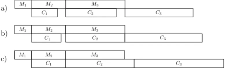
We provide some intuition of the problem by means of a simple example. Consider a task-set composed of three tasks, with the following parameters: τ1 = (M1, C1) = (2,3), τ2 = (4,6) and τ3 = (7,8). The job ordering that minimizes the makespan with Tck = 1is illustrated in Figure 3(a). In the initial configuration, J3 is the crossover job, hence it is the only one that contributes to the makespan rate with its computation time. However, when Tck reaches the value M3/C2 = 1.17 (Figure 4(b)), J2 becomes the crossover job, hence 1.17 is a crossover changing point ofFC(t). Finally, whenTck becomes
equal to M2/C1= 1.33(Figure 3(c)), the slope of FC(t)is further increased, because alsoJ1 starts affecting the makespan increase rate, becoming the crossover job. Therefore, also 1.33 can be classified as a crossover changing point of FC(t). In
this scenario, two crossover changing points are found because the gap in the processor usage relative to C2 is filled before the one relative to C1.
However, if we change the computation time ofτ2to be4instead of6, as in Figure 4(a), we observe that whenTck reaches M2/C1 = 1.33 (Figure 4(b)), the gap corresponding to C1 is filled, but no crossover changing point is generated, because the makespan increase rate is not affected by the aggregation between the two jobs. Indeed, before and after 1.33 only J3 contributes to increase the makespan rate with its computation time. Finally, when Tck = (M2+M3)/(C1+C2) = 1.57, a single crossover changing point is generated, asJ1 becomes the crossover job and all three jobs start contributing to increase the slope ofFC(t)with their computation times, as in Figure 4(c).
a) M1 C1M2 C2M3 C3 b) c) M1 M2 M3 C1 C2 C3 M1 M2 M3 C1 C2 C3
Fig. 3. Example of a task-set composed of three tasks with parametersτ1= (2,3),τ2= (4,6),τ3= (7,8). The three insets illustrate the optimal schedule
when a)Tck= 1; b)Tck= 1.17; c)Tck= 1.33. a) M1 M2 M3 C1 C2 C3 b) c) M1 M2 M3 C1 C2 C3 M1 M2 M3 C1 C2 C3
Fig. 4. Example of a task-set composed of three tasks with parametersτ1= (2,3),τ2= (4,4),τ3= (7,8). The three insets illustrate the optimal schedule
when a)Tck= 1; b)Tck= 1.33; c)Tck= 1.57.
8For the last element ofP
This example shows that the number of crossover changing points strictly depends on the order in which the gaps in the processor usage are filled. In the example of Figure 3, the two gaps are filled in sequence (in order), becauseM3/C2> M2/C1. In this case, two distinct changing points are generated, because the slope of FC(t)increases when each of the two gaps is
filled. In the second case, instead, M3/C2 < M2/C1, implying that the gaps are filledout of order: first, the gap relative to
C1 is closed, and then the makespan starts increasing at a higher rate when C1+C2 becomes equal to M2+M3, i.e., in correspondence of the (unique) changing point atTck= 1.57.
Relying on these observations, Algorithm 2 derives the sublist of crossover changing points falling inside any interval
[Ps,i,Ps,i+1). The algorithm takes as input the initial task-set T, the listPs, the index therein representing the left endpoint
Algorithm 2 Crossover changing points in[Ps,i,Ps,i+1)
1: procedureCROSSOVERPOINTS(T,Ps,i,S)
2: t← Ps,i;ρ← ∅;σt←Si
3: Z←ADJACENTJOBS(T, σt)
;D←0;N←0
4: forj=SIZE(Z) to 1do
5: ifj6=SIZE(Z)andt·Zj.ck > ϕ.ckthen
6: ifi==SIZE(Ps)orϕ.ck <Ps,i+1then
7: ρ←APPEND(ϕ, ρ) 8: end if 9: D←0;N←0 10: end if 11: D←D+C(Zj.jobs) 12: N ←N+M(Zj.jobs) 13: ϕ.ck=t·(N/D);ϕ.x←Zj.jobs1 14: end for
15: ifi==SIZE(Ps)orϕ.ck <Ps,i+1 then
16: ρ←APPEND(ϕ, ρ)
17: end if 18: returnρ
19: end procedure
of the interval, and the list of optimal schedulesS. It produces in output a structureρof crossover changing points, where the fieldρ.ckstores their values, while the fieldρ.x contains the index of the crossover job in the optimal schedule. As explained in Section VI, this is needed to efficiently compute the value of FC(t)once the list of changing points is known.
At line 3, the gaps in the processor usage are computed by the function ADJACENTJOBS, which initializes the structureZ
as follows. The field Z.jobs stores the groups of jobs whose C-phases are executed consecutively in the optimal schedule, with the exception of the last group, which may not give rise to a gap in the processor usage (e.g., C3 in Figure 1(a)). The field Z.ck stores instead the values of clock period at which the gaps are closed. Each of such values Zj.ck can be
computed as M(Zj.jobs)
C(Zj.jobs), where the operatorsM(J)andC(J)take as input a groupJ of sadjacent jobs in σ
t of the form J ={σt
k, . . . , σ t
k+s−1}and are defined as follows:
C(J) = k+s−1 X h=k Cσt h; (4) M(J) = k+s−1 X h=k Mσt h+1. (5)
Note that the index shift in Equation (5) (i.e., σt
h+1 instead ofσht) complies with the notion of crossover changing point
given in Definition 5.2.
As an example, the function ADJACENTJOBS applied to the input task-set in Figure 1(a) returns: Z.jobs ={{1,2}} and
Z.ck ={(M2+M3)/(C1+C2)} ={1.33}. Applied to the task-set in Figure 3(a), the result is: Z.jobs ={{1},{2}} and
Z.ck={M2/C1, M3/C2}={1.33,1.17}.
The variableN (resp.,D) is used to compute the numerator (resp., denominator) of the partially computed changing point, stored in ϕ.ck, while ϕ.xkeeps track of the current index of the crossover job. In the for loop at lines 4-14, the structureZ
of adjacent jobs is walked backward. If the currently examined group Zj is not the last one, and its value of clock period is
greater than ϕ.ck, it means that the gap corresponding to Zj will be filledlater than the one relative toϕ(i.e.,in order), and
the two groups of jobs will give rise to two distinct crossover changing points. Hence, ϕis appended toρ, provided that the check at line 6 is passed. This check ensures that the newly computed changing point does not exceed the right endpoint of the intervalPs,i+1. The check is trivially passed if the last schedule changing point is considered, because the right endpoint
If the check at line 5 fails, it means that the processor gap corresponding to Zj will be filledbeforethe one relative toϕ,
hence the two groups of jobs will generate a single changing point. At lines 11-13, the intermediate values of D andN are updated using the operatorsC(J)andM(J), and the new value ofϕ.ckis computed. The ratioN/D is scaled bytto account for the inflation of computation times occurred in the interval [1,Ps,i), as the crossover changing points in each interval are
initially computed with respect toPs,i. Also,ϕ.xis updated with the new index of the crossover job, given by the first element
of Zj.jobs. After thefor loop, the last crossover changing point is appended toρ(subject to the same check performed at line
6), which is finally returned as output.
B. Complete algorithm
We now describe the complete algorithm to derive the list P of changing points ofFC(t). First, the listPs is computed by
Algorithm 1, then Algorithm 2 is iteratively invoked to derive the crossover changing points in each interval[Ps,i,Ps,i+1). Algorithm 3 Computation of the listP
1: procedureCHANGINGPOINTS(T) 2: {Ps, S} ←SCHEDULEPOINTS(T);P ← Ps,1 3: P ←APPEND(CROSSOVERPOINTS(T,Ps,1, S),P) 4: fori= 2 to SIZE(Ps)do 5: P ←APPEND(Ps,i,P) 6: T0←SCALEJOBS(T,Ps,i) 7: P ←APPEND(CROSSOVERPOINTS(T0,Ps, i, S),P) 8: end for 9: returnP 10: end procedure
The pseudo-code is shown in Algorithm 3. At line 2, Algorithm 1 is invoked to compute the list of schedule changing points Ps, andP is initialized with its first value (we recall that by constructionPs,1= 1). Then, at line 3, Algorithm 2 is initially invoked with i= 1, and then thefor loop at lines 4-8 iterates on the subsequent schedule changing points. At each iteration, the i-th point in Ps is appended to P, and a new task-set T0 is obtained by scaling the original computation time of each
task by the value of Ps,i, to account for the inflation occurred in the previous interval (line 6). Then, the crossover changing
points in [Ps,i,Ps,i+1)are computed and appended toP, which is finally returned as output.
Since FC(t)is a piecewise linear function, it can be completely specified by computing its value in correspondence of all
changing points, and determining the slope of the last piece. As the optimal job ordering is known for all values of Tck (it
only changes in correspondence of schedule changing points), Equation (2) can be applied to find the value ofFC(t)for each
changing point. The slope of the last piece is simply given byPn
i=1Ci, because, in the final schedule, the computation times
of all jobs contribute to the makespan (e.g., see Figure 1(d)).
C. Scaling the speed of the first resource
We now consider variations in the speed of the first resource, that is, we seek to find the functionFM(t), assuming a fixed
CPU speed while varying the DMA speed. This function can be simply derived once the list P ={p1, . . . , p`} of changing
points of FC(t)is known9. Thus, we adapt the original system as follows.
First, we establish the initial parameters corresponding to the configuration Tck = 1. Since we are interested in scaling
memory-access times, we set the computation time C0
i of each job Ji by imposing a fixed CPU speed β ≥ 1, such that C0
i =β·Ci. Next, we select the starting point for the DMA speed as a fractionαof the original value, with0< α≤1, such
that M0
i =α·Mi. In this new setting, computation times are kept constant, while memory-access times are scaled as Mi0·t
for any value of Tck=t.
The list of changing points ofFM(t)is then given byP0 ={p01, . . . , p0`}, whose generic elementp0j is equal to: p0 j = 1 p`−j+1 ·β α.
Intuitively, this means that the changing points inP0can be simply found as the reciprocal of those inP, up to a multiplicative factor given by the choice of the initial parameters. Due to this correspondence, the points inP0are indexed in reverse order with respect toP. It is then necessary to discard all points<1fromP0to restrict the domain of the function to the interval[1,+∞). As before, Equation (2) can be used to find the value ofFM(t)in correspondence of each changing point. Symmetrically, the
slope of its last piece is given byPn
i=1Mi.
9Here, we refer to thecompletelist of changing points ofF
C(t), i.e., including all changing points in the intervalTck∈(0+,+∞). This means that,
VI. COMPLEXITY
We now derive bounds on the maximum number of changing points of FC(t)(equivalently,FM(t)). Lemma 6.1: FC(t)contains at mostn−1 schedule changing points.
Proof: The number of schedule changing points is maximized when the maximum number of swaps between jobs is necessary to reach the final schedule, where M-phases are sorted in ascending order. Such a worst-case configuration corresponds to the one where: (i) for any job Ji, Ci < Mi, i.e., in the initial optimal schedule, all jobs are
computation-dominated (hence sorted by decreasingCi), and (ii)M-phases are also sorted in descending order. In this case, it is immediate
to see thatn−1 moves are necessary to reorder the jobs as in the final schedule, proving the lemma.
Lemma 6.2: Between any two adjacent schedule changing points of FC(t), there are at most n−1 crossover changing
points.
Proof: The worst-case scenario that maximizes the number of crossover changing points in any interval[Ps,i,Ps,i+1) is given by the situation in which there are n−1 gaps in the processor usage that are closed in order. The last job is excluded (leading to a bound of n−1 instead of n) because, as previously observed, it may not give rise to a gap in the processor usage.
By combining the two lemmas above, it follows that the number of changing points is quadratic in the number of jobs. A bound on the time complexity of the complete algorithm is then given by O(n2). Indeed, the complexity of Algorithm 1, which finds the listPs, isO(n2), because thefor loop at lines 7-21 iteratesntimes, and at each iteration the cost of filtering
the arrayLat line 12, also linear in the number of tasks, dominates over the other operations. The cost of finding the crossover changing points is also quadratic, because Algorithm 3 invokesn−1times Algorithm 2, which in turn has a linear cost, since the for loop at lines 4-14 iterates ntimes and each iteration has a constant complexity. Note that the operations at lines 11 and 12 do not increase the complexity of the algorithm, because the operators C(J) andM(J) are applied to disjoint sets that have an aggregate cardinality n−1.
Note also that since Algorithm 2 keeps track of the index of the crossover job for each crossover changing point, it is then sufficient to compute the value of the optimal makespan µt only in correspondence of the schedule changing points (which
can be done in O(n2)), and then update its value for each crossover point (based on the knowledge of the crossover job), which requires O(n2)overall. In this way, the complexity remains quadratic in the task-set size.
While our algorithm derives the functionFC(t)(or, equivalently,FM(t)) analytically, a na¨ıve approach would be to perform
a binary search on the clock period domain, trying to find the optimal value of Tck that guarantees the schedulability. Such
an approach would require to select a quantization step and to run Johnson’s algorithm at each point. Beside having a high computational cost, this solution could imply some technical difficulties, mainly due to the non-convexity of the functions. Also, this method would only be able to identify the optimal solution up to the size of the quantization step.
A final remark concerns the applicability of our method also when considering systems having a small numberk << nof speeds. In this case, the computation of the schedule changing points would require O(n log(n))for the sorting at line 4 of Algorithm 1, which dominates the cost of the filtering at line 12, given byO(nk), as it should be performed onlyktimes. The computation of crossover changing points should be performed only once, i.e., for the interval[Ps,i,Ps,i+1)that delimits the optimum. Hence, the complexity would be comparable to running Johnson’s algorithm k times, but without any dependence on the number of available speeds.
VII. EVALUATION
In this section, we evaluate the performance of our approach by simulation studies. First, we describe a representative example that shows the power and energy savings that can be achieved when our algorithm is used to determine the optimal operating speed of the CPU. Specifically, we perform a comparison with simple heuristic-based scheduling strategies. Then, we quantify the schedulability advantage of the proposed optimal scheduling strategy by means of extensive simulations.
The first experiment has been performed by assuming specific energy and power models. Such models have been derived using an embedded platform and a realistic image processing benchmark. Since we are interested in optimizing power and energy consumption for the second resource (CPU), we first derive extract the power/energy profile of the considered benchmark on the hardware platform. Next, we assume that a generic synthetic taskset exhibits the same energy profile. This approach allows us to both reason about a realistic power-frequency relationship while presenting results that have nicer mathematical properties.
More in detail, we have considered an image processing benchmark, called Disparity, from the San Diego Vision Benchmark Suite [15]. The Disparity benchmark represents a data-intensive application that processes two images taken from different locations and extracts depth information to construct the position of objects depicted in the input images. For the measurements, we have used a Odroid-U3 embedded platform. The system features a Samsung Exynos 4412 processor with four ARM Cortex-A9 cores. Although the nominal maximum speed is 1.7 GHz, the CPU can be overclocked up to a frequency of 2 GHz. Moreover, the power management circuitry allows a minimum operating frequency of 200 MHz, with a scaling granularity of 100 MHz. Thereby, 20 different levels of frequency scaling can be selected. In our experiments, for each available scaling frequency, we
execute the aforementioned benchmark and record: (a) the current I flowing to the system; and (b) the execution time R of the benchmark under analysis. Finally, we derive the consumed power as: P =I·V (see Figure 5), where V is the fixed system voltage voltage. Moreover, we derive energy consumption as: E=P·R (see Figure 6). Not surprisingly, our finding are in line with the usual trend for power/energy observed in literature [16].
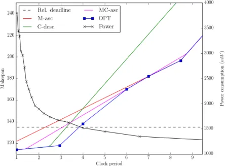
In order to exemplify how the proposed algorithm can be used to optimize the power consumption, we considered a specific task-set consisting of five tasks with the following parameters: τ1 = (24,4), τ2 = (14,2), τ3 = (2,4), τ4 = (60,10),
τ5= (12,3). The relative deadline of the task-set isD= 135. To determine the operating frequency of the CPU, we compared our optimal algorithm, referred to as OPT, against three simple heuristic scheduling strategies:
• M-asc: tasks are scheduled by ascending values ofMi;
• C-desc: tasks are scheduled by descending values ofCi;
• MC-asc: tasks are scheduled by ascending values ofMi/Ci.
Figure 5 shows how the makespan varies according to the scheduling strategies compared. The adopted power model is also reported in the same figure. The optimal operating frequency of the CPU can be identified as the value of clock period where the functionOP T intersects the horizontal line corresponding to the relative deadline of the task-set, i.e.,Tck= 3.842. According
to our power model, such a value corresponds to a power consumption of about 1520 mW. Instead, the heuristic scheduling strategies identify a much lower clock period values for the CPU (3.27for C-desc,3.08 for MC-asc,2.3 for M-asc), which correspond to a higher power consumption (1614mW,1636mW, and 1760mW, respectively).
Fig. 5. Example of a task-set composed of five tasks with parametersτ1= (24,4),τ2= (14,2),τ3= (2,4),τ4= (60,10),τ5 = (12,3)and relative
deadlineD= 135.
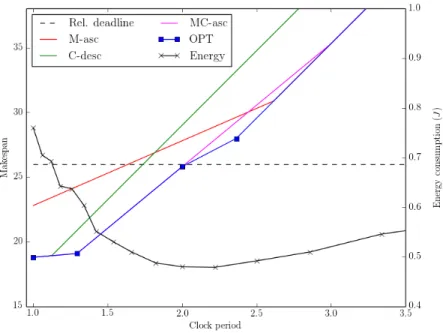
The performance benefit of our algorithm is also evident whenever the energy consumption is the parameter to be optimized. Consider an example task-set consisting of five tasks with D = 26 and the following parameters: τ1 = (4,2),τ2 = (4,1),
τ3 = (8,2), τ4 = (6,5), τ5 = (3,1.5). In our model the energy consumption has a convex shape, and reaches its global minimum (0.48 J) in correspondence ofTck ≈2 (see Figure 6). For this value, the task-set is schedulable according to our
optimal scheduling strategy, and also by MC-asc, as the two functions coincide until Tck = 2. However, the other heuristic
solutions do not allow selecting the optimal operating frequency, because that value would render the task-set unschedulable. Hence, M-asc andC-desc would require to select a lower value of clock period (1.75and1.66, respectively), determining a much larger energy consumption.
Finally, we performed an extensive simulation experiment to quantify the schedulability advantage that can be gained if an optimal scheduling strategy is adopted with respect to the heuristic approaches mentioned above. In particular, we generated
10000 task-sets in total; for each of them, the number of tasks is chosen in the interval n∈[2,10]. The task parameters are then selected as follows: first, Ci is uniformly chosen in[1,10], and then Mi is selected in the interval[Ci, Ci·50] (in this
way, we ensure that, for Tck= 1, computation times are smaller than the respective memory-access times, which represents
the most general configuration). By varying the clock period Tck in the interval [1,20], we measured for each value Tck=t
its average schedulability advantage, defined as the average ratio
Pn i=1Mi+t·P n i=1Ci µalgt ,
Fig. 6. Example of a task-set composed of five tasks with parametersτ1= (4,2),τ2= (4,1),τ3= (8,2),τ4= (6,5),τ5= (3,1.5)and relative deadline
D= 26.
where µalgt represents the value of the makespan at Tck = t when alg is the adopted scheduling strategy. Intuitively, this
quantity represents how much the considered scheduling strategy is able to gain over a sequential execution. The results are shown in Figure 7. As expected, the curve corresponding to OPT dominates the other ones. The schedulability advantage of
OP T is much more evident for larger values ofTck, where all heuristic strategies show a significant performance degradation.
Notably, the performance ofC-descexhibits the worst performance, since for large value ofTckthe optimal ordering is achieved
by ordering the jobs at increasing values ofMi.
Fig. 7. Average schedulability advantage of the optimal scheduling strategy in comparison to heuristic approaches.
VIII. CONCLUSION ANDFUTUREWORK
Co-scheduling algorithms are increasingly being developed to exploit the great potential of modern architectures, and particularly to coordinate the access to memory and computing resources. In this paper, we considered a system composed of DMA-CPU tasks executing sequentially on the two resources. We developed an algorithm that optimally determines the speed of either resource as the one that minimizes power consumption while ensuring the schedulability of the considered task-set.
The algorithm leverages the seminal results on flow-shop scheduling to propose an exact solution for the problem. In addition, the algorithm is shown to have a quadratic complexity in the task-set size, hence it can be efficiently applied for both offline and online operations.
As future work, we plan to extend our results by considering simultaneous variations in the speed of the two resources. We also intend to apply our approach to three-stage task systems in special sub-cases of interest, widening its applicability to more general task models. Finally, we envision that by introducing additional assumptions or constraints to the problem, the time complexity of our algorithm could be further improved.
ACKNOWLEDGMENT
The material presented in this paper is based upon work supported by the National Science Foundation (NSF) under grant numbers CNS-1035736, CNS-1219064, and CNS-1302563. Any opinions, findings, and conclusions or recommendations expressed in this publication are those of the authors and do not necessarily reflect the views of the NSF.
REFERENCES
[1] R. Pellizzoni, E. Betti, S. Bak, G. Yao, J. Criswell, M. Caccamo, and R. Kegley. A predictable execution model for COTS-based embedded systems. In17th IEEE Real-Time and Embedded Technology and Applications Symposium (RTAS), April 2011.
[2] G. Yao, R. Pellizzoni, S. Bak, E. Betti, and M. Caccamo. Memory-centric scheduling for multicore hard real-time systems. In Real-Time Systems. Springer, 2011.
[3] M.R. Garey, D.S. Johnson, and R. Sethi. The complexity of flowshop and jobshop scheduling.Mathematics of Operation Research, 1(2):117–129, 1976. [4] S.M. Johnson. Optimal two- and three-stage production schedules with setup times included. Naval Res. Logist. Q., 1:61–68, 1954.
[5] J.A. Hoogeveen, J.K. Lenstra, and B. Veltman. Preemptive scheduling in a two-stage multiprocessor shop is NP-hard. European J. Oper. Res., 89: 172–175, 1996.
[6] B. Chen. Analysis of classes of heuristics for scheduling a two-stage flow shop with parallel machines at one stage.Journal of the Operational Research Society, 46(2):234–244, 1995.
[7] P. Schuurman and G. J. Woeginger. A polynomial time approximation scheme for the two-stage multiprocessor flow shop problem.Theor. Comput. Sci., 237(1-2):105–122, 2000.
[8] A. Alhammad and R. Pellizzoni. Schedulability analysis of global memory-predictable scheduling. In14th International Conference on Embedded Software (EMSOFT), October 2014.
[9] A. Alhammad, S. Wasly, and R. Pellizzoni. Memory efficient global scheduling of real-time tasks. In21st IEEE Real-Time and Embedded Technology and Applications Symposium (RTAS), April 2015.
[10] A. Melani, M. Bertogna, V. Bonifaci, A. Marchetti-Spaccamela, and G. Buttazzo. Memory-processor co-scheduling in fixed priority systems. In23rd International Conference on Real-Time Networks and Systems (RTNS), November 2015.
[11] B. Egger, J. Lee, and H. Shin. Scratchpad memory management in a multitasking environment. In8th ACM International Conference on Embedded Software (EMSOFT), October 2008.
[12] S. Wasly and R. Pellizzoni. A dynamic scratchpad memory unit for predictable real-time embedded systems. In25th Euromicro Conference on Real-Time Systems (ECRTS), July 2013.
[13] S. Wasly and R. Pellizzoni. Hiding memory latency using fixed priority scheduling. In20th IEEE Real-Time and Embedded Technology and Applications Symposium (RTAS), April 2014.
[14] J. M. Rabaey, A. Chandrakasan, and B. Nikolic. Digital Integrated Circuits (2nd Edition). Prentice Hall electronics and VLSI series. Prentice Hall, January 2003. ISBN 0130909963.
[15] S.K. Venkata, I. Ahn, Donghwan Jeon, A. Gupta, C. Louie, S. Garcia, S. Belongie, and M.B. Taylor. SD-VBS: The San Diego Vision Benchmark Suite. InWorkload Characterization, 2009. IISWC 2009. IEEE International Symposium on, pages 55–64, Oct 2009.
[16] K. De Vogeleer, G. Memmi, P. Jouvelot, and F. Coelho. The energy/frequency convexity rule: Modeling and experimental validation on mobile devices. InParallel Processing and Applied Mathematics, volume 8384 ofLecture Notes in Computer Science, pages 793–803. Springer, 2014.