DESIGN AND OPTIMIZATION OF ELECTRICALLY SMALL ANTENNAS FOR HIGH FREQUENCY (HF) APPLICATIONS

DESIGN AND OPTIMIZATION OF ELECTRICALLY SMALL ANTENNAS FOR HIGH FREQUENCY (HF) APPLICATIONS

A DISSERTATION SUBMITTED TO THE GRADUATE DIVISION OF THE UNIVERSITY OF HAWAI‘I AT MĀNOA IN PARTIAL FULFILLMENT OF THE

REQUIREMENTS FOR THE DEGREE OF DOCTOR OF PHILOSOPHY IN ELECTRICAL ENGINEERING DECEMBER 2014 By James M. Baker Dissertation Committee: Magdy F. Iskander, Chairperson

Zhengqing Yun David Garmire Victor Lubecke John Madey

Copyright By James M. Baker

2014

ABSTRACT

This dissertation presents new concepts and design approaches for the development and optimization of electrically small antennas (ESA) suitable for high frequency (HF) radio communications and coastal surface wave radar applications. For many ESA

applications, the primary characteristics of interest (and limiting factors) are lowest self-resonant frequency achieved, input impedance, radiation resistance, and maximum bandwidth achieved. The trade-offs between these characteristics must be balanced when reducing antenna size in order to retain acceptable performance. The concept of “inner toploading” is introduced and utilized in traditional and new designs to reduce antenna ka and resonant frequencies without increasing physical size. Two different design

approaches for implementing the new concept were pursued and results presented. The first design approach investigated toroidal and helical designs, including combinations of toroidal helical antennas, helical meandering line antennas, and additional designs

incorporating toploading and folding to improve performance. The other approach investigated fractal-based designs in two and three dimensions to improve performance, reduce size, and lower resonant frequency. The performance characteristics of fractal geometries were analyzed and compared with non-fractal designs of similar height, total wire length, and ka. Inner toploading was also applied in the two design approaches and shown to reduce antenna Q by up to a factor of 4 with a corresponding increase in input resistance by up to a factor of 10, when properly applied. When folded arms were applied to various designs, Q was further decreased by a factor of 2 with a corresponding increase in input resistance proportional to the number of arms. Genetic algorithms were

developed for optimizing antenna designs and used in custom programs, including a new iii

cost function for better comparison of ESA performance. Antenna performance was modeled, analyzed, and optimized using set performance criteria. Several unique antenna designs were simulated and experimentally tested in field measurements.

Experimentation was conducted using full-size prototypes with performance measured using vector network analyzers and HF transceivers. Experimental performance

measurements were reproduced in simulation models with a high degree of correlation. Successful two-way radio communications were established with amateur radio stations around the world using prototype antennas.

TABLE

OF CONTENTS

ABSTRACT ... iii

LIST OF TABLES ...vii

LIST OF FIGURES ... viii

ACRONYMS ...xii

CHAPTER 1 INTRODUCTION ... 1

A. BACKGROUND ... 1

B. OBJECTIVE ... 3

C. ORGANIZATION... 4

CHAPTER 2 ELECTRICALLY SMALL ANTENNAS... 6

A. BACKGROUND ... 6

B. PROPERTIES ... 7

C. DESIGN PRINCIPLES ... 14

CHAPTER 3 METHODS OF SOLUTION ... 17

A. NUMERICAL ELECTROMAGNETICS CODE (NEC) ... 17

B. LABVIEW ... 18

C. FEKO ... 20

CHAPTER 4 EVALUATION OF ESTABLISHED DESIGNS AND METHODS ... 21

A. ESTABLISHED DESIGNS ... 21

B. TOPLOADING ... 23

C. FOLDING ... 28

D. SUMMARY ... 31

CHAPTER 5 NEW CONCEPT AND DESIGN APPROACHES ... 32

A. BACKGROUND ... 32

B. INNER TOPLOADING... 33

C. NEW DESIGN METHODOLOGY ... 38

D. NOVEL DESIGNS FOR ELECTRICALLY SMALL HFANTENNAS ... 39

E. INVESTIGATION OF FRACTAL GEOMETRIES ... 53

F. SUMMARY ... 72

CHAPTER 6 ALGORITHMS FOR DESIGN OPTIMIZATION ... 74

A. RANDOM SEARCH ... 74

B. NELDER-MEAD DOWNHILL SIMPLEX ALGORITHM ... 74

C. SIMULATED ANNEALING (SA) ... 75

D. GENETIC ALGORITHMS (GA) ... 75

E. SUMMARY ... 83

CHAPTER 7 EXPERIMENTAL VERIFICATION ... 84

A. FIELD TEST CONFIGURATIONS ... 84

B. FIELD MEASUREMENTS ... 85

CHAPTER 8 SUMMARY AND CONCLUSIONS ... 98

CHAPTER 9 FUTURE WORK ... 101

REFERENCES ... 102 APPENDIX A – ENGLISH TRANSLATION OF HILBERT (1891) ...A-1 APPENDIX B – FRACTAL GEOMETRY ... B-1

List of Tables

Table 1. Shortened Monopole Performance ... 14

Table 2. Toploaded λ/4 Monopole Performance ... 25

Table 3. MLA Performance ... 30

Table 4. Design Analysis for Inner Toploading... 34

Table 5. Helical MLA Performance... 41

Table 6. Performance for three-arm HMLA, direction of helical coils modified ... 45

Table 7. Helical MLA and Toroidal Helical Performance ... 52

Table 8. Fractal Tree Performance at 20 MHz, one meter height ... 63

Table 9. Fractal Tree and Helical Fractal Tree Performance ... 66

Table 10. Hilbert Curve Simulated Performance ... 70

Table 11. Baseline and GA Optimized Performance ... 80

List of Figures

Figure 1: Landing Craft Air Cushion (LCAC) ... 2

Figure 2: Normalized wave resistance ... 12

Figure 3: Normalized wave reactance ... 12

Figure 4: Current distribution for λ/4, λ/8, and λ/20 monopole antennas ... 15

Figure 5: Chu and Hansen/Collin limits with shortened monopoles from Table 1 ... 16

Figure 6: LabVIEW program for Genetic Algorithms ... 19

Figure 7: LabVIEW program for controlling HP8753B Network Analyzer ... 19

Figure 8: FEKO display for early ESA prototype ... 20

Figure 9: Performance of established designs, Q(ka) ... 22

Figure 10: NEC model of Marconi’s 1904 toploaded antenna ... 23

Figure 11: Monopole antenna over PEC ground (left) and with mesh toploading (right)25 Figure 12: Current distribution for monopole with and without toploading ... 26

Figure 13: Two-arm and three-arm folded monopole antennas ... 29

Figure 14: Folded meandering line antenna with three arms ... 30

Figure 15: The concept of inner toploading ... 33

Figure 16: One-turn helical with inner toploading. ... 35

Figure 17: Current Magnitude, helical antenna with and without inner toploading. ... 35

Figure 18: One-turn helical with inner toploading. ... 36

Figure 20: Simulated and measured S11with and without inner toploading ... 37

Figure 19: Prototype helical antenna with inner toploading ... 37

Figure 21: Helical meandering line antenna ... 39

Figure 22: Impedance, helical MLA, 3 – 30 MHz ... 40 viii

Figure 23: Impedance, helical MLA, 30 – 100 MHz ... 40

Figure 24: Far-field radiation pattern ... 42

Figure 25: Current magnitude in three-arm helical MLA ... 43

Figure 26: Current Magnitude in one arm ... 44

Figure 27: Current Phase in one arm ... 44

Figure 28: HMLA single arm, original (left), modified with alternating turns (right) .... 45

Figure 29: One-turn toroidal helical antenna ... 46

Figure 30: Impedance for one-turn toroidal helical antenna ... 47

Figure 31: Gain for one-turn toroidal helical antenna ... 47

Figure 32: One-turn toroidal helical antenna with two-turn inner toploading ... 48

Figure 33: Impedance for one-turn toroidal helical antenna with inner toploading ... 49

Figure 34: Gain for one-turn toroidal helical antenna with inner toploading ... 49

Figure 35: Toroidal helical antenna with four half-turn folded arms ... 50

Figure 36: Impedance for half-turn toroidal helical antenna, four folded arms... 51

Figure 37: Gain for half-turn toroidal helical antenna, four folded arms ... 51

Figure 38: Generator for a Koch curve ... 54

Figure 39: Koch antennas after one and two iterations ... 54

Figure 40: Sierpinski Triangle from IFS ... 55

Figure 41: Fractal tree from IFS ... 55

Figure 42: Fractal tree antennas, iteration #2 and #3 ... 56

Figure 43: Fractal tree antenna with two arms, iteration #4 ... 57

Figure 44: Fractal tree antenna with three arms, iteration #4 ... 58

Figure 45: Fractal tree antenna with four arms, iteration #4... 59

Figure 46: Helical fractal tree with two arms, iteration #1 ... 60

Figure 47: Helical fractal tree with two arms, iteration #2 ... 61

Figure 48: Comparison of fractal tree geometries ... 62

Figure 49: Impedance for four-arm fractal tree ... 64

Figure 50: Current Magnitude for four-arm fractal tree ... 64

Figure 51: Gain pattern for four-arm fractal tree ... 65

Figure 52: Hilbert curves ... 67

Figure 53: Antenna, Hilbert curve, one iteration ... 68

Figure 54: Antenna, Hilbert curve, second iteration ... 69

Figure 55: Antenna Prototype, Hilbert curve, second iteration ... 70

Figure 56: Simulated and measured S11 for Hilbert prototype ... 71

Figure 57: Simulated and measured Impedance for Hilbert prototype ... 71

Figure 58: GA optimized model ... 79

Figure 59: Q and input resistance for four-arm GA ... 80

Figure 60: Impedance, baseline design ... 81

Figure 61: Impedance, GA optimized design ... 81

Figure 62: Improvement in Q ... 82

Figure 63: Improvement in effective radius... 82

Figure 64: Simulated and measured S11, open circuit mode over lossy ground ... 87

Figure 65: Simulated and measured S11, short circuit mode over lossy ground ... 87

Figure 66: Simulated and measured HPBW ... 88

Figure 67: Measuring antenna patterns near Hanauma Bay ... 89

Figure 68: Received power measured over azimuth ... 90

Figure 69: Simulated and measured gain at 16 MHz ... 90

Figure 70: Smith chart of measured impedance, open circuit mode... 91

Figure 71: Smith chart of measured impedance, short circuit mode ... 92

Figure 72: Field testing on beach near the Makai Research Pier ... 93

Figure 73: Amateur Radio Communications – Field Testing ... 94

Figure 74: Measuring two-element array properties at Waimanalo Park ... 95

Figure 75: Power Spectral Density, with and without filtering ... 96

Figure 76: Field testing at Sandy Beach ... 97

Figure 77: Q(ka) in this dissertation ... 100 Figure 78: Hilbert (1891) Figs. 1, 2, and 3 ... A-2 Figure 79: Riemann cosine function R(t) for n = 1 ... B-2 Figure 80: Riemann cosine function R(t) for n = 5 ... B-2 Figure 81: Riemann cosine function R(t) for n = 200 ... B-2 Figure 82: Riemann R(x,y) cosine function ... B-2 Figure 83: Riemann R(x,y) sine function ... B-2 Figure 84: Riemann function 0 to pi ... B-2 Figure 85: Scaling the Riemann function ... B-2

Acronyms

CW Continuous Wave

ηr Radiation Efficiency ESA Electrically Small Antenna

GA Genetic Algorithms

HCAC Hawaii Center for Advanced Communications

HF High Frequency (3 - 30 MHz)

HFSWR High Frequency Surface Wave Radar

HP Hewlett-Packard

hn Spherical Hankel function of the second kind for mode n

HPBW Half-power Bandwidth

IFS Iterated Function System (applies to fractal generation) LCAC Landing Craft Air Cushion

MLA Meandering Line Antenna

MoM Method of Moments

NEC Numerical Electromagnetics Code PEC Perfect Electric Conductor

Q Radiation Quality Factor

RF Radio Frequency

RLC Resistor, Inductor, and Capacitor

RPF Radiation Power Factor

TE Transverse Electric mode

TM Transverse Magnetic mode

UHF Ultra High Frequency (300 MHz - 3 GHz) VHF Very High Frequency (30 - 300 MHz)

VNA Vector Network Analyzer

VSWR Voltage Standing Wave Ratio

Chapter 1

Introduction

A.

Background

The design of electrically small antennas (ESA) presents a wide variety of challenges, primarily due to inherently low impedance and narrow bandwidths. Improving these performance characteristics is especially challenging in the HF band (3 – 30 MHz) due to the longer wavelengths (10 – 100 meters) and corresponding antenna physical

dimensions. These challenges are amplified for applications such as coastal HF surface wave radar (HFSWR) systems which also require vertical polarization for long range surface wave propagation over the ocean, and military applications that require mobile, rapidly deployable, covert systems.

A typical coastal HFSWR antenna system involves arrays of quarter-wave monopole structures with antenna heights of up to 25 meters and even larger ground radial

networks. As a result, current HFSWR and over the horizon radar (OTHR) antenna systems tend to be located at fixed sites with extensive infrastructure and site preparation requirements. These radar arrays can extend for several kilometers with semi-permanent structures and significant environmental impact. Many current systems use quarter-wave monopole antennas which are omnidirectional, requiring extensive arrays to accomplish the beam-forming required to minimize clutter and back-scatter from the surrounding terrain. Coastal HF radar system performance is also affected by ionospheric conditions which are constantly changing and impact the useable frequencies available. These systems may operate as intended in the geographic region in which they are constructed, but are not suitable for mobile operations or rapid deployment to remote, desolate, or

otherwise unprepared locations. For these types of applications, the primary characteristics of interest (and limiting factors) in antenna design are self-resonant frequencies, impedance, gain, bandwidth, polarization, and phase stability. For military and homeland security applications, the antenna may also be required to consist of a low or otherwise compact physical profile to camouflage its purpose. However, disguising a 25 meter high antenna without limiting performance or mobility can be challenging. The implementation of HF radios on military mobile platforms is also problematic with the antenna size being restricted by operational factors such vehicle size, tactical profile requirements, or logistical issues. In Naval applications, traditional HF antennas can also be an issue due to size and space limitations on seaworthy platforms such as the Landing Craft Air Cushion (LCAC). The current HF antenna installed on the LCAC is a

horizontal center-fed dipole, aligned longitudinally with the vessel, mounted just a few feet above the metal structure. This antenna configuration is roughly depicted by the solid black line in Figure 1.

Figure 1: Landing Craft Air Cushion (LCAC) 2

The reality remains though that many LCAC radio operators rely on VHF and UHF radio systems because the HF communications are unreliable. This is one of many examples of the need for a low-profile HF antenna system that retains acceptable radio frequency (RF) performance while satisfying non-RF design requirements. An additional consideration for practical applications is the requirement for low-profile antennas to exhibit broadband or multi-resonance characteristics to support system operations at different frequencies as atmospheric and other propagation conditions change. For these and other HF systems (particularly those suitable for mobile surveillance,

communications, and homeland security applications) antenna size is considered a critical factor. Clearly, there is still room for improvement in traditional HF antenna design and the requirement remains for compact, low profile HF antenna designs that are suitable for mobile, tactical, and other mission-specific applications.

B.

Objective

The objective for this research was to find solutions to the current challenges and limitations in designing electrically small antennas in the HF band for homeland security and military applications through the investigation of new design methodologies and approaches. This dissertation presents a new design methodology that represents a

paradigm shift from traditional and currently accepted practices. Two different innovative antenna design approaches, developed using the new methodology, are presented.

The specific tasks identified for this effort were:

1) study established designs and review their characteristics and limitations

2) explore new avenues for more effectively utilizing an antenna’s enclosed volume 3) explore methods for design optimization

4) select promising designs and build prototypes for field experimentation The desired outcomes include a study of the trade-offs involved in performance optimization, producing new and functional designs for HF ESA, and validation of predicted performance through field experimentation with full-size antenna prototypes.

C.

Organization

Chapter 2 provides a review of the fundamental characteristics and limitations of electrically small antennas. These fundamental characteristics are used to develop consistent and practical measures and metrics for comparing antenna performance, regardless of specific physical features. Chapter 3 presents an overview of the tools and methods used for developing solutions and analyzing results. The primary tools used were Numerical Electromagnetics Code (NEC) and National Instruments LabVIEW application development environment. Several custom applications were specifically developed which integrated NEC and LabVIEW into single applications for the automation of design and analysis. LabVIEW was primarily used to develop user interfaces for auto-generating antenna designs based on user input (e.g., designs

generated using genetic algorithms) and NEC was used to simulate antenna designs and provide performance data for further analysis. FEKO was also used for simulating

various antenna designs during the early phases of research. Chapter 4 reviews traditional

ESA antenna designs along with methods for improving performance, specifically the effects of toploading and folding when applied to canonical geometries. Benefits and trade-offs for each design methodology are evaluated and compared. Chapters 5 presents a new design methodology for optimizing antenna geometries to better utilize the inner volume along with two design approaches for implementing the new concept. The first design approach examines toroidal and helical designs which utilize their total inner volume. Innovative designs and geometries were developed using this design approach. Designs presented include helical meandering line antenna (MLA) geometries, designs combining toroidal and helical elements, and fractal geometries. Fractal geometries are reviewed with the focus on Hilbert curves and fractal tree and helical fractal tree designs. Computer applications were developed to generate fractal images for use in antenna design and performance analysis, and for evaluating the benefits of this approach. These antennas were designed to explore different methods (e.g., inner toploading) for using their inner space to reduce total antenna volume and achieve lower resonant frequencies. Chapter 6 investigates various techniques for performance optimization using methods such as random search, simulated annealing, and genetic algorithms. The chapter finishes with a comprehensive investigation into the use of genetic algorithms for optimizing a helical MLA design. Chapter 7 describes the extensive field testing conducted using full-size antenna prototypes and provides detailed results and design comparisons. Chapter 8 provides a summary of observations and conclusions developed throughout this research effort. Chapter 9 describes areas of opportunity for future work building on the designs and concepts presented.

Chapter 2

Electrically Small Antennas

A.

Background

Over the years there have been many contributors to the theory and design of antennas that are considered electrically small. Wheeler [1] [2] and Chu [3] pioneered the field by developing fundamental properties of electrically small antennas. The generally accepted criteria for what makes an antenna “electrically small” is based on the spherical volume occupied by the antenna. Using the free-space wave number k = 2π/λ and the radius a of the sphere enclosing an antenna, it is considered to be electrically small when the value of ka is less than or equal to 0.5 [4]. In the early days of radio communications all antennas were electrically small. Hansen provides a chronology of electrically small antennas beginning in 1889 with the Hertz loop antenna, followed by Marconi’s long wire antennas [5].

It is important to identify the relevant metrics for meaningful comparison of various dissimilar antenna geometries. The following sections review fundamental and practical performance properties that have been well-established for antennas in general, the fundamental limitations to these properties for electrically small antennas, and the derivation of practical metrics for characterizing performance of antenna geometries. This is necessary to provide for consistent and practical analysis and comparison for all designs presented herein, as well as any other published designs, regardless of specific geometry.

B.

Properties

1) Wheeler’s Radiation Power Factor

Wheeler [1] developed radiation power factor (RPF) as a figure of merit for electrically small antennas, provided here for electric (1) and magnetic (2) antennas.

Wheeler also developed the concept of a radian sphere: a sphere with radius equal to one radian length (r = λ/2π). The radian sphere defines the transition between the near- field and far-field regions of an electrically small antenna [2]. The radian sphere is used to determine the effective antenna volume and its associated effective radius. The volume of the radian sphere and the equivalent radian cube is stated in (3).

From this expression and the RPF, represented by p, the effective antenna volume can be calculated (4). 3 2 3

3

4

λ

π

ω

b

a

C

G

p

=

=

3

4

λ

π

ω

b

a

L

R

p

=

=

V

π

π

λ

π

V

3

4

2

3

4

=













=

p

V

p

V

V

2

9

6

=

=

π

From (4), the effective radius can be stated in terms of RPF (5).

This provides a very useful metric for direct comparison of performance improvement for different antenna structures [2]. If the antenna structures being compared are of the same height, the effective radii can be compared directly. If the structures have different heights, the ratio of their respective effective radius to height can be compared.

The constraints developed by Wheeler are considered to be practical rather than fundamental in that they were developed for dipole (electric) and loop (magnetic) antennas [6]. It is also worth noting Wheeler established that the RPF is a function of antenna dimensions and resonant wavelength alone and is the same for electric and magnetic antennas.

2) Chu’s limit on Q

Chu derived a radiation quality factor (Q) for a hypothetical antenna enclosed in a sphere of radius a. The electromagnetic fields outside the sphere could be described in terms of infinite series of transverse electric (TE) and transverse magnetic (TM) modes. Chu defined Q at the input terminals of an antenna structure based on its equivalent RLC circuit and expressed as a function of the energy stored beyond the input terminals and the power dissipated in radiation [3]. Chu expanded the mode wave impedance into a continued fraction that could be interpreted as a ladder network of capacitors and inductors. This minimum Q is considered to be a fundamental limitation for electrically small antennas because it applies to any antenna configuration that fits within a sphere of

3 1

2

9

2













=

p

r

π

λ

radius a and excites a single TM mode [3]. This fundamental limit was later re-examined by McLean [7] who derived an expression for Q based on antenna ka (6). Chu’s Q did not include stored energy inside the sphere and so is considered the lower bound for

lossless antennas. Many papers over the years have refined and modified this expression to increase the value for predicted Q in search of better agreement with measured antenna performance. One estimate for Q was developed by Hansen and Collin [6] using numeric methods and curve fitting to better predict measured performance for the lowest order TM mode as depicted in (7). This approximation was said to be accurate within 0.5%

for ka ranging from 0.1 to 0.5 and is useful when comparing simulation results for loss-less antennas in free space or over PEC ground planes. More recent publications continue to refer to (6) while adding an efficiency term as shown in (8), where ηr represents radiation efficiency [8].

( )

2

3

)

(

2

1

a

k

a

k

Q

=

+

( )













+

=

ka

ka

Q

η

1

1

( )

ka

ka

Q

=

1

+

1

Wheeler’s RPF has been shown to be related to Chu’s Q as p = 1/Q and so the effective radius (5) can be re-expressed in terms of Q (9).

Yaghjian and Best developed an expression (10) for Q derived directly from antenna impedance and radian frequency [9] which provides an additional metric, independent of ka, for comparing the quality factor of different antenna geometries.

This approximation of Qz(ω), with R'(ωo) and X'(ωo) representing the derivative of the resistance and reactance with respect to the radian frequency (ω), is valid for antennas with a single resonance within the resonant bandwidth. This expression can be calculated and analyzed over ranges including anti-resonant as well as resonant frequencies [8]. It also provides an additional parameter for comparing antenna performance between designs with differing geometries and dimensions as well as for comparing performance of a specific design to fundamental limitations.

( )

( )

( )

( )

( )

2













+

′

+

′

=

ω

ω

ω

ω

ω

ω

ω

R

X

X

R

Q

2

9

2













=

Q

r

π

λ

3) Wave impedance

Chu defined voltage (11), current (12), and impedance (13) of an equivalent circuit for the spherical waves outside the radian sphere for the TMn mode [3], where hn is the spherical Hankel function of the second kind for mode n, permeability µο and permittivity εο for free space, and ρ = ka.

Harrington further expanded these definitions for the TEn modes [10], showing that

impedance for the TEn mode is equal to the admittance of the TMn mode (14).

These equations for TE and TM mode impedances are significant as they are only dependent on the ka of an antenna’s geometry and they represent the normalized impedances of the spherical waves that will couple to free space for far-field radiation. The resistive component of the TMn mode (normalized) is presented in Figure 2 where a

significant decrease in resistance is readily observed as the value of ka is decreased from

( )

ρ

ρ

ρ

π

ε

µ

d

h

d

j

n

n

n

k

A

V

1

2

)

1

(

4













+

+













=

)

(

1

2

)

1

(

4

ρ

ρ

π

ε

µ

h

n

n

n

k

A

I













+

+













=

( )

)

(

/

ρ

ρ

ρ

ρ

ρ

h

d

h

d

j

Z

=

( )

ρ

ρ

ρ

ρ

ρ

d

h

d

j

h

Z

=

(

)

/

0.5 down towards 0.0. It is also observed that for ka < 0.5 only the first mode has any useable resistance for supporting propagation. The normalized reactive component of wave impedance is plotted in Figure 3 where the negative reactance increases (in

magnitude) significantly as ka is decreased below 0.5. For comparison purposes the ka of a quarter-wave monopole, ka ≈ 1.5, is also depicted in the two figures.

Figure 2: Normalized wave resistance

Figure 3: Normalized wave reactance 12

4) Radiation Resistance

The term “radiation resistance” is defined in the IEEE Standard Definition of Terms for Antennas (IEEE Std 145-1993) as “the ratio of the power radiated by an antenna to the square of the RMS antenna current referred to a specified point”. In the general case for arbitrary current distribution on a lossless dipole, radiated power [11] can be expressed in terms of average current amplitude and antenna length, as shown in (15), where β = 2π/λ, and L = antenna length [12].

Radiation resistance for an electrically small dipole antenna can then be expressed (16) in terms of the ratio of average to peak current and the ratio of physical length to

wavelength (Lλ = L/λ) [12].

This approximation is valid for antennas with L << λ. Antennas with dimension ka < 0.5 (equivalently, Lλ < .08) easily satisfy this limitation.

5) Effects of Height, Volume, and Wire Length

The antenna radiation resistance is proportional to (L/λ)2, therefore wire antennas of the same height and resonant frequency generally exhibit the same properties, independent of their geometries. Lower resonant frequencies can be achieved when the geometry

effectively utilizes available height and overall volume to meet design goals and

(15) (16)

π

β

ε

µ

12

L

I

P

=

790

L

I

I

R













≅

requirements. The challenge is to minimize the impact on performance when reducing the height or volume. The length of the wire inside the antenna volume is the dominant factor in establishing resonant frequency. For folded arm geometries, the wire length of one arm is used to determine the wavelength of the resonant frequency because the current

distribution is symmetrical in all the arms. Increasing wire length is one way to increase antenna inductance, but may also decrease the resonant frequency if done

indiscriminately. Decreasing the wire diameter is one method for decreasing the resonant frequency; this will reduce the antenna’s radiation efficiency, which may or may not be an acceptable trade-off.

C.

Design Principles

In order to capture the impact of the limitations on performance for electrically small antennas, a simple quarter-wave (λ/4) monopole was designed for resonance at 6 MHz. The wire length was progressively reduced from λ/4 down to λ/20 with the impacts on performance analyzed, compared, and results reported in Table 1, where r’/h represents the effective radius normalized by the physical height. This metric provides a useful parameter for comparing performance changes between antennas independent of specific geometries.

Table 1. Shortened Monopole Performance

Antenna ka Height (meters) Resistance (Ω) Reactance (Ω) Qz(ω) r’/h λ/4 1.49 11.8 36.0 0 6.4 0.60 λ/8 0.75 5.9 6.5 -249 50.2 0.60 λ/10 0.60 4.7 3.9 -322 95.5 0.60 λ/12 0.496 4.0 2.7 -385 160.0 0.61 λ/20 0.298 2.4 0.9 -580 657.9 0.63 14

This preliminary analysis demonstrated the unavoidable impact on performance characteristics as the length of a lossless monopole over PEC ground plane was reduced. The geometries were modeled in NEC version 4.2 [13] using 15 segments to calculate the distribution of electric current. The current distributions for λ/4, λ/8, and λ/20

configurations were calculated at the center of each segment and are plotted in Figure 4. It can be seen from Table 1 that for a simple monopole antenna to be considered

“electrically small” its height must be ~λ/12 or less, the radiation resistance is then less than 3Ω, and the Qz(ωο) over 300. The effect of size reduction on antenna current

distribution is apparent in Figure 4 where the sinusoidal distribution for the λ/4 (resonant) antenna quickly converges to a triangular distribution as the height is reduced.

Figure 4: Current distribution for λ/4, λ/8, and λ/20 monopole antennas

0 0.1 0.2 0.3 0.4 0.5 0.6 0.7 0.8 0.9 1 1 2 3 4 5 6 7 8 9 10 11 12 13 14 15 Cu rre nt (a mp s) Segment #

Current Distribution - Monopole

Antennas

one-fourth lambda one-eighth lambda one-twentieth lambda

Specific performance characteristics for the shortened monopole antennas listed in Table 1 are depicted in Figure 5 together with Chu’s limitation and the Hansen/Collin revision to demonstrate the rapid increase in Q as size is reduced. The individual

monopole configurations may be identified in the figure by their ka values from Table 1.

Figure 5: Chu and Hansen/Collin limits with shortened monopoles from Table 1

Chapter 3

Methods of Solution

A.

Numerical Electromagnetics Code (NEC)

The Numerical Electromagnetics Code [13] is a software application used for analyzing the electromagnetic response of antennas and scatterers. It is based on the numerical solution of integral equations using the Method of Moments (MoM), combining electric-field and magnetic-electric-field integral equations for modeling thin wires for closed surfaces. NEC was selected as the engine for modeling and simulating antenna designs because it is optimized for wire and electrically small antennas, and provides command line

executables for 32-bit and 64-bit Windows operating systems. This functionality was used to automate many of the analyses performed as part of the research for this

dissertation, and to facilitate integration with other applications developed in LabVIEW. NEC also supports modeling and simulation using lossy antenna materials and ground planes for comparative analysis with field experimentation data.

The user interface application selected was 4NEC2 version 5.8.14 [14]. This application is available online at no cost and provides an efficient interface to NEC engines for generating properly formatted NEC input files and for graphic analysis of NEC output files. 4NEC2 was used for rapid prototyping and analysis of

three-dimensional wire antenna designs and for analysis of impedance, gain, and electric field components.

When modeling antennas in NEC, it is very important to follow the rules and guidelines published in the NEC User’s Manual [15], especially those related to the relationship between wire radius and segment length. For example, NEC version 4.2 uses a thin-wire

approximation which limits the minimum separation allowed between parallel wires. This recommended minimum separation is two to three times the wire diameter. If parallel wires are placed too closely together errors may be significant, as seen in some published performance results that violate fundamental limits such as Chu’s limit on Q. Model accuracy should be assessed by varying parameters and checking for convergence, and by slightly varying the frequency and observing the sensitivity of the results.

B.

LabVIEW

National Instruments LabVIEW [16] is an advanced graphical programming

environment for developing custom applications in science and engineering. LabVIEW was selected based on its extensive function libraries, instrument driver libraries, and 3D graphing tools which allowed for rapid software prototyping, automated instrument control, and development of comprehensive user interfaces. A wide range of custom software applications were developed in LabVIEW to support the research and analysis efforts in completing this dissertation. These applications ranged from solving and plotting solutions for advanced mathematical equations to controlling external

instrumentation and sensors for test automation, data recording, analysis, and reporting. Specific examples include automated analysis of NEC output files, control and data recording with Anritsu and HP network analyzers, and the implementation of genetic algorithms for antenna optimization. LabVIEW programs were also developed to solve spherical Hankel functions of the second kind for plotting TM and TE mode impedances.

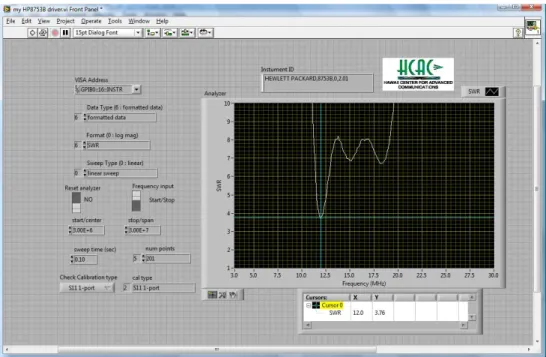
User interfaces for two of the applications developed in LabVIEW are provided below. Figure 6 displays the genetic algorithm application interface including parameters, design goals, and chromosome binary patterns. Figure 7 displays the interface for an HP 8753B network analyzer application, developed for recording and analyzing data during field experimentation.

Figure 7: LabVIEW program for controlling HP8753B Network Analyzer Figure 6: LabVIEW program for Genetic Algorithms

C.

FEKO

FEKO [17] is a commercial application for modeling and simulating complex designs for a variety of applications in electromagnetics. FEKO combines a selection of

numerical methods for analyzing complex structures including antennas, waveguides, and other electromagnetic devices. Numerical methods include Method of Moments, Physical Optics, Geometrical Optics, Uniform Theory of Diffraction, and Finite Element Method. This application is also capable of combining various methods to develop hybrid

solutions.

FEKO was used during the early stages of research for simulation of electrically small antennas, providing insight into design methodology, geometry development, and

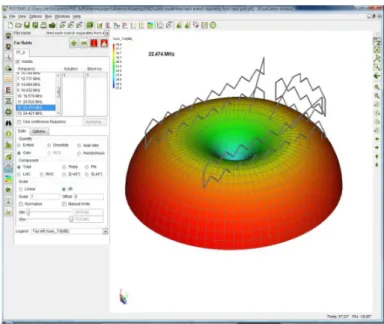
predicted performance characteristics. The graphical analysis products were of very high quality, especially three-dimensional plots of antenna structures combined with far-field radiation patterns. A screenshot is provided in Figure 8 for an early ESA prototype.

Figure 8: FEKO display for early ESA prototype 20

Chapter 4

Evaluation of Established Designs and Methods

A.

Established Designs

Numerous designs were evaluated and compared to determine their limitations and examine potential areas for improving performance, reducing overall size, and achieving multiple resonances and lower frequencies within the HF band. Also examined were two common methods for improving performance: toploading and folding. Designs were selected for inclusion in this review based on several factors:

1) the design was the result of an intentional effort to reduce antenna size or improve performance

2) the design was at least close to meeting the criteria of ka ≤ 0.5

3) the published design performance characteristics had to be reproducible using NEC

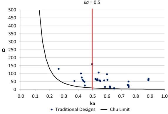
Designs which violated Chu’s fundamental limit or did not provide all the dimensions or other information required for modeling were not included. The designs selected for evaluation are well-documented in [4], [5], [8], [12], [18], [19], and [20], and range from shortened monopoles to multi-arm spherical helical structures. Since most of the

traditional designs considered were developed for VHF and UHF frequencies, their performance was compared by evaluating Q as a function of ka, as depicted in Figure 9.

Two common methods used for reducing antenna size or improving the performance for antenna designs depicted in Figure 9 are toploading and folding. These techniques are well-documented and are discussed here to provide a baseline for expected performance improvements and also to demonstrate how current design methods and approaches restrict the antenna elements to the surface of the enclosed volume or in some cases increase the overall size of the antenna.

Figure 9: Performance of established designs, Q(ka)

B.

Toploading

1) Designs

Toploading is one of the earliest mechanisms employed for reducing the physical size of an HF antenna without giving up too much performance. Marconi described a radial network for reducing the height of vertical HF antennas, documented in his 1904 patent [21]. This antenna design consisted of a reduced height vertical element with a system of 8 radial arms extending outward from the top. Marconi’s design, as modeled in NEC, is depicted in Figure 10.

The purpose of toploading is to modify the current distribution on the vertical (radiating) element from being triangular (as previously depicted in Figure 4) to being more uniform in magnitude along the entire length. As the current distribution is made more uniform, the radiation resistance and corresponding radiated power are also

Figure 10: NEC model of Marconi’s 1904 toploaded antenna

increased. A sampling of toploaded designs described by Best and Hanna [8] were modeled and simulated in NEC to validate the antenna metrics and algorithms implemented herein and to provide a baseline for comparing antenna performance. A comparative analysis of mesh versus radial toploading was conducted to determine the impacts on performance for both structures. The term mesh is used here to describe a web-like wire structure with radial and cross radial components providing multiple symmetric paths for current flow.

The current distribution in a normal mode helical antenna at resonance is similar to other wire antennas, with maximum current at the feed point, zero current at the opposite (open) end of the wire, and continuous distribution along the length of the wire.

Traditional toploading techniques would place a disk or radial network at the top of the helical antenna to provide for more uniform current distribution and for lowering the resonant frequency [8]. The drawbacks of this method include the increase in volume and ka of the antenna due to the additional external components.

2) Simulation Results

NEC models for monopole antennas, with and without mesh toploading, are depicted in Figure 11. These antennas were simulated using a perfect electric conductor (PEC) ground plane; current distribution is represented by color. The NEC simulation results for these two models were comparable to the results in [8] and are listed in Table 2 along with the results for designs scaled to 6 MHz.

Table 2. Toploaded λ/4 Monopole Performance Antenna Frequency (MHz) ka Height (meters) Resistance (Ω) Reactance (Ω) Qz(ω) r’/h Monopole A 300 0.52 .0848 3.0 -461.4 173 0.56 - Mesh 300 0.59 .0848 10.7 0.8 16 1.2 Monopole B 6 0.52 4.22 3.0 -463.7 176 0.56 - Mesh 6 0.59 4.22 10.6 -0.6 16 1.2 - Radial 6 0.63 4.22 10.6 -0.2 16 1.2

Figure 11: Monopole antenna over PEC ground (left) and with mesh toploading (right)

Figure 12 plots the current distribution for a monopole antenna with and without toploading along with a comparison of two different toploading geometries, radial and mesh. The effects of radial and mesh toploading appear to be virtually the same.

The improvement in monopole antenna performance through toploading has been demonstrated. This technique improves performance by providing a more uniform current distribution along the vertical (radiating) element of the antenna due to the relationship between the radiation resistance and the ratio of average to maximum

current, as described earlier in (15) and (16). Given that the ratio of average to maximum current (Iavg/Imax) for a triangular distribution is about 0.5 and the ratio for uniform distribution is about 1.0, the resulting increase for uniform over triangular distribution is 2:1. The radiation resistance is proportional to the square of the current ratio (16) so the

Figure 12: Current distribution for monopole with and without toploading

0 0.1 0.2 0.3 0.4 0.5 0.6 0.7 0.8 0.91 1 2 3 4 5 6 7 8 9 10 11 12 13 14 15 16 17 18 19 20 21 Cu rre nt (A mp s) Segment #

Current Distribution - Monopole Antenna

with and without toploading

Mesh toploading Radial toploading No toploading

maximum achievable improvement in radiation resistance is roughly a factor of four. This property was verified by adding toploading to the design depicted in Figure 11, resulting in an increase of input resistance by a factor of approximately 3.5:1 as observed in Table 2 data. The trade-off however, is an increase in ka resulting from the additional width added by the toploading structure. This may or may not be acceptable depending on the specific design requirements for the antenna physical dimensions.

During the analysis for toploaded designs, two different structures for achieving

uniform current distribution were compared. The radial design depicted in Figure 10 was scaled to the same height as the mesh structure shown in Figure 11 and the width adjusted to achieve self-resonance at 6 MHz. The performance of the radial design was very similar to the results of the mesh structure with the exception of ka which was slightly larger due to the increased radius required to achieve resonance at the same frequency.

C.

Folding

1) Designs

One popular method for increasing the radiation resistance is commonly referred to as “folding” or “folded arms”. The fundamental properties of folding have been well-documented in books and journals including [8], [19], [20], and [22]. The addition of folded elements to a basic antenna is one method for improving the radiation resistance without expanding the height or volume of the antenna. The geometry of a folded antenna typically consists of a symmetrically repeating pattern based on the initial element (e.g., a quarter-wavelength, straight-wire monopole). The additional components are positioned at a specified distance and connected at the ends. The antenna feed point is connected at the base of the initial element while the bases of additional elements are short-circuited to ground. When properly connected, this structure forms a “folded arm” geometry.

Additional arms may be added by short-circuiting the base of the additional elements to ground and connecting all elements to each other at the top. Balanis [19] provides a derivation of the input impedance for folded antennas, which for a simple straight-wire design is proportional to the square of the total number of arms. For example, the input impedance of a quarter-wave monopole antenna (single arm) is about 36 Ω while the input impedance with two folded arms is about 4 times that, or 144 Ω. This property can be very useful when trying to increase input impedance of an electrically small antenna for matching purposes and/or improving radiation performance.

Figure 13 depicts folded monopole antennas with two and three arms, as modeled in NEC. The vertical elements are connected together at the top and connected to the PEC ground at the bottom. The small red circle indicates the feed point.

2) Simulation Results

A variety of folded designs were simulated in NEC with results comparable to

previously published antenna performance. An analysis was conducted on the effects of folding for a meandering line antenna (MLA) [20] designed for resonance at 6 MHz and ka < 0.5. The three arm variant of a folded MLA is depicted in Figure 14 and analysis results for two through six arms are provided in Table 3.

.

Figure 13: Two-arm and three-arm folded monopole antennas

Table 3. MLA Performance # of arms ka Height (meters) Resistance (Ω) Reactance (Ω) Qz(ω) r’/h 2 0.419 2.17 8.5 0.0 100.2 1.29 3 0.424 2.17 17.4 0.0 75.5 1.42 4 0.429 2.17 29.3 0.0 62.2 1.51 5 0.436 2.17 44.6 0.0 54.0 1.59 6 0.443 2.17 63.5 0.0 48.7 1.64

The results listed in Table 3 were obtained through modeling of the design in NEC with #10 copper wire over PEC ground plane. The width of the meandering line component was adjusted for each configuration to maintain resonance at 6 MHz, constant height, and ka < 0.5. The small increases in the width of the meandering elements are reflected in a slight increase in ka.

Figure 14: Folded meandering line antenna with three arms

D.

Summary

The primary benefit of toploading is the uniform current distribution in the radiating elements of the antenna, resulting in a lower resonant frequency. This improvement in the current distribution is realized by providing additional paths for current flow at the end of the monopole element. Different methods for implementing toploading include radial arms, mesh networks, and solid disks, however an important trade-off is the increase in physical size due to the addition of the toploading components.

The value of folded arms is realized in the corresponding increase in input resistance due to the cumulative effects of current distribution in all the arms. The relationship between the number of folded arms and the radiation resistance of an antenna provides a method for optimization of antenna impedance for input matching and improvement of radiation properties. This can be extremely useful for improving the performance of electrically small antennas which typically exhibit input impedances well under 10 Ω. During the evaluation of established designs, it was observed that many designs published as ESA had ka > 0.5 when scaled for the HF frequencies, heights ranged from two to six meters, and many were only resonant at a single frequency in the HF band. It was also observed that a majority of the designs only placed wire on the outer surface of the enclosing volume and many required additional tuning and matching networks. This establishes the need for a new design methodology for electrically small antennas that enables design approaches to effectively utilize the inner volume of an antenna’s geometry.

Chapter 5

New Concept and Design Approaches

A.

Background

A currently prevalent theme in ESA methodologies is that “optimization” involves maximizing the placement of wire on the surface of the sphere enclosing the antenna volume [19]. This section presents a new alternative design methodology utilizing the inner space of the enclosed volume to achieve self-resonances at much lower frequencies. This methodology offers designers an alternative when the design requirements and restrictions on maximum height and volume would otherwise not support self-resonance at a lower required frequency. Several alternative designs have been simulated and analyzed, comparing performance parameters including radiation resistance, Q, bandwidth, and the minimum operating frequency. Results from these simulations are presented and trade-offs discussed. The design approaches presented herein provide innovative methods to utilize the entire volume of the space enclosing the antenna [23], a departure from methods typically described in current publications. The concept of “inner toploading” is introduced here, followed by design approaches for implementing the new concept. Notional requirements were established (for the purposes of this research) for an antenna that is less than one meter high, one meter wide, and resonant within the HF band. The concepts, methodologies, and designs presented herein are targeted for producing an antenna that satisfies those requirements.

B.

Inner Toploading

The concept of inner toploading is a modification of traditional methods by moving the toploading elements from the exterior of the antenna geometry to the interior, as depicted in Figure 15. This provides the toploading effects on current distribution without

increasing the size of the antenna. In this method the radius of the enclosing sphere “a” is kept constant, yet the overall ka is reduced due to the longer wavelengths of the lower resonant frequencies achieved.

The resonant frequency of this design may be tuned by changing the length of the toploading radials inside the volume, similar to traditional toploading. Although helical in nature, the far-field pattern is omnidirectional in azimuth and vertically polarized. A 25% reduction in resonant frequency was achieved in designs using this concept with no increase in antenna enclosed volume.

Figure 15: The concept of inner toploading

Table 4 provides an initial analysis of the effects of inner toploading on the self-resonant frequency, resistance, Qz, and ka for helical antennas with various helical configurations with and without inner toploading. The values provided in Table 4 represent the initial resonance for each design.

Table 4.Design Analysis for Inner Toploading Helical Antenna Parameters Frequency (MHz) Resistance (Ohms) ka Qz Wire Length (meters) Turns: 0.75 26.1 6.917 0.62 44 3.09 Turns: 1.0 21.5 4.572 0.51 67 3.83 Turns: 1.5 15.8 2.674 0.38 123 5.35 Turns: 2.0 12.5 1.864 0.30 187 6.90 Turns: 0.75 with toploading 18.3 4.491 0.43 72 6.19 Turns: 1.0 with toploading 16.0 3.433 0.38 97 6.93 Turns: 1.5 with toploading 12.9 2.381 0.31 152 8.45 Turns: 2.0 with toploading 10.7 1.780 0.26 214 10.0

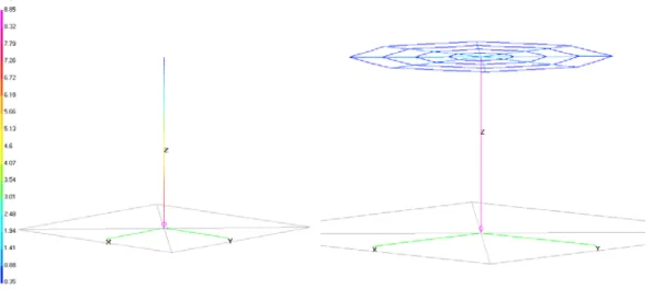
The reduction in self-resonant frequency and the matching reduction in ka were achieved within the same occupied volume due to the improved current distribution provided by the toploading elements. The current magnitude for the one-turn helical antenna depicted in Figure 16 was analyzed with and without inner toploading; results are plotted in Figure 17. This methodology offers designers an alternative when the system design requirements and restrictions on maximum height and volume would otherwise not support self-resonance at a lower (yet required) frequency.

Figure 17: Current Magnitude, helical antenna with and without inner toploading.

0

0.2

0.4

0.6

0.8

1

0

10

20

30

40

50

60

with toploading without toploading

Figure 16: One-turn helical with inner toploading.

The effects of inner toploading on Q as a function of ka for the antenna configurations listed in Table 4 are plotted in Figure 18.

Figure 18: One-turn helical with inner toploading.

0

50

100

150

200

250

0.0

0.1

0.2

0.3

0.4

0.5

0.6

0.7

without toploading with toploading

A prototype two-turn helical antenna was constructed as depicted in Figure 19. A comparison of simulated and measured S11 for the antenna with and without toploading is provided in Figure 20. A frequency reduction of 15% was achieved for this design configuration with no increase in antenna size.

Figure 19: Simulated and measured S11with and without inner toploading -10.0-9.0 -8.0 -7.0 -6.0 -5.0 -4.0 -3.0 -2.0 -1.00.0 140 160 180 200 220 240 260 280 S1 1 Lo g-Mag ( dB ) Frequency (MHz)

without toploading - simulated with toploading - simulated without toploading - measured with toploading - measured Figure 20: Prototype helical antenna with inner toploading

C.

New Design Methodology

There are a variety of methods for adding elements to the surface of an antenna’s enclosed volume to improve performance [8]. In one example, straight wire

components of antenna geometries are replaced with helical components to lower the resonant frequency within a given volume [24]. The methodology and design

approaches presented herein build upon those initial concepts and provide a

framework for more efficient use of the entire volume enclosed by an antenna. This is a departure from methods typically described in current publications which focus on using the outer surface. This methodology is based on first determining any

limitations and requirements for height, volume, and frequency in order to establish the maximum value for ka allowed by those requirements. The preliminary steps required are:

1. Establish the maximum height limitation for the physical antenna 2. Establish the maximum volume limitation for the physical antenna 3. Establish the requirement for lowest operating frequency

4. Determine the ka for the above parameters

5. Determine whether the expected performance for this ka is acceptable (e.g., input impedance and Q)

6. Effectively use the antenna’s inner volume for placing elements in order to achieve required performance (e.g., inner toploading)

Several new design approaches developed using this methodology are presented, including variations on toroidal and helical geometries, helical meandering line geometries, and fractal geometries.

D.

Novel Designs for Electrically Small HF Antennas

1) Helical Meandering Line Antenna (MLA)

A new design combining helical and meandering line elements for compact high

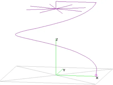
frequency (HF) antennas was presented in [25] and [26]. This antenna was designed to be portable and rapidly deployable, while maintaining a comparatively small profile for mobile radar applications. The Helical MLA design is low-profile (less than one meter high) and provides for effective performance, improved antenna radiation resistance, and strong vertical polarization while maintaining an omnidirectional radiation pattern with low take-off angle. The Helical MLA, depicted in Figure 21, also provides for multiple self-resonance frequencies allowing for selectable channels without requiring additional matching networks.

Figure 21: Helical meandering line antenna 39

Figure 22 depicts the impedance of the helical MLA in the HF band. Figure 23 depicts the impedance for the range 30 – 100 MHz, showing multiple self-resonances above the HF band.

Figure 23: Impedance, helical MLA, 30 – 100 MHz Figure 22: Impedance, helical MLA, 3 – 30 MHz

One of the arms of the helical MLA serves as the input or feed port. The other arms may be either connected to the copper ground disk (folded arm configuration, referred to as the “short” mode) or left open circuit (inner toploading configuration, referred to as the “open” mode). Table 5 provides a comparison of the various effects of number of arms on performance for the helical MLA. This analysis was performed using NEC 4.2 with an infinite PEC ground plane and AWG #10 copper wire. The different effects of toploading (open-circuit mode) versus folding (short-circuit mode) are observed in comparing the performance for various configurations.

Table 5. Helical MLA Performance

# of arms Frequency (MHz) Resistance (Ω) ka Q Efficiency (%) Mode 1 12.20 2.57 0.28 254 63.6 NA 2 13.33 9.97 0.30 154 79.2 SHORT 3 14.47 24.9 0.33 109 86.2 SHORT 4 15.55 49.8 0.35 81 90.0 SHORT 5 16.55 59.6 0.39 52 91.4 SHORT 2 6.47 1.77 0.15 415 17.1 OPEN 3 5.57 1.55 0.13 400 13.4 OPEN 4 5.09 1.49 0.12 391 11.2 OPEN 5 4.80 1.47 0.11 385 9.3 OPEN 41

Figure 24 displays the far-field radiation pattern for the three-arm helical MLA as modeled in FEKO. The pattern is vertically polarized and omnidirectional with low take-off angle. Simulation depicted is over lossy ground plane with permittivity εr = 13 and

conductivity σ = 0.01 to emulate a coastal environment with saltwater on one side of the antenna and regions of iron rich soil on the other.

Figure 24: Far-field radiation pattern

Figure 25 displays the current distribution for the first resonant frequency as modeled in FEKO. At first resonance, the current density is maximum (red) at the base and minimum (blue) at the intersection of the folded arms at the top of the antenna.

Figure 25: Current magnitude in three-arm helical MLA

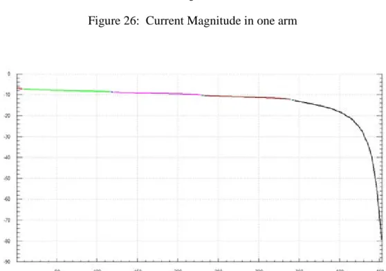
Figure 26 plots the current magnitude through the segments of one arm from bottom to top of the antenna. Figure 27 plots the corresponding current phase. The current

magnitude is symmetrical for the three arms at the first resonance as shown in Figure 25.

Figure 27: Current Phase in one arm Figure 26: Current Magnitude in one arm

Segment A mp s Segment D eg rees 44

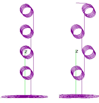
Additional analysis was performed on the orientation of the horizontal helical elements in each arm. The initial design depicted in Figure 21 was modified so that the direction of the coil turns in each helical element were opposite of the previous element. A single arm is depicted in Figure 28 for clarity; the analysis was performed with the three-arm

HMLA. Table 6 provides a comparison of the two configurations and shows the similarity in performance.

Table 6. Performance for three-arm HMLA, direction of helical coils modified

HMLA Mode ka Qz(ω) Resistance (Ω) Efficiency (%) r’/h original SHORT 0.33 107 24.74 86.2 1.20 modified SHORT 0.32 112 23.68 85.8 1.22 original OPEN 0.19 402 1.55 13.4 2.02 modified OPEN 0.19 403 1.54 13.2 2.06

Figure 28: HMLA single arm, original (left), modified with alternating turns (right)

2) Toroidal Helical Antenna and Variations

The new method can also be applied to canonical antenna designs such as the helical antenna. The helical geometry can be modified by replacing the straight wire sections with helical elements creating a toroidal helical antenna. An example of this geometry is presented in Figure 29. This design also provides additional options for inserting

toploading elements inside the volume for achieving lower self-resonant frequencies without increasing the overall volume of the antenna, and provides additional options for increasing wire length by modifying the radius and/or pitch of the helical coils. Figure 30 depicts the impedance and Figure 31 depicts the gain for a one-turn toroidal helical antenna as simulated using NEC.

Figure 29: One-turn toroidal helical antenna

Figure 30: Impedance for one-turn toroidal helical antenna

Figure 31: Gain for one-turn toroidal helical antenna

The self-resonant frequency of this design was further reduced by adding toploading in the form of a two-turn toroidal helical element on the interior of the antenna volume as depicted in Figure 32. These designs also allow for the use of folded arms to increase the antenna impedance in order to offset the reduction in resistance due to the increase in resonant wavelength. Figure 33 depicts the impedance and Figure 34 depicts the gain pattern for a one-turn toroidal helical antenna with inner toploading as simulated in NEC.

Figure 32: One-turn toroidal helical antenna with two-turn inner toploading

Figure 33: Impedance for one-turn toroidal helical antenna with inner toploading

Figure 34: Gain for one-turn toroidal helical antenna with inner toploading 49

A variation on the design theme is depicted in Figure 35 with four arms of one-half turn each and toploaded with a single circular wire. The base of each arm is short-circuited to the PEC ground plane to provide for symmetric current distribution. The circular wire provides for toploading without increasing the enclosed volume of the antenna. The combination of toploading for improving current distribution and folding for increasing input impedance result in optimized Q for a given ka. Figure 36 depicts the impedance and Figure 37 depicts the gain pattern for a four-arm toroidal helical antenna as simulated in NEC.

Figure 35: Toroidal helical antenna with four half-turn folded arms

Figure 36: Impedance for half-turn toroidal helical antenna, four folded arms

Figure 37: Gain for half-turn toroidal helical antenna, four folded arms 51

A comparison of toroidal antenna designs is listed in Table 7 where it is observed that folded arms (Figure 35) satisfied design requirements in terms of input resistance and Q.

Table 7. Helical MLA and Toroidal Helical Performance

Antenna Frequency (MHz) Resistance (Ω) ka Q Wire Length (meters) Helical MLA

(folded arm) Figure 21 15.6 20 0.36 111 34.1

Toroidal Helical

Figure 29 15.0 2.5 0.32 160 8.5

Toroidal Helical

(toploaded) Figure 32 8.5 2 0.19 355 48.0

Toroidal Helical

(folded arm) Figure 35 14.4 24 0.32 82 32.9

3) Observations

After analyzing numerous helical meandering line and toroidal helical designs, it was observed that both approaches provided for significant decreases in ka for HF band antennas. The concept of inner toploading was also demonstrated and experimentally verified using both design approaches. Resonant frequency, ka, and Q were all reduced by as much as 50% depending on the design approach selected, providing options when requirements or other size limitations restrict the allowable height or volume of the antenna.

E.

Investigation of Fractal Geometries

The term “fractal” has almost as many definitions as it does applications across various fields of study. One popular definition, published by Benoit Mandelbrot, is "a rough or fragmented geometric shape that can be split into parts, each of which is (at least

approximately) a reduced-size copy of the whole" [27]. In simpler terms, “fractal” can be used to describe patterns with a similar or repeating nature. The concept of self-similar nature is also applicable when using the terminology “fractal antenna” which is defined in the IEEE standard as “A multiband antenna having a self-similar shape at several different scales” [28]. A fractal antenna is usually designed through successive iterations of applying a generator function to a basis (or “initiator”) shape.

One practical use for fractal geometries is they provide a method for generating complex structures within a bounded region. This property, originally investigated by mathematicians such as Hilbert [29], has been applied successfully to the design of many types of antennas.

A particularly interesting parameter for analyzing fractals is the “fractal dimension”, advocated by Mandelbrot [27] and defined as the dimension D = log N / log(1/r) representing a bent line with N equal sides of length r. Calculation of the fractal

dimension for a Koch fractal structure is straightforward. The Koch geometry depicted in Figure 38 is observed to have four equal sections (N = 4) with lengths equal to one-third of the total length (r = 1/3). Using these values the fractal dimension is calculated to be D = 1.26186, in contrast to the Euclidean spatial dimensions of lines (1 dimension), planes (2 dimensions), and volumes (3 dimensions). This is relevant because one definition for

the term fractal requires that the fractal dimension “strictly exceed” the topological dimension in Euclidean space [27].

The image shown in Figure 38 can be used to generate a Koch monopole antenna design by replacing each unbroken line segment with the generator. The Koch fractal pattern emer