Spinal-Like Regulator Facilitates Control of a Two-Degree-of-Freedom Wrist

Behavioral/Systems/Cognitive

Spinal-Like Regulator Facilitates Control of a

Two-Degree-of-Freedom Wrist

Giby Raphael, George A. Tsianos, and Gerald E. Loeb

Department of Biomedical Engineering, University of Southern California, Los Angeles, California 90089

The performance of motor tasks requires the coordinated control and continuous adjustment of myriad individual muscles. The basic commands for the successful performance of a sensorimotor task originate in “higher” centers such as the motor cortex, but the actual muscle activation and resulting torques and motion are considerably shaped by the integrative function of the spinal interneurons. The relative contributions of brain and spinal cord are less clear for reaching movements than for automatic tasks such as locomotion. We have modeled a two-axis, four-muscle wrist joint with realistic musculoskeletal mechanics and proprioceptors and a network of regula-tory circuitry based on the classical types of spinal interneurons (propriospinal, monosynaptic Ia-excitaregula-tory, reciprocal Ia-inhibiregula-tory, Renshaw inhibitory, and Ib-inhibitory pathways) and their supraspinal control (via biasing activity, presynaptic inhibition, and fusimo-tor gain). The modeled system has a very large number of control inputs, not unlike the real spinal cord that the brain must learn to control to produce desired behaviors. It was surprisingly easy to program this model to emulate actual performance in four very different but well described behaviors: (1) stabilizing responses to force perturbations; (2) rapid movement to position target; (3) isometric force to a target level; and (4) adaptation to viscous curl force fields. Our general hypothesis is that, despite its complexity, such regulatory circuitry substantially simplifies the tasks of learning and producing complex movements.

Introduction

Extensive research of the past century led to the modern view of the spinal cord as a center for sensorimotor coordination rather than just a relay from brain to muscles. For example, locomotion can be produced and controlled entirely by the spinal cord and the peripheral sensorimotor apparatus by means of a central pat-tern generator and associated circuitry responsible for reflexive adjustments to various conditions, such as loads, obstacles, and perturbations (McCrea and Rybak, 2008). Various descending pathways from the cerebral cortex, cerebellum, vestibular appa-ratus, brainstem, etc., modulate the function of the intrinsic spi-nal circuitry rather than controlling directly the highly phasic activity of the individual muscles responsible for the movement (Lavoie et al., 1995; Ivashko et al., 2003).

By contrast, studies of arm and hand movements in primates have focused largely on correlating the activity of populations of neurons in motor cortex with measureable features of the concomitant motor behavior. Inferring causation, however, requires an understanding of the intervening neural circuitry and musculoskeletal mechanics (Loeb et al., 1996). Various stud-ies have shown that the indirect pathway via subcortical or spinal interneuronal systems contribute the majority of inputs to fore-limb motoneurons (Gelfan, 1964; Alstermark and Sasaki, 1985;

Kitazawa et al., 1993). These spinal interneurons receive inputs from the pyramidal tract (Isa et al., 2007) and also convergent input from many modalities and sources of primary somatosen-sory afferents (as well as extrapyramidal descending activity), and they exert divergent excitatory and inhibitory influences on many motoneuron pools (McCrea, 1986; Fetz et al., 1989). Direct cor-ticomotoneuronal projections are largely absent in opossums, rodents, cats, and lower primates (Rathelot and Strick, 2009), which are capable of fairly sophisticated, voluntary limb move-ments for prey catching and/or food handling.

Over the past 20 years, there have been several attempts to model the lower sensorimotor system for voluntary movement, but they were usually restricted to a hinge joint operated by an antagonist muscle pair and they usually incorporated only a small subset of the known spinal circuitry (Feldman, 1966; Bullock and Grossberg, 1992; Bullock et al., 1993; Bashor, 1998; Feldman et al., 1998; van Heijst et al., 1998; Ostry and Feldman, 2003; Lan et al., 2005; Maier et al., 2005). Loeb et al. (1990) introduced linear quadratic regulator design to find optimal solutions for reflex gains in a multisegment limb model (He et al., 1991), but there was no way to reconcile these gains with the actual inter-neuronal elements of the spinal cord.

The model of spinal circuitry presented here appears to be the first to consider the shifting patterns of muscle coordination needed to operate multi-muscle, multi-degree-of-freedom link-ages in a variety of complex sensorimotor behaviors described in the experimental literature. The model is called a spinal-like reg-ulator (SLR) because it embodies the multi-input, multi-output connectivity, and gain features of an engineering regulator (Loeb et al., 1990; He et al., 1991). The most salient emergent property of the whole system is that despite the complexity of the available Received Nov. 7, 2009; revised May 19, 2010; accepted May 25, 2010.

This work was supported by the National Science Foundation Engineering Research Center for Biomimetic Mi-croElectronic Systems. G.A.T. was supported by a Myronis Foundation Fellowship. We thank R. Davoodi, M. Kurse, J. Weisz, and D. Song for their technical assistance and insights and C. Ghez and E. Fetz for valuable discussions.

Correspondence should be addressed to Gerald E. Loeb, University of Southern California, Denney Research Building B6, MC1111, 1042 Downey Way, Los Angeles, CA 90089. E-mail: [email protected].

DOI:10.1523/JNEUROSCI.5537-09.2010

circuitry, many different combinations of command signals result in generally stable and desirable output behaviors.

Materials and Methods

The biomechanical model (Fig. 1) was imple-mented in MATLAB. The human hand was modeled as a cone with realistic mass and mo-ment of inertia. The cone was connected to a stationary forearm model via a joint with two degrees of freedom. The five muscles that op-erate the wrist (extensor carpi radialis brevis, extensor carpi radialis longus, extensor carpi ulnaris, flexor carpi radialis, and flexor carpi ulnaris) were approximated as four identical muscle models [Virtual Muscle (Cheng et al., 2000)] with parameters derived from morpho-metric and physiological data. The muscles were attached to the same point on the station-ary forearm but were attached symmetrically, 90° apart from each other to the base of the cone at their distal ends. The initial posture of the model was such that the apex of the cone pointed downward to the ground with the sta-tionary forearm aligned with the vertical axis as shown in Figure 1. The muscles actuated the cone about thex- andz-axes analogous to ex-tension–flexion and radial– ulnar deviation ro-tations of the hand, respectively. The roro-tations of the cone were limited to 75° using a vis-coelastic stop. The variation in moment arm during the range of all movements was tuned to be within a reasonable approximation to the parameters observed in a realistic human hand. Previously developed mathematical models of

muscle spindles (Mileusnic et al., 2006) and Golgi tendon organs (Crago et al., 1982; Mileusnic and Loeb, 2009) were used for proprioceptive feedback. We used only the primary output (Ia) of the spindles in our simulations, which provides both position and velocity feedback de-pending on separately modulated static and dynamic fusimotor con-trol. The spindle secondary afferents provide essentially pure muscle length information, but relatively little is known of their interneuro-nal circuitry in the spiinterneuro-nal cord. The output of the closed loop simu-lations was visualized in MusculoSkeletal Modeling Software (Davoodi et al., 2003).

Unlike the simple elbow joint that is used in many studies, the wrist joint presents additional challenges to the control system. The extra de-gree of freedom obviously adds to the mechanical complexity, but even more distinctively, the muscles controlling the wrist movement must switch their functional relationships based on the type of task performed. For example, during wrist extension the extensor muscles function as agonists and the flexor muscles function as antagonists, but during radi-al/ulnar deviation, the extensor muscles (as well as the flexor muscles) oppose each other. The spinal cord circuitry is intimately related to these functional relationships between muscles, so these dynamic relationships required a new classification and corresponding synapses/connections in our spinal cord model. In our terminology, we decided to call the adja-cent muscles “partial synergists” because they switch from agonist to antagonist based on the type of task. The diagonal muscles that were farthest apart from each other and that always opposed each other (for example, extensor carpi radialis and flexor carpi ulnaris) are designated as “true antagonists” and include only the classical reciprocal antagonist circuitry between them (Fig. 2). We modeled both synergistic and antag-onistic circuits between the partial synergists (Fig. 3) and let the control algorithm adjust the gains of each independently, thereby establishing functional synergist and antagonist relationships as required for each task.

The complete SLR model has 184 control inputs. We differentiated the inputs as “SET” and “GO” (Fig. 1), according to the terminology of Eliasmith and Anderson (2003). The “SET” inputs regulated the background activity in the spinal cord throughout the simulation and consisted of the gains of neural pathways, presynaptic inhibition, the subthreshold biases of the interneurons, and the fusimotor drive (␥ static and␥dynamic) to muscle spindles. The “GO” inputs initiated movement or other state changes and maintained the new state until the end of the modeled behavior. To explore the intrinsic properties of the spinal cord model and to test our hypothesis, we used the simplest descending inputs, namely step functions, as “GO” inputs. All simulations had a duration of 3 s and the background activity in the spinal cord was responsible for maintaining a steady posture of the hand for a specified initial time (1 s) before the impending “GO” input. The SET gains alone mediated the rapid reflexive response of the hand during perturbation in the passive postural stabilization task.

Spinal circuitry model

Modeling the neuron is often a tradeoff between biological realism and computational feasibility, especially when large numbers of neurons are involved, such as in the spinal cord model. The computational complex-ity of the model is one of the most critical factors in our simulations because hundreds of runs must be performed while the optimization algorithm converges to a desired solution. We modeled the input– out-put behavior of individual pools of interneurons and motoneurons using a sigmoidal transfer function (Eq. 1):

1

1⫹e⫺a共x⫺b兲, (1)

wherexis the input to the neuron, andaandbcontrol the slope and range of the sigmoid. The control inputs to interneurons were further

Figure 1. Biomechanical model. The human hand was approximated as a cone with realistic parameters (table). It was attached to a stationary forearm via a two-degree-of-freedom joint. Four realistic muscle models [Virtual Muscle (Cheng et al., 2000)] actuated the cone to produce force or motion in the extension–flexion direction (in plane of drawing) and radial– ulnar direction (perpendicular to plane of drawing). Proprioceptive sensors attached to each muscle provided proprioceptive feedback to the SLR. The SLR integrated proprioceptive feedback and descending commands to provide motoneuronal excitation to the muscles. These projections were associated with 184 control inputs that were differentiated as SET and GO inputs (see also Fig. 2). The SET inputs continuously regulated the background activity in the spinal cord and the GO inputs produced the transition to a new state.

differentiated as follows: (1) bias input that controlled the background activity in the interneuron (SET) and (2) supraspinal descending input that initiated movement (GO). The dynamic range of all neural activity was normalized between 0 and 1 and all inputs were constrained to the range⫾1. The nonlinearity in the sigmoidal model enabled the “reflex gating” described when biological systems switch between behavioral states. Throughout this article, we refer to “gains” as the input settings of these nonlinear operators in the regulator.

We extracted the structure and properties of the known pathways in the spinal cord from the literature (summarized by Pierrot-Deseilligny and Burke, 2005) and modeled five classical types of interneurons and the connectivity that they establish between the afferents from a given muscle and the motoneurons of the same (homonymous), synergist (heterony-mous), and antagonist motoneuron pools (␣in Figs. 2, 3).

Propriospinal pathway.The proprioceptive sensory outputs (muscle spindle primary Ia and Golgi tendon organs Ib) excited the propriospinal pathways (PN in Figs. 2, 3) (Malmgren and Pierrot-Deseilligny, 1988a; Gracies et al., 1991; Burke et al., 1992). The propriospinal circuit models directly excited the homonymous motoneurons and also formed the following connections with other motoneurons: “selective” synapses whose gain could be excitatory or inhibitory for the partial synergists and inhibitory synapses for the true-antagonist muscles.

Monosynaptic Ia excitation pathway.Muscle spindle primary afferents excited the motoneurons monosynaptically (Malmgren and Pierrot-Deseilligny, 1988a). The afferents also excited the heteronymous mo-toneurons of partial-synergist muscles (Lloyd, 1946; Meunier et al., 1993).

Reciprocal Ia inhibition pathway. The Ia-inhibitory interneuron re-ceived monosynaptic input from Ia afferents and provided inhibitory projections to true-antagonist and partial-synergist motoneurons (Tanaka, 1974; Pierrot-Deseilligny et al., 1981; Crone et al., 1987), as well

as disynaptic recurrent inhibition (disinhibi-tion of antagonists via the Renshaw pathway) from homonymous motoneurons (Hultborn et al., 1971). The Ia interneurons were themselves inhibited by the corresponding true-antagonist and partial-synergist Ia interneurons (Hultborn et al., 1976).

Renshaw inhibition pathway.Renshaw inter-neurons (R in Figs. 2, 3) formed recurrent con-nections with homonymous motoneurons. They were also excited by motoneurons of partial-synergist muscles (Eccles et al., 1954, 1961). They inhibited both partial-synergist motoneurons and true-antagonist Renshaw interneurons (Hultborn et al., 1979; Ryall, 1981).

Ib-inhibitory pathway.The Ib interneuron re-ceived excitatory input from Golgi tendon organs. The dominant effects of the Ib interneu-ronal circuitry were inhibition of homonymous motoneurons, excitation of true-antagonist mo-toneurons, and either excitation or inhibition of partial-synergist motoneurons (Eccles et al., 1957).

Excluded spinal circuitry. We excluded other known interneurons and connections listed below to limit the complexity of the model and to minimize the number of arbitrary decisions required to model poorly characterized path-ways. The most detailed studies of wrist sensori-motor circuitry are in the cat, but comparisons with monkeys and humans suggest substantial refinements related to the substantially changed mechanics and behavioral repertoire of limbs used for manipulation rather than locomotion (for review, see Illert and Ku¨mmel, 1999). Be-cause the SLR model proved to be surprisingly tractable computationally, it would be feasible to add other circuits in the future, but this would be useful only to account for behaviors that the model cannot perform well. As described below, the SLR as modeled accounted well for all motor tasks attempted so far.

All cutaneous input was omitted because the tasks to be modeled can be performed without it and because the details of these oligosynaptic circuits (e.g., Hongo et al., 1989a,b) are poorly described in man.

The excitatory and inhibitory group II interneurons as well as all group II projections from the muscle spindles were omitted because their con-nectivity is not well characterized (Lundberg et al., 1987; Jankowska, 1992). Furthermore, the excitatory and inhibitory group II pathways parallel the Ia pathways to a great extent, suggesting a functional similar-ity between them (Lundberg et al., 1987). The variable␥-static and

␥-dynamic gains in our model allow for the adjustment of the relative sensitivity of Ia fiber activity to muscle length and velocity, so it captures to some extent the group II contribution to movement.

The known but poorly defined pattern of Ia projections to Ib interneu-rons (Jankowska, 1992) was omitted. An important property of this con-vergence is that it provides a reflexive adjustment of the firing sensitivity of the Ib interneuron with respect to the phase of the movement. This may be especially important for simulating more complicated tasks, and we plan to incorporate some of these projections in future models.

The disynaptic inhibition of propriospinal interneurons (Illert et al., 1975) was omitted. The apparently diffuse connectivity of these cutane-ous and proprioceptive inhibitory effects (Alstermark et al., 1984) sug-gests that they may be responsible for setting the bias of the propriospinal interneurons (SET input in our model), while the more specific excita-tory projections (Illert et al., 1978; Malmgren and Pierrot-Deseilligny, 1988b) seem more likely to mediate functional relationships among the muscles and their modulation during the dynamic phase of the move-ment. Furthermore, the feedback inhibitory interneurons are more

Figure 2. Spinal circuitry between true antagonists. The diagonal muscles are called true antagonists because they oppose each other in all tasks. There are two such circuits in the integrated model. Five interneuronal pathways were modeled: (1) PN— propriospinal, (2) monosynaptic Ia-excitatory, (3) reciprocal Ia-inhibitory, (4) R—Renshaw inhibitory, and (5) Ib-inhibitory pathways. The inputs are differentiated as SET and GO. The SET inputs regulate the background activity in the spinal cord and consist of the gains in the neural pathways plus Ia presynaptic inhibition (small white circles marked S in the figure), and biases to the interneurons and motoneurons and fusimotor drive (␥static and␥dynamic) to the muscle spindles (the large white circles marked SET).

sensitive to input from cutaneous fibers (Malmgren and Pierrot-Deseilligny, 1988b; Alstermark et al., 2007), which could be es-pecially important for tasks that include state transitions, such as between reach and grasp, which we have not modeled.

Commissural interneurons were excluded from our model principally because the details of their connectivity are largely unknown and they appear not to be especially important for the tasks that we are simulating. Their bilateral projections in the spinal cord, mostly to other segmental interneurons, suggest that they may be primarily responsible for coordinating mo-tion of contralateral limbs, such as in locomo-tion (Jankowska, 2008).

All the supraspinal descending inputs pro-jected only to the interneurons; the␣ motoneu-rons received no direct descending commands, but the integrative outputs of the interneurons converged at the␣motoneurons (Figs. 2, 3). This is a key distinction compared to previous models of spinal circuitry (Feldman, 1966; Bul-lock and Grossberg, 1992; BulBul-lock et al., 1993; Bashor, 1998; van Heijst et al., 1998; Ostry and Feldman, 2003; Lan et al., 2005; Maier et al., 2005), but it is more consistent with the actual neuroanatomy. This also appears to be the first model of spinal cord circuitry to deal with the shifting patterns of synergistic and antagonistic muscle activity that necessarily accompany multimuscle, multi-degree-of-freedom systems.

Optimized control of the spinal cord model

We simulated four behavioral tasks for which human performance data were available for comparison (literature references and rationales are provided with the Results): (1) brief perturbing torque pulses (100 N⫻ 10 ms) in various directions to the hand in the initial, neutral posture; (2) rapid voluntary movement to a target posture (35° wrist extension) with a perturbing torque pulse; (3) rapid development of isometric force to a target level (either 60 N extension as a sustained step or 70 N extension as a transient pulse); and (4) adaptation to viscous curl field (rapid volun-tary wrist extension performed in the presence of perturbing radial torque proportional to instantaneous velocity in extension).

We anticipated that it would be difficult to use random optimization to solve such a complex, high-dimensional system, so initially we tried setting various gains “by hand” according to our intuition as neurophysi-ologists and control engineers. We found that it was surprisingly easy to reproduce each of the experimental behaviors by adjusting a small subset of descending controls (see examples in Fig. 4 described below). Further-more, emergent details of stability and muscle recruitment were quite realistic, even though we made little or no attempt to optimize the values of the many other control signals and we did not modulate any of the control signals. In fact, these behaviors appear to be robust emergent properties of the complete set of spinal circuitry as modeled. We then optimized all 184 control inputs (gains) using a custom gradient descent algorithm based on a simple quadratic cost function (Eq. 2) that penal-ized any deviation from the desired trajectory or state:

cost⫽

冕

The steps in the gradient descent algorithm are as follows: (1) Random values were assigned to the control inputs initially (Monte Carlo method). However, we avoided extreme values (less than ⫺0.5 and greater than 0.5) to prevent instability in the system. (2) A single control input was picked at random from the pool and optimized individually. (3) Two simulations were required to optimize each control input. The

first simulation perturbed the starting control input in the positive direc-tion and the second perturbed it in the negative direcdirec-tion. The value of the control input that produced the lowest cost was retained. (4). We used an “annealing curve” strategy when perturbing the control inputs, by starting with a higher value initially (⌬ ⫽ ⫾0.2) and then reducing it for later iterations (usually by successive factors of 2 but see Discussion). (5) One iteration of the model was said to be completed when all control inputs in the model had been optimized once. (6) The whole model was then iterated multiple times until the overall cost converged to a low value.

A cocontraction index was computed for all the tasks using Equation 3, in which cocontraction is quantified as the product of the activation levels in the two pairs of true-antagonist muscles:

Cocontraction index⫽

冕

This was used only to compare converged solutions, not as a component of the cost function used during optimization.

Results

Stabilizing response to external force perturbation

The nervous system has multiple mechanisms to counter external perturbations to the limb. The impedance of the musculoskeletal system itself created by inertial properties of the limb (force-acceleration) plus spring-like (force-length) and viscous-like (force-velocity) properties of the active muscles produces zero-delay resistive forces against sudden perturbations called “pre-flexes” (Loeb et al., 1999; Brown and Loeb, 2000). High levels of muscle coactivation are energetically inefficient and likely to in-terfere with rapid movement, so short-latency “reflexes” gener-ated by proprioceptive sensors and transmitted through the Figure 3. Spinal circuitry between partial synergists. The adjacent muscles are called partial synergists because they switch form synergists to antagonists based on the task performed. There are four such circuits in the integrated model, each consisting of five interneuronal pathways and their SET and GO controls (same abbreviations as Fig. 2).

circuits in the spinal cord also play a major role in resisting expected perturbations. Both “preflexes” and “reflexes” are un-der the control of the nervous system, which can effectively preprogram them to deal with expected perturbations. The “pre-flexes” depend on the activation level of the muscles and “re-flexes” are largely governed by the background activity in the spinal cord and the levels of ␥-static (bias control) and ␥-dynamic (viscosity control) inputs to the muscle spindles.

We applied an external force pulse of magnitude 100 N and duration 10 ms along the direction of wrist flexion to the isolated biomechanical model detached from the spinal circuitry. The passive model displayed damped oscillations about the wrist joint typical of a spring-mass-damper system (Fig. 4a, dashed line). The time period of oscillation increased when gravity was re-moved from the system, indicating that gravity was a weak stabi-lizing force.

The magnitude and efficacy of preflexes depends greatly on the level of background activation (sometimes referred to as “stiffness” or “tone”) in the musculoskeletal system. We applied the same external force perturbation after attaching the spinal circuitry and feedback sensors to the plant. The hand stabilized back to the resting position in about 600 ms (Fig. 4a, solid line), demonstrating the stabilizing property of the spinal cord. The gains in the spinal cord were mostly left at a low value and re-quired only minimal intuitive adjustment to produce a physio-logical response based on reciprocal muscle activation (Fig. 4b,c). The model continued to provide a good response even after the removal of gravity from the system.

When the gradient descent algorithm was used to adjust the background activity in the spinal cord (by optimizing the SET commands), it converged rapidly and stabilized the hand in 200

ms (Fig. 4d). Importantly, the solutions produced by our model did not rely exces-sively on cocontraction (see Fig. 9cbelow), but rather agreed well with experiments in which the opposing wrist muscles were anesthetized to prevent any cocontraction (Hore et al., 1990).

Rapid voluntary movement to a position target

Corticospinal trajectory generation for vol-untary reaching movements is assumed to shift from control of slow movements via visual and proprioceptive feedback to con-trol of rapid movements via a feedforward trajectory generator with superimposed dynamic error compensation (Cisek et al., 1998). To identify the potential contribu-tion of the spinal cord to fast movements, we simulated a rapid, stable wrist exten-sion from neutral to 35° in our model (Fig. 4e). The behavior was further tested for stability by applying a brief torque pertur-bation (100 N, 10 ms) during the hold phase of the movement (at 2.3 s simulation time). It was easy to obtain physiologically realistic performance by adjusting indi-vidually the feedback gains (SET) and simple step inputs (GO) to the proprio-spinal interneurons (Fig. 4e). When the complete set of gains was optimized using the gradient descent algorithm, perfor-mance converged rapidly and tracked the desired trajectory (dot-ted line) even more closely (Fig. 4g). The optimized solution also displayed a faster response to perturbation (Fig. 4g).

Voluntary isometric force to a target level

While the first burst in the agonist muscle is present under both isometric and anisometric conditions, the second burst in the antagonist and the third again in the agonist (so-called triphasic burst pattern) were reported to be missing under isometric con-ditions in early experiments on cats (Ghez and Martin, 1982). A few years later, the same laboratory (Ghez and Gordon, 1987) studied the role of opposing muscles in the production of isomet-ric force trajectories in human subjects and found that for brief force rise times (⬍120 ms), reciprocal activation of the antago-nist muscle occurred consistently. In the experiment, the subjects had their arm immobilized, and they were asked to produce force to a specified target level. The authors interpreted this muscle activity as indicative of similar preprogrammed phasic drive from the motor cortex. We replicated the experiment in our model by constraining the wrist joint using a viscoelastic restrictor with that permitted 2 mm of motion at peak force, similar to what seemed likely to be present between the bones and the apparatus through skin and padding. This results in small but potentially important departures from the purely isometric assumptions un-derlying this interpretation.

Gradient descent was used to optimize the SET and GO inputs to the force trajectory for rapid force steps (Fig. 5a) and force pulses (Fig. 5b). Rapid modulation of agonist activity (Fig. 5c,d) could be explained by modulation of spindle afferent activity (not illustrated) as a result of stretch of their elastic tendons. Antago-nist bursts were produced for rapid force modulations (Fig. 5c) Figure 4. a– d, Stabilizing response to external force perturbation.a, Rotation of the hand from rest position (dotted black line)

about flexion– extension direction in response to a force pulse perturbation in the flexion direction (magnitude 100 N, duration 10 ms) at 1 s simulation time. The passive musculoskeletal model alone produced damped oscillations in response to the perturbation (dashed line). With the hand-tuned SLR model attached, the hand stabilized back to the resting position in 600 ms (solid line).b, Output from the extensor (red) and flexor (blue, plotted downward) motoneurons.c, Corresponding extensor (red) and flexor (blue) muscle force modulation.d, Response to perturbation after optimizing the control inputs (SET inputs) using gradient descent algorithm (solid black line).e– h, The hand stabilized back to the resting position in 200 ms. Rapid voluntary movement to a position target.e, Rotation of the hand to 35° extension and response to the same force pulse perturbation in the extended position with minimal intuitive adjustments of the gains and step inputs to the propriospinal interneurons.f, Corresponding extensor (red) and flexor (blue) muscle force modulation.g, Trajectory (solid black line) after optimizing the control inputs (SET and GO) to the desired trajectory (dotted black line) using gradient descent algorithm.h, Corresponding extensor (red) and flexor (blue) motoneuron outputs.

but were absent for slower force trajectories (Fig. 5d), as was reported experimentally (Ghez and Gordon, 1987). These were associated with the smaller modulations of their homonymous spindle afferents as a result of the compliance of the viscoelastic restrictor.

Adaptation to viscous curl force fields

The adaptation of human reaching to novel dynamic environ-ments, such as an opposing curl field, has been widely accepted as one of the most valuable testbeds for the notion of internal mod-els and the learning process involved in their development and adaptation [see Kluzik et al. (2008) for recent examples of this extensive literature]. In the experiment, the subject makes reach-ing movements with a robot that generates a perturbreach-ing force proportional to the velocity of the actual movement and perpen-dicular to the direction of intended movement. The trajectories are initially skewed in the direction of the perturbation but grad-ually straighten with adaptation. When the field is unexpectedly removed, the trajectories show mirror-image aftereffects.

In an attempt to find the limits of the spinal cord’s potential role in motor adaptation, we replicated the experiment in our model. We defined the intended direction of movement of the hand about thex-axis (flexion– extension) and applied viscous perturbing force about thez-axis (radial– ulnar deviation) in pro-portion to the velocity in thex-axis. Figure 6 illustrates the sur-prisingly good performance obtained using a simple gradient descent solution with unmodulated SET and GO descending

commands for gains. The extension movement (Fig. 6a) follows the desired trajectory almost as well as for the unopposed exten-sion solution in Figure 4g; the initial radio-ulnar deviation of about 35° before training has been reduced to almost zero (Fig. 6b). The mechanisms that underlie this performance appear to involve a combination of asymmetrical fusimotor gains (Fig. 6e) and asymmetrical activation of propriospinal neurons (Fig. 6g) Figure 5. Voluntary isometric force to a target level.a, The net reaction force (solid black

line) produced by the isometric muscles after optimizing the control inputs to the desired force (dashed black line) using gradient descent algorithm.b, Pulse force trajectory (solid black line) produced after optimizing the control inputs using gradient descent algorithm.c, Agonist (red) and antagonist (blue) motoneuron output for brief rise time (100 ms) pulse-force trajectory. Tasks replicating brief rise time force trajectories (⬍120 ms) consistently produced antagonis-tic pulses in both pulse and step force trajectory tasks.d, Agonist (red) and antagonist (blue) motoneuron output for long rise time (250 ms) step-force trajectory task. The antagonist pulse was distinctively absent for intermediate (120 –200 ms) and long (⬎200 ms) rise time force trajectory tasks.

Figure 6. Adaptation to viscous curl force fields.a, Tracking a desired trajectory (dotted black line) in the presence of viscous force field perturbations. The gradient descent algorithm optimized the control inputs to produce extension (solid black line) that closely tracked the desired trajectory.b, Radio-ulnar deviation in the presence of viscous curl force fields reduced from 35° to nearly 0° (solid black line) after optimization.c,d, After-effects when the curl force field was removed.e, Primary afferent response from the muscle spindles in each of the four muscles after adaptation (two extensor muscles in red plotted upward; 2 flexor muscles in blue plotted downward).f, Responses from the four Golgi tendon organs after adaptation.g, Output of motoneurons exciting the extensor muscles (red) and flexor muscles (blue), after adaptation.h, Extensor (red) and flexor (blue) muscle force modulation after adaptation.

and resulting muscle force (Fig. 6h). The aftereffects are also surprisingly physiological when the curl field is removed from a system that has adapted to it (Fig. 6c,d).

To explore the variability of adaptation across subjects, we took advantage of the fact that the SLR generally produces many “good enough” solutions for any given task when started with random initialization gains (see Fig. 7 below). We used several such solutions for unperturbed, rapid wrist extension as starting points for adapting to the curl fields. This resulted in generally adequate but substantially different performance for these func-tionally equivalent starting points, in terms of speed of conver-gence to a solution, quality of the solution, and the magnitude of aftereffects. This would be consistent with the general observa-tion that subjects differ in how quickly they learn to compensate for unusual and complex loads such as curl fields [e.g., Shadmehr and Mussa-Ivaldi (1994), their Fig. 11].

The subjects in force-field experiments showed aftereffects of force adaptation even though they had explicit knowledge that no external force would be applied to the reaching hand (Kluzik et al., 2008). This suggests that force adaptation cannot be switched on or off by cognitive cues alone but may also involve a spinal level adaptation that takes time to readjust. In the SLR, the errors produced due to the unexpected dynamic changes were trans-duced by the proprioceptive sensors, which in turn evoked re-flexes to reduce the error. Our results suggest that the gains in the regulator circuitry can be readjusted to eliminate these trajectory deviations almost completely. We acknowledge that the model does not account for various other observations in the experiments, such as the generalization of adaptation across arms that appears to be in the extrinsic coordinates of the task (Criscimagna-Hemminger et al., 2003). There are substantial interhemispheral connections as well as uncrossed descending circuits and bilateral commissural spinal in-terneurons (which we have not modeled) that may contribute to such generalization, even without an explicit internal model in ex-trinsic coordinates.

Multiple local minima

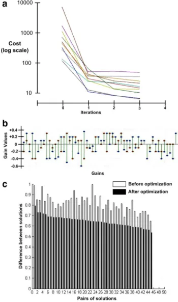
Figure 7ashows learning curves for 10 solutions of rapid ramp-hold movements, all initialized to different random settings. Cost reflects the deviation from the desired trajectory as defined in Equation 2. Even though the initial cost values were considerably different, all converged rapidly to stable solutions. The final val-ues were distinctly different from each other but were all within typical variability of experimental performance (note log scale of cost function). We further examined the solutions themselves to see how they differed from each other. Figure 7bcompares the final values (ordinate axis) for 54 of the gains from two of the solutions from Figure 7athat achieved very similar cost and ki-nematic details. They differ substantially in many details, often including both magnitude and sign. This suggests that the state space consists of many, widely separated local minima that can be used to perform the task successfully.

We further tested the distribution of local minima by exam-ining the distances between the starting and final positions in the high-dimensional state space of gains (square root of the sum of Figure 8. Typical learning curve for each task. All tasks started with random starting values for the control inputs, which were then optimized using gradient descent algorithm. One iter-ation of the model was said to be completed when all control inputs in the model had been optimized once. The common feature across all tasks was that almost all of the cost reduction was obtained in the first iteration with little improvement in subsequent iterations.

Figure 7. Analysis of gain values.a, Learning curves for 10 solutions of rapid ramp-hold movements all initialized to different random settings. Even though the initial cost values were considerably different, all curves converged rapidly to stable solutions.b, The final values (or-dinate axis) for 54 of the gains from each of two solutions (red and blue circles) fromathat achieved very similar cost and kinematic details. They differ substantially in many details, often including both magnitude and sign.c, Distance between the starting and final positions in the high-dimensional state space of gains (square root of the sum of squared distances in all 200 gain axes). The 45 possible pairwise comparisons, ordered according to their distances from each other after optimization.

squared distances in all 184 gain axes), il-lustrated in the bar graph in Figure 7cfor the 45 possible pairwise comparisons, or-dered according to their distances from each other after optimization. There was a weak tendency for solutions that were close to each other in space to have started closer to each other initially, consistent with the expected properties of gradient descent. There was no tendency for the normalized cost differences of the start-ing positions or optimized solutions to correlate with separation of the solu-tions in state space, consistent with the notion that the local minima are widely distributed throughout the state space and not greatly different in actual values or local steepness.

Learning rate

Across all the simulated tasks, we noticed a consistent and prominent characteristic in the gradient descent process, regardless of task complexity, random starting posi-tions, or initial performance: The vast majority of the reduction in cost was ob-tained in the first iteration, which used the biggest step change in gain. In all our sim-ulations, we used a fairly shallow “anneal-ing curve” strategy, start“anneal-ing with a larger change in gain in the first iteration (⌬ ⫽

⫾0.2) to escape from poor local minima and then reducing the change to smaller values (typically⫾0.1,⫾0.05,⫾0.01) in subsequent iterations. Figure 8 shows one illustrative solution for each of the five tasks that we have modeled. Further opti-mization from this point produced only very small reductions in the cost even though there were substantial changes in the gains, indicating broad local minima. We have tried several different annealing curves (patterns of decreasing gain steps explored in successive iterations), but this finding appears to be robust, suggesting that most local minima are well separated from nearby local minima. Clearly, under some circumstance it may be desirable to force systems out of local minima to find the global minimum for truly optimal performance, as opposed to “good enough” performance. That may require more complex gradient descent strategies in which more than one gain is varied at a time. This notion seems to have some

sub-jective resonance with the strategies used by coaches to force athletes out of “bad habits” (Lyndon, 1989).

Comparison with servo control

To compare the performance of our model with a sufficiently complex model with the same sensors and actuators but without the specific interneuronal types, we developed a classical servo-control model and replicated the same five tasks. The

motoneu-rons received direct feedforward commands plus homonymous positive and negative feedback from the muscle spindle and Golgi tendon organs, respectively (Fig. 9a), similar to the “autogenetic stiffness servoregulator” proposed by Houk (1979). The only non-homonymous projection to the motoneuron was the nega-tive feedback from the true-antagonist muscle spindle. The mean performance cost produced by the new model was significantly higher in all the tasks compared to the SLR model (Fig. 9b). Even Figure 9. Servo-control model.a, Circuit diagram of a classical servo-control model. The motoneurons received direct feedfor-ward commands plus homonymous positive feedback from the muscle spindle primary afferents and negative feedback from the Golgi tendon organs. They also received negative feedback from true-antagonist muscle spindle primary afferents. All of these commands and gains and fusimotor biases were adjusted by random gradient descent as for the SLR model.b, Cost comparison between the servo-control model, SLR model, and experimental performance (Liles, 1985; Ghez and Gordon, 1987; Wierzbicka et al., 1991) is shown for each of the tasks we modeled. The shaded box with the dotted outline represents performance levels for those subjects who adopted muscle coactivation rather than the more typical triphasic burst pattern.c, Cocontraction comparison similar tob; see text.

for relatively good performances, servo control produced un-physiological levels of cocontraction in muscles (note log scale in Fig. 9c), a strategy that is highly inefficient because it requires high metabolic energy. The optimized performance of the servo con-troller was highly sensitive to the starting values of the gains and some solutions had large deviations from the desired behavior. The local minima in the solution space appeared to be very broad and it was often difficult to escape from poor minima even with multiple iterations. In contrast, the SLR model produced perfor-mance costs that were always within observed experimental vari-ability regardless of initialization conditions, and the mean and SDs of the costs across similar tasks were considerably lower. The SLR model relied heavily on proprioceptive feedback to improve performance in all the tasks with little cocontraction (Fig. 9c). The local minima in the solution space were quite robust and in all cases were adequate to produce physiologically realistic performance.

Sensitivity of optimized solutions

The tendency of the learning curves to plateau rapidly at low costs regardless of annealing curve (Figs. 7, 8) suggests that the opti-mized solutions of the SLR model were relatively robust to changes in individual gains. A more systematic test of this was generated for a typical converged solution for the rapid voluntary extension task. After three iterations with⌬ ⫽0.1 for all gains, the cost had plateaued to the low level indicated at⌬ ⫽0 in the center of Figure 10a. From that starting gain set, each gain was system-atically varied by steps of⫾0.05,⫾0.1, or⫾0.2, resulting in a family of changes to the cost. The introduction of the finer steps of 0.05 resulted in small improvements for some gains, as ex-pected. Some of the gains had little effect on this task; those same gains were often more critical for other tasks (e.g., gains related to force feedback tended to be more important for the isometric force tasks). A few of the gains (thick lines with symbols; key in legend) had steeper effects on performance, often for changes in one direction but not the other. Because the starting values of these gains could vary from 0 to⫾1, the fractional value repre-sented by these⌬values varied widely and might be more rele-vant to their sensitivity to neural noise. The values for⌬ ⫽ ⫾0.05 were replotted as percentage change in Figure 10b, with infinity denoting starting gains of zero. Two of the gains were still quite sensitive in both directions, but their effects were reciprocal, so that an increase in one could be cancelled by a decrease in the other. Interestingly, the synergistic extensor muscle that must work symmetrically in this task did not exhibit a similar pattern of sensitivity. After deliberately fixing either of these most sensi-tive gains to a value that produced high cost, running one itera-tion to adjust the remaining gains was able to reduce the cost back down to the human performance range (dashed lines). This was accomplished by changing a large number of gains depending on the random order in which they were tested, not necessarily the gain exhibiting the reciprocal relationship noted above. These findings are consistent with the low costs after the initial itera-tions with the relatively coarse⌬ ⫽0.1 and the broadly different gain solutions with similar performance (e.g., Fig. 7b).

Generalization of optimized solutions

One important property of motor strategies learned under one set of conditions is that they generalize to other, similar condi-tions that were not part of the training set. We tested whether this was a property of the SLR strategies to resist brief force perturba-tions such as that illustrated in Figure 4d. Initially we trained the SLR to resist force perturbations in the four perpendicular

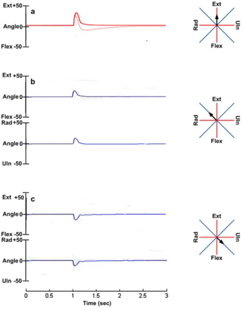
ana-tomical axes of the wrist, i.e., flexion, extension, radial, and ulnar directions (Fig. 11, red axis lines). The algorithm thus optimized the gains to reduce the sum of the costs calculated from pertur-bations in all four anatomical axes, delivered sequentially, one after the other. After training the converged solution set provided good response to perturbation in all four trained directions. We then tested the ability of the converged solution to resist similar perturbation in new untrained directions, such as pulling direc-tions of the individual muscles, i.e., rotated 45° from the anatom-ical axes (Fig. 11, blue axis lines). The responses were almost equally rapid and accurate as for the trained directions (Fig. 11). Thus one solution set was able to generalize and resist perturba-tion in any direcperturba-tion in the workspace.

Discussion

Limitations of the model

The selection and design of the modeled components entailed many omissions and simplifications from the known physiology and mechanics of this neuromusculoskeletal system. Despite these limitations, it was relatively easy for a simple gradient de-Figure 10. Sensitivity analysis.a, Starting with a set of converged gains after three itera-tions with⌬ ⫽0.1, each gain was individually adjusted up and down by⌬values of 0.05, 0.1, and 0.2 and the resulting cost plotted on the ordinate; dashed lines indicate range of normal human performance. Traces exhibiting high sensitivity in at least one⌬direction are high-lighted in color (key: red down arrow⫽GO drive to propriospinal interneuron to EU muscle; green up arrow⫽SET drive to same; mauve circle⫽GO drive to propriospinal interneuron to FR; purple square⫽SET drive to same; green star⫽Ib feedback to FU).b, Cost values for⌬⫽ ⫾0.05 replotted as percentage gain change on abscissa (“inf” denotes starting value⫽0).

scent learning algorithm to achieve realis-tic performance in terms of both the performance goals of the task and realistic patterns of muscle activation regardless of starting conditions. Nevertheless, it is worth asking whether these simplifications themselves contributed to this finding. They include the symmetrical arrange-ment of the muscles, the sigmoidal input– output functions for all the neurons [omitting more complex nonlinearities such as plateau potentials (Hultborn, 2002)], and the omission of certain classes of interneuronal connections as detailed in the Materials and Methods. The servo-control model shared these properties but was notably less successful. Thus, some sort of regulator-like structure may be necessary, at least when the command structure is assumed to be highly limited (e.g., SET and GO step functions as used herein). The modeled spinal-like regula-tor appears to be sufficient under such cir-cumstances, but it would be interesting to replace some modeled pathways with some excluded ones whose connectivity suggests similar functionality, and then to compare their performance. It is also pos-sible that inclusion of some of the omitted pathways will be required to control more difficult tasks or more complex musculo-skeletal systems. We are now extending the SLR to control a two-joint planar arm that includes both uniarticular and biar-ticular muscles (Tsianos et al., 2009), a well studied experimental preparation that presents a richer set of biomechanical challenges. In the future, we hope to re-place the SLR circuitry with equally com-plex sets of interneurons with randomized connections to understand whether the capabilities of the SLR arise from its spe-cific patterns of connectivity as described in the literature or are simply an emergent property at a critical level of complexity.

The general utility of regulators

The SLR has a large number of control points, but it turned out to be surprisingly easy to find simple patterns of descending inputs that caused it to replicate actual performance details of a wide range of motor behaviors. This appears to be a conse-quence of the state space defined by the SLR, which has many local, “good enough” minima for each of the tasks we simu-lated. Importantly, regardless of starting gains, the SLR never became trapped in a local minimum that produced less than satisfactory performance. Against common intuition, we found that the larger the number of inputs that were opti-mized by the algorithm, the faster it converged to better per-formance. This is in contrast to the servo-control model, which converged more slowly and often to poor solutions. Poor performance, but not slow convergence, might reflect the substantially fewer interneurons and adjustable gains in the servo controller compared to the SLR.

One obvious complexity that we have avoided concerns the temporal modulation of descending commands during tasks. We were surprised by the range of dynamic behaviors that the model could reproduce using simple SET and GO step functions, but we expect this to break down for more complex tasks. Recordings of cortical activity during even simple tasks often show substantial temporal modulation that is more complex than a step function centered on the task initiation (Churchland and Shenoy, 2007). In fact, these patterns seem to have more in common with the wide variety of patterns described for spinal interneurons (Maier et al., 1998; Perlmutter et al., 1998) than with the canonical pa-rameters describing the task kinematics (e.g., direction, distance, velocity) or kinetics (e.g., individual muscle activity). Interest-ingly, complex EMG patterns in monkey arm muscles were sur-prisingly well predicted from cortical single-unit activity using nonlinear combinatorial functions such as might be embodied in spinal interneurons (Song et al., 2008) rather than more simple combinations (Westwick et al., 2006).

Figure 11. Ability of SLR strategy to generalize to new task conditions.a, Response to brief force perturbation along the extension direction (black arrow) before (dotted red line) and after (solid red line) training the SLR to resist in the anatomical axes of the wrist, i.e., flexion, extension, radial, and ulnar directions (red axes lines).b, Rotation of the wrist along ext-flex and rad-uln axes in response to the same force perturbation along untrained axes (blue axes lines), the pulling direction of the ECR muscle.c, Response of the SLR due to perturbation along the pulling direction of FCU muscle.

It is also important to consider the effects of intertrial variabil-ity in the descending commands. Churchland et al. (2006) deter-mined that⬃50% of the variance in performance was already present in these cortical neural signals rather than arising from the “motor noise” that has been attributed to discrete recruit-ment of size-ordered motor units (Jones et al., 2002). It is also likely that the cortical variability is itself correlated among mul-tiple units (Maynard et al., 1999). Churchland et al. (2006) inter-preted this variability as noise, but it may be indicative of purposeful exploration of the complex solution space afforded by an SLR to which these neurons project. Such exploration might be useful to free up the limited computational capacity of cortex so that other tasks can be learned. Doyon and Benali (2005) at-tributed the later stages of motor consolidation to redistribution via the corticostriatal or cortical-cerebellar systems, but it may also depend on the solution space of the SLR. Adding noise or purposeful variability to the command signals that are responsi-ble for setting the SLR gains during iterative adjustment seems likely to prevent the solution from settling into local minima for which any individual gain has a steep cost function (see Fig. 10 and related Results regarding sensitivity).

Interpretation of deafferentation experiments

Many researchers attribute a dominant role to descending com-mands rather than segmental feedback because studies have shown that both chronically and acutely deafferented subjects can produce some temporal details of normal muscle activation, specifically a triphasic burst pattern during rapid movements that is similar to that produced by normal subjects (Hallett et al., 1975; Rothwell et al., 1982; Sanes and Jennings, 1984; Forget and Lamarre, 1987; Berardelli et al., 1996). These results, however, do not prove that the behavior is normally achieved via open loop commands. It is possible that in the absence of sensory feedback to the regulator, the brain could have learned to produce a similar motor program, given that it is a necessary strategy of muscle recruitment for performing the task successfully. Interestingly, a deafferented patient exhibited a triphasic burst pattern in a study by Forget and Lamarre (1987) but was unable to produce it two years prior. Furthermore, chronically deafferented patients ex-hibit significantly different EMG timing and worse kinematic performance (Rothwell et al., 1982; Forget and Lamarre, 1987; Gordon et al., 1987), which could mean that the brain is intrin-sically an inferior source of such rapidly modulated motor com-mands compared to a regulator with phasic afferent feedback.

The acutely deafferented patients in the study by Sanes and Jennings (1984) were able to produce remarkably crisp EMG patterns and relatively better kinematic performance than the chronically deafferented patients of the other studies. However, the ischemic block that they imposed affected afferent activity from muscles below the elbow, leaving intact both the efference copy from their motoneurons via the Renshaw interneurons and all proprioceptive feedback from all proximal muscles. The wide-spread extent of such feedback circuitry (Cavallari et al., 1992) and the strong modulation of proximal muscles to stabilize pos-ture during phasic distal movements was fully appreciated only subsequently (Massion, 1992). Only a small portion of the actual feedback to a spinal regulator would have been removed as a result of the ischemic block. This might account for the relatively minor effects on EMG amplitudes and kinematic trajectories that were actually observed. For the multiarticular model of elbow and shoulder muscles now under development (Tsianos et al., 2009), it should be possible to simulate such partial deafferenta-tion on a converged control scheme for an SLR.

Deafferentation and ablation experiments provide informa-tion about what structures are necessary to perform a task only when the task fails; they never provide information about what structures are sufficient. Conversely, models can demonstrate whether a mechanism is sufficient to perform a task when they succeed, but will never prove what is necessary. Our general hy-pothesis is that the spinal cord (together with other regulatory circuits with similar connectivity; see below) plays a major role that facilitates learning and performing voluntary tasks. Models cannot prove that this is the case, but they can demonstrate the extent to which this hypothesis is consistent with observed behav-ior and should be considered when interpreting neural activity during such behavior.

Hierarchical architecture

The random gradient descent algorithm appears to be at least qualitatively similar to the manner in which the infantile brain learns to use the spinal cord or individual subjects acquire and refine any new motor skill. The important question is where do the signals being adjusted during this learning process actually go. If those signals project to something like our SLR model, that entity must substantially define and may generally simplify the learning of motor tasks by the brain. Neurophysiologists record-ing neural activity in motor cortex have looked for correlations with task kinematics or kinetics and inevitably find them, but this sheds no light on the long-standing debate over which parame-ters of motor behavior are commanded and encoded by the mo-Figure 12. Generalizing the concept of hierarchical control. Each level of the hierarchy from cerebral cortex (Cx) to spinal cord to musculoskeletal plant performs a regulatory function for the level above and acts as a controller for the level below. The label inside each feedback loop indicates a typical manifestation of the function at each level. See Discussion.

tor cortex (Fetz, 1992; Loeb et al., 1996; Scott, 2000; Churchland and Shenoy, 2007).

Previous formulations of hierarchical control (Loeb et al., 1999) have associated the regulator with the spinal cord alone, leaving the motor cortex to function only as a source of the feed-forward commands as described herein. In fact, it is more likely that many, if not all, centers in the sensorimotor system integrate sensory feedback from lower centers with command input from higher centers, accounting for the observed temporal complexity at all levels. Furthermore, some of the functionality attributed to the SLR in the present model may actually occur in similar cir-cuitry residing in other structures in the CNS [e.g., rubromo-toneuronal system included in premorubromo-toneuronal model by Maier et al. (2005)]. Experiments that apply brief perturbations while recording from single units (e.g., Weber and He, 2004) can help to identify such functionality, but they need to be interpreted in the light of a more general theory of computation.

A general notion of “regulation” is illustrated in Figure 12, in which a regulator is any structure whose outputs depend on mul-tiple sources of feedback from the lower level according to pro-grammable gains (control signals) set by a higher level. This concept extends down the hierarchy to account for muscle phys-iology and musculoskeletal mechanics. For example, the force output of muscles is highly dependent on kinematic conditions imposed by the motion of the limb according to the state of activation of the muscles [preflexes as defined by Brown and Loeb (2000)]; similarly, the interaction of limbs with objects is highly dependent on the mechanical impedance of the limb according to its posture and stiffness as set by muscles (Hogan et al., 1987). For simple systems that are invertible or locally linearizable, analyti-cal methods can be used to compute optimal solutions for regu-lator settings (He et al., 1991; Todorov and Jordan, 2002). However, the brain is unlikely to employ such methods, making it important to demonstrate that realistic systems are amenable to trial-and-error learning as demonstrated herein.

Industrial robots are meticulously programmed to perform desired tasks and then carefully insulated from the vicissitudes of human operators and changing circumstances. In contrast, the brain delights in exploring new ways to perform old tasks, secure in the knowledge that the emergent behavior will be at least ac-ceptable and stable. Muscles, proprioceptors, and interneurons are complex, but such biological systems have properties that appear to simplify the tasks of learning and producing complex movements. That alone would provide a basis for their evolution and retention. The functional connectivity that justifies extend-ing this notion up the hierarchy from the spinal cord (where it was originally formulated) to the rest of the brain has long been known to exist [e.g., proprioceptive fields and transcortical re-flexes (Lee and Tatton, 1975; Evarts and Tanji, 1976)], but it has yet to be described in sufficient detail to permit the type of mod-eling presented here.

References

Alstermark B, Sasaki S (1985) Integration in descending motor pathways controlling the forelimb in the cat. 13. Corticospinal effects in shoulder, elbow, wrist, and the digit motoneurons. Exp Brain Res 59:353–364. Alstermark B, Lundberg A, Sasaki S (1984) Integration in descending motor

pathways controlling the forelimb in the cat. 11. Inhibitory pathways from higher motor centres and forelimb afferents to C3–C4 propriospinal neurons. Exp Brain Res 56:293–307.

Alstermark B, Isa T, Pettersson LG, Sasaki S (2007) The C3–C4 propriospi-nal system in the cat and monkey: a spipropriospi-nal pre-motoneuropropriospi-nal centre for voluntary motor control. Acta Physiol (Oxf) 189:123–140.

Bashor DP (1998) A large-scale model of some spinal reflex circuits. Biol Cybern 78:147–157.

Berardelli A, Hallett M, Rothwell JC, Agostino R, Manfredi M, Thompson PD, Marsden CD (1996) Single-joint rapid arm movements in normal subjects and in patients with motor disorders. Brain 119:661– 674. Brown IE, Loeb GE (2000) A reductionist approach to creating and using

neuromusculoskeletal models. In: Biomechanics and neuro-control of posture and movement (Winters J, Crago P, eds), pp 148 –163. New York: Springer.

Bullock D, Grossberg S (1992) Emergence of tri-phasic muscle activation from the nonlinear interactions of central and spinal neural network cir-cuits. Hum Mov Sci 11:157–167.

Bullock D, Grossberg S, Guenther FH (1993) A self-organizing neural model of motor equivalent reaching and tool use by a multijoint arm. J Cogn Neurosci 5:408 – 435.

Burke D, Gracies JM, Mazevet D, Meunier S, Pierrot-Deseilligny E (1992) Convergence of descending and various peripheral inputs onto common propriospinal-like neurons in man. J Physiol 449:655– 671.

Cavallari P, Katz R, Penicaud A (1992) Pattern of projections of group I afferents from elbow muscles to motoneurones supplying wrist muscles in man. Exp Brain Res 91:311–319.

Cheng EJ, Brown IE, Loeb GE (2000) Virtual Muscle: a computational ap-proach to understanding the effects of muscle properties on motor con-trol. J Neurosci Methods 101:117–130.

Churchland MM, Shenoy KV (2007) Temporal complexity and heterogene-ity of single-neuron activheterogene-ity in premotor and motor cortex. J Neuro-physiol 97:4235– 4257.

Churchland MM, Afshar A, Shenoy KV (2006) A central source of move-ment variability. Neuron 52:1085–1096.

Cisek P, Grossberg S, Bullock D (1998) Cortico-spinal model of reaching and proprioception under multiple task constraints. J Cogn Neurosci 10:425– 444.

Crago PE, Houk JC, Rymer WZ (1982) Sampling of total muscle force by tendon organs. J Neurophysiol 47:1069 –1083.

Criscimagna-Hemminger SE, Donchin O, Gazzaniga MS, Shadmehr R (2003) Learned dynamics of reaching movements generalize from dom-inant to nondomdom-inant arm. J Neurophysiol 89:168 –176.

Crone C, Hultborn H, Jespersen B, Nielsen J (1987) Reciprocal Ia inhibition between ankle flexors and extensors in man. J Physiol 389:163–185. Davoodi R, Brown IE, Loeb GE (2003) Advanced modeling environment

for developing and testing FES control systems. Med Eng Phys 25:3–9. Doyon J, Benali H (2005) Reorganization and plasticity in the adult brain

during learning of motor skills. Curr Opin Neurobiol 15:161–167. Eccles JC, Fatt P, Koketsu K (1954) Cholinergic and inhibitory synapses in a

pathway from motor-axon collaterals to motoneurones. J Physiol 126:524 –562.

Eccles JC, Eccles RM, Lundberg A (1957) Synaptic actions of motoneurones caused by impulses in Golgi tendon organ afferents. J Physiol 138:227–252.

Eccles JC, Eccles RM, Iggo A, Lundberg A (1961) Electrophysiological in-vestigations of Renshaw cells. J Physiol 159:461– 478.

Eliasmith C, Anderson CH (2003) Neural engineering: computation, repre-sentation, and dynamics in neurobiological systems. Cambridge, MA: MIT Press.

Evarts EV, Tanji J (1976) Reflex and intended responses in motor cortex pyramidal tract neurons of monkey. J Neurophysiol 39:1069 –1080. Feldman AG (1966) Functional tuning of the nervous system with control

of movement or maintenance of a steady posture. II. Controllable param-eters of the muscles. Biophys J 11:565–578.

Feldman AG, Ostry DJ, Levin MF, Gribble PL, Mitnitski AB (1998) Recent tests of the equilibrium-point hypothesis (lambda model). Motor Control 2:189 –205.

Fetz EE (1992) Are movement parameters recognizably coded in the activity of single neurons? Behav Brain Sci 15:679 – 690.

Fetz EE, Cheney PD, Mewes K, Palmer S (1989) Control of forelimb muscle activity by populations of corticomotoneuronal and rubromotoneuronal cells. Prog Brain Res 80:437– 449.

Forget R, Lamarre Y (1987) Rapid elbow flexion in the absence of proprio-ceptive and cutaneous feedback. Hum Neurobiol 6:27–37.

Gelfan S (1964) Neuronal interdependence. Prog Brain Res 11:238 –260. Ghez C, Gordon J (1987) Trajectory control in targeted force impulses I.

Role of opposing muscles. Exp Brain Res 67:225–240.

Ghez C, Martin JH (1982) The control of rapid limb movement in the cat III. Agonist–antagonist coupling. Exp Brain Res 45:115–125.