Comparison of Alternative Designs for Reducing Complex Neurons
to Equivalent Cables
R.E. BURKE
Laboratory of Neural Control, National Institute of Neurological Disorders and Stroke, National Institutes of Health, Bethesda, MD 20895
Received December 8, 1998; Revised June 21, 1999; Accepted June 29, 1999 Action Editor: Charles Wilson
Abstract. Reduction of the morphological complexity of actual neurons into accurate, computationally efficient surrogate models is an important problem in computational neuroscience. The present work explores the use of two morphoelectrotonic transformations, somatofugal voltage attenuation (AT cables) and signal propagation delay (DL cables), as bases for construction of electrotonically equivalent cable models of neurons. In theory, the AT and DL cables should provide more accurate lumping of membrane regions that have the same transmembrane potential than the familiar equivalent cables that are based only on somatofugal electrotonic distance (LM cables). In practice, AT and DL cables indeed provided more accurate simulations of the somatic transient responses produced by fully branched neuron models than LM cables. This was the case in the presence of a somatic shunt as well as when membrane resistivity was uniform.
Keywords: electrotonic models, voltage transients, attenuation, voltage propagation delay
Introduction
Wilfrid Rall (Rall, 1959, 1964) introduced the idea of using an “equivalent cylinder” model to collapse an idealized branching dendritic tree into a single con-stant diameter membrane cylinder that has the same total membrane area and electrotonic length (see also Rall and Rinzel, 1973; Rinzel and Rall, 1974). Elec-trotonic distance X from the soma was used as the metric to accomplish this “morphoelectrotonic” trans-formation. Such idealized models have led to important insights about the electrical functions of neuronal den-drites that now thoroughly permeate neuroscience (see commentaries in Segev et al., 1995). In order to collapse a branched tree accurately into an equivalent cylinder, the following criteria must be met: (1) the electrotonic lengths of all paths from the soma to dendritic tips must
be the identical; (2) the boundary conditions at each path termination must be the same; (3) the ratio be-tween the diameter of the parent branch at each branch point, when raised to the 3/2 power, must equal the sum of the daughter branch diameters, each raised to the 3/2 power (the so-called 3/2 power rule); and (4) the specific membrane resistance Rmand capacitance
Cm, as well as the specific axial internal resistivity Ri,
must be uniform throughout the structure. The mor-phology of actual neurons suggests that all of these criteria cannot be true simultaneously (e.g., Clements and Redman, 1989; Fleshman et al., 1988).
With increasing information about the morphology and membrane properties of neurons and the ready ac-cess to powerful computer resources, approaches to provide accurate neuron models have become an im-portant issue in computational neuroscience (Koch and
Segev, 1998; Segev, 1992). Clements (Clements, 1986; Clements and Redman, 1989) introduced a method to collapse an arbitrary (i.e., nonideal) dendritic tree into an unbranched electrotonic cable, referred to as an equivalent dendrite, in which the cable compartments can have unequal diameters. The method is analogous to that used by Rall for the equivalent cylinder; it en-sures that cable compartments at each increment of electrotonic distance X have the same surface area as all parts of the original tree at that same increment of X . Clements and Redman (1989) used these computa-tionally efficient cables as surrogates for fully branched cells in trial-and-error estimations of specific mem-brane and cytoplasmic properties (see also Burke et al., 1994).
In constructing “equivalent dendrites,” Clements and Redman (1989, p. 66) assumed that “all points on the dendritic tree at a given electrotonic distance from the soma will be at the same potential at all times (ignor-ing end effects from dendrites terminat(ignor-ing at different electrical distances from the soma, and reflection terms originating at branch points where the 3/2 power law is not followed).” However, the ignored effects can produce rather large deviations from this assumption during voltage perturbations (Agmon-Snir and Segev, 1993; Zador et al., 1995). Although variable diameter “equivalent dendrites” are more accurate than constant diameter equivalent cylinders as surrogates for real neurons, they do not mimic all of the electrotonic prop-erties of fully branched trees (Clements and Redman, 1989; Rall et al., 1992), precisely because they do not include the these effects.
The present work was undertaken to test whether other morphoelectrotonic transforms, specifically so-matofugal voltage attenuation and signal propagation delay, can be used to collapse complex dendritic trees into an unbranched equivalent cable. These transforms specifically include the end effects produced by fi-nite dendritic paths on voltage distribution and pro-vide heuristically useful visual impressions of volt-age distributions in neurons (Zador et al., 1995). The present article demonstrates that it is possible to con-struct equivalent cables based on these alternative elec-trotonic metrics and tests how well they mimic the input conductance and transient responses of fully branched cat motoneurons with passive membrane. The results indicate that the new cables outperform cables based on simple electrotonic distance in these respects. Some of this material has appeared in abstract form (Burke, 1997).
Methods
Basic Cable Attributes: Lamda Cables
This work deals with constructing compartmental mod-els of reconstructed (i.e., digitized) neurons in which the data is inherently discretized. In the compartmen-tal equivalent cylinder model of Rall (1959), an ideal branched tree can be collapsed into an unbranched se-quence of identical compartments such that the surface area is distributed with respect to electrotonic distance, X , in the same way as in the original tree. The resulting equivalent cylinder has a constant diameter, the same total surface area as the original tree, and the same electrotonic length L as all of the terminating paths in the original tree. Values for specific passive membrane resistance Rm and cytoplasmic resistance Ri are
usu-ally chosen before cable construction because the cable metric depends on the electrotonic lengthsλi of each
of the i segments in the tree:
λi= s Rm 4Ri p di, (1)
where di is the segment diameter. The electrotonic
length Xi of the i th segment is simply its physical
length divided byλi.
As detailed by Clements and Redman (1989), the same approach can be used to construct an equivalent cable with unequal diameters from an arbitrary tree where the diameter of the jth compartment, Deq(Xj,),
at electrotonic distance Xj, is the 2/3 root of the sum
of the 3/2 power of the diameters di(Xj) of the i
cylin-drical segments in all j dendritic paths in the branched tree within the1X bin ending at that Xj:
Deq(Xj)= " n X i=1 di(Xj)3/2 #2/3 . (2) For the specified1X bin size, the length of the cable compartment`eqis `eq(Xj)=1Xλj=1X s Rm 4Ri p Deq(Xj). (3)
This method of cable construction ensures that the branched tree and its cable representation have the same total area, and the distribution of surface area
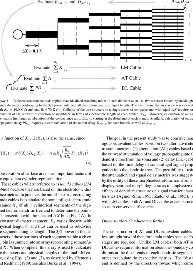
Figure 1. Cable construction methods applied to an idealized branching tree with stem diameter=10µm, five orders of branching and daughter branch diameters conforming to the 3/2 power rule, and all electrotonic paths of equal length. The electrotonic distance scale was calculated with Rm=10,000Äcm2and Ri=70Äcm. Collapse of the tree structure to a single series of compartments with equal1X requires only
evaluation of the outward distribution of membrane in terms of electrotonic length of each branch, Xi,j. However, calculation of outward
attenuation first requires tabulation of the conductance ratio, Bout,i,j, starting at the distal end of each branch. Similarly, calculation of outward
propagation delay PDi,jrequires inward tabulation of the output delay Dout,i,j, for each branch, as well as Bout,i,j.
as a function of Xj, S(Xj), is also the same, since
S(Xj)=π`(Xj)Deq(Xj)=π1X s Rm 4Ri Deq(Xj) 3 2. (4) Conservation of surface area is an important feature of the equivalent cylinder representation.
These cables will be referred to as lamda cables (LM cables) because they are based on the electrotonic dis-tance metric. In practice, the initial step in constructing lamda cables is to tabulate the somatofugal electrotonic distance Xj of all j cylindrical segments of the
digi-tized neuron dendritic tree and to determine the points of intersection with the selected1X bins (Fig. 1A). In a constant diameter segment, Xj varies linearly with
physical length`j and thus can be used to subdivide
the segment along its length. The 3/2 power of the di-ameter of those portions of each segment within a given Xjbin is summed into an array representing
somatofu-gal X . When complete, this array is used to calculate the diameters and physical lengths of the final LM ca-ble, using Eqs. (2) and (3), as described by Clements and Redman (1989; see also Burke et al., 1994).
The goal in the present study was to construct anal-ogous equivalent cables based on two alternative elec-trotonic metrics: (1) attenuation (AT) cables based on the outward attenuation of voltage propagating into the dendritic tree from the soma and (2) delay (DL) cables based on the time delay of somatofugal signal propa-gation into the dendritic tree. The possibility of using the attenuation and signal delay metrics was suggested by the utility of these morphoelectrotonic transforms to display neuronal morphologies so as to emphasize the effects of dendritic structure on signal transfer charac-teristics (Agmon-Snir, 1995; Zador et al., 1995). As with LM cables, both AT and DL cables are constructed so as to conserve surface area.
Dimensionless Conductance Ratios
The construction of AT and DL equivalent cables is less straightforward than for lamda cables because four stages are required. Unlike LM cables, both AT and DL cables require information about the boundary con-ditions at the distal ends of each dendritic segment in order to tabulate the respective metrics. The “distal” end is defined by the direction toward which current
flows within the segment. In the case of current flow-ing from the soma into the dendrites, the process of cable construction begins at the terminations of each dendritic path (Figs. 1B and 1C). Both AT and DL ca-bles require the value of the dimensionless conductance ratio Boutat the distal end of each cylindrical
compart-ment (Rall, 1977):
Bout =
Gout
G∞, (5)
where Gout is the conductance for current flowing out
of its distal end and G∞is the conductance of a semi-infinite extension of a cylinder with the same diameter d:
G∞= πd
3/2 2√RmRi
. (6)
The initial value of Bout is defined for terminating
segments by the assumed boundary condition, which in the present work was “sealed end” (Bout =0).
Cal-culation of the dimensionless input conductance Bin,i
at the other end of each cylindrical segment Bin,i=
Bout,i+tanh(Li)
1+Bout,itanh(Li)
, (7) where Liis the electrotonic length of that segment. The
Bout,i−1of the next more proximal cylinder i−1 is then Bouti−1=Bini · di di−1 ¸3/2 , (8) where di−i and di are the diameters of the respective
cylinders. The process is iterated toward the soma until a branch point is encountered, whereupon the iteration begins at the termination of the other daughter branch of that branch point. The dimensionless output conduc-tance of the parent branch Bout,pardepends on the input
conductances and diameter ratios of its two daughter branches:
Bout,par=Bin,dau1
· ddau 1 dpar ¸3/2 +Bin,dau 2 · ddau 2 dpar ¸3/2 . (9) In the present work, the Bout,jvalues were tabulated for
all segments of the digitized dendritic tree.
These conductance ratios, introduced by Rall (Rall, 1959, 1977), can be used to calculate the steady-state input conductance at any point in a branched tree,
including trees with arbitrary branch characteristics and nonuniform membrane properties (Fleshman et al., 1988). The values of Binfor the stem segments of all
trees belonging to the neuron are summed to give the input conductance into the entire dendritic tree. This sum is added to the soma conductance to give the total input conductance of the neuron (see Fleshman et al., 1988).
Attenuation Cables
The steady-state voltage attenuation atten in a mem-brane cylinder (i.e., having constant diameter) depends on its electrotonic length L and the boundary condition, Bout, at the end distal to the direction of current flow
(Rall, 1959, 1977): atten= Vin
Vout =
cosh(L)+Boutsinh(L), (10)
where Vinand Voutare the steady-state voltages at the
proximal and distal ends of the cylinder. Note that atten is always>1.0. The attenuation metric actually used for cable construction was A= ln(atten), as in earlier work (Agmon-Snir, 1995; Zador et al., 1995). With the tabulated Boutvalues for the entire dendritic
tree, calculation of outward (somatofugal) A can begin at the soma using Eq. (10) and then progress outward (i.e., in the direction of current flow; see Fig. 1) adding the values along the j th path to its termination, such that Aj= n X k=1 ln(attenk)= n X k−1 Ak, (11)
where the index k refers to all n segments on the direct path from the soma up to and including its termination segment.
The primary objective was to construct an equiva-lent cable that conserves the surface area of the original branched tree as in LM cables but distributed accord-ing to the outward attenuation Aj in the original tree.
Unfortunately, the tabulated Ajvalues for segments in
the branched tree cannot be used in the same way as Xj
in constructing LM cables because Aj is a nonlinear
function of physical segment length. The strategy to overcome this problem was to divide each segment in the tree into small increments of physical length (5µm was used in the present work) that can each be regarded as piecewise linear with respect to Aj. The values of Aj
used to calculated the location of each increment in the sequence of1A bins selected for the cable. The d3/2 and surface area for the increment were then summed into the appropriate1A bin or proportionately to ad-joining bins if the fragment crossed a bin boundary. This process was iteratively applied to each of the seg-ments in the branched tree until the final cable array contained the summed d3/2 and surface areas for the entire dendritic tree, distributed into1A bins exactly as found in the original tree(s).
The 2/3 root of the summed d3/2gave a provisional physical diameter D∗for each cable compartment (see Eq. (2)). The physical length of the compartment was then calculated from the summed area value S(1An).
The actual ln(atten) of the1A compartments in this “raw” cable array often did not exactly match the de-sired1A. Therefore, a successive approximation pro-cedure was used to adjust the physical lengths and di-ameters of each compartment in order to produce the exact1A, while maintaining the area of each compart-ment at its original value. Because of the dependence on boundary conditions, this process began with the terminal compartment, where Bout =0. The1A∗ of
the terminal compartment was calculated from its S and D∗values, as in the process for the full tree (Fig. 1B). The normalized difference between 1A∗j and the desired1A—
diff =1A ∗
j−1A
1A (12) —was multiplied by an appropriate weighting factor (usually 0.1, chosen to ensure convergence) in order to adjust the compartment’s length and diameter, dividing the length and multiplying the diameter to maintain the area constant. The process was iterated until1A∗j and
1A differed by² <0.001. With the correct dimensions in the terminal cable compartment, the process was iterated for successively more proximal compartments until all had the desired1A.
Delay Cables
The process of calculating the delay cable for a partic-ular structure was the same four-stage process used for attenuation cables, but the metric used was the propaga-tion delay (PD), which is a measure of the time delay (in ms) of propagation of the centroid of any transient volt-age within a membrane cylinder (Agmon-Snir, 1995). It is important to note that Cm must also be specified
because the PD transform depends on the membrane
time constant,τ =RmCm, as well as on the output
con-ductances. Like A, PD varies nonlinearly with physical distance along each cylindrical compartment and the solution to this problem was the same as detailed for the AT cable construction. The only difference (other than the equations used) was that the necessary boundary conditions also include the output delay Dout, which
is the time domain analog of the steady-state output conductance Bout. In any given membrane cylinder,
PD depends on its electrical length L, the local mem-brane time constant τ = RmCm, its output
conduc-tance (represented by Bout), and its output delay Dout
(Agmon-Snir, 1995). Some of the equations using in the present work (Eqs. (14) and (15)) were modified from those given by Agmon-Snir (1995, his Eq. (36)) in order to utilize the dimensionless conductance ratios already calculated.
Analogous to the AT cables, the first step was to tabulate values for Dout and Bout for each cylinder
in the original branched structure, starting with the terminations of each dendritic path (Fig. 1C). Val-ues of Doutwere obtained with the following equation
(Agmon-Snir, 1995, his Eq. (35)):
Dout=τ · 1 2 +2 κ(1+ξ)−ξL ξ2exp(−2L)−exp(2L) ¸ (13)
for a terminal compartment with sealed end where Bout = 0, κ = 0, and ξ = 1. For each more
prox-imal compartment κ = Bout £1 2− D∗out τ ¤ Bout+1 , (14) where Dout∗ is the output delay of the immediately distal compartment and
ξ =1−Bout
1+Bout
. (15)
The process was iterated for all paths in the dendritic tree, using Eqs. (7) to (9) as well as those above.
Using the tabulated values, calculation of the out-ward propagation delay PD began at the somatic end of the tree (Fig. 1) using the following equation (Agmon-Snir, 1995, his Eq. (37)):
PD=τ · [ξ +1]κ−ξL ξ +exp[2L] −κ+ L 2 ¸ . (16)
These values were tabulated for each segment in the tree and their sum was accumulated along each path to a dendritic termination. Since PD, like A, is a non-linear function of physical length along each segment in the tree, the distribution of Pd(1PDn)3/2 and
P
S(1PDn) into the 1PDn bins of the cable array
was done using short pieces of the successively more distal segments of the tree in the same way as done for the AT cables. Again, the1PD of compartments of the raw cable array usually did not exactly match the target
1PD desired. Therefore, the same process of succes-sive approximation was used to adjust the lengths and diameters of each cable compartment in order to match the target1PD. In the resulting delay cable, each final compartment has the appropriate 1PD and the same surface area as the original components of the dendritic tree with that somatofugal PD.
Additional Attributes
The computer program that was written to implement the above procedures also calculated the input conduc-tance into the original dendritic tree(s) of the anatom-ical neuron data file, using specified values for Rm,
Ri, and Cm(1.0µF/cm2 in the present work). It also
generated two output files, one of which encoded the structure of the desired equivalent cable for import into the neuron simulation package, NODUS (De Schutter, 1992), that was used for testing the transient behav-ior. The other file contained the dimensions of cable compartments, their actual 1X , 1A, and 1PD val-ues, the cumulative somatofugal values for the same metrics, and the cumulative area and physical length of the cable (e.g., Figs. 2 and 3). It was of particular importance to ensure that the effective surface area of the soma was the same for full and cable models of the same cell. NODUS calculates this by subtracting the cross-sectional areas of all stem dendrites arising from the soma from the surface area implied by the specified soma diameter. This effect of different stem areas in the full cell cable models was taken into account in the program. This source code, written in Pascal for the Macintosh, is available from the author on request.
Test Criteria
The object of this work was to compare the steady-state input conductance and transient responses of mod-els with fully branched dendrites with modmod-els that incorporate their equivalent cables plus a soma of the
same dimensions as the full model, all constructed us-ing the same values for Rm, Cm, and Rj. Transient
responses to identical brief current pulses at the model soma produced by the equivalent cable models were compared with those generated by the fully branched model, using relatively small values of 1X (≤0.07) for the latter. Transients were calculated using the Fehlberg (exact) integration method with adaptive time steps.
The percentage “error” between the cable and full model transients, Verr(t), was calculated as a function
of time by Verr(t)= · Vcbl(t) Vfull(t) −1 ¸ 100, (17)
where Vcbl(t)and Vfull(t)are the transients produced by
the cable and full models, respectively (e.g., Figs. 4A and 4C). The difference between the transients re-sponses produced by the full model and the different cable representations at1t =0.1 ms were also evalu-ated by calculating the RMS error:
RMSerr(ti)=
sPi=max
i=minVerr(ti)2
count , (18)
where count is the number of values already summed to the time step in question. For any given time epoch, the RMS error gives a single value summation of the disparity between the V(t)curves produced by cable models in relation to the full structure. It was also use-ful to examine the evolution of the RMS error during the time course of the transients. This was done back-wards in time from a point at which the curves had converged to near zero error (“back RMS error”; see Figs. 4B and 4D), which gives a clear impression of the relative fidelity of the different models over the tran-sient time course. For any given time epoch, the value of RMSerr(t)was the same whether it was calculated forward or backward in time.
Results
Idealized Tree Structure
The algorithms for cable construction were first applied to the idealized tree structure shown in Fig. 1, using Rm=10,000 Äcm2, Ri=70 Äcm,
and Cm=1.0 µF/cm2 as parameters. This tree had
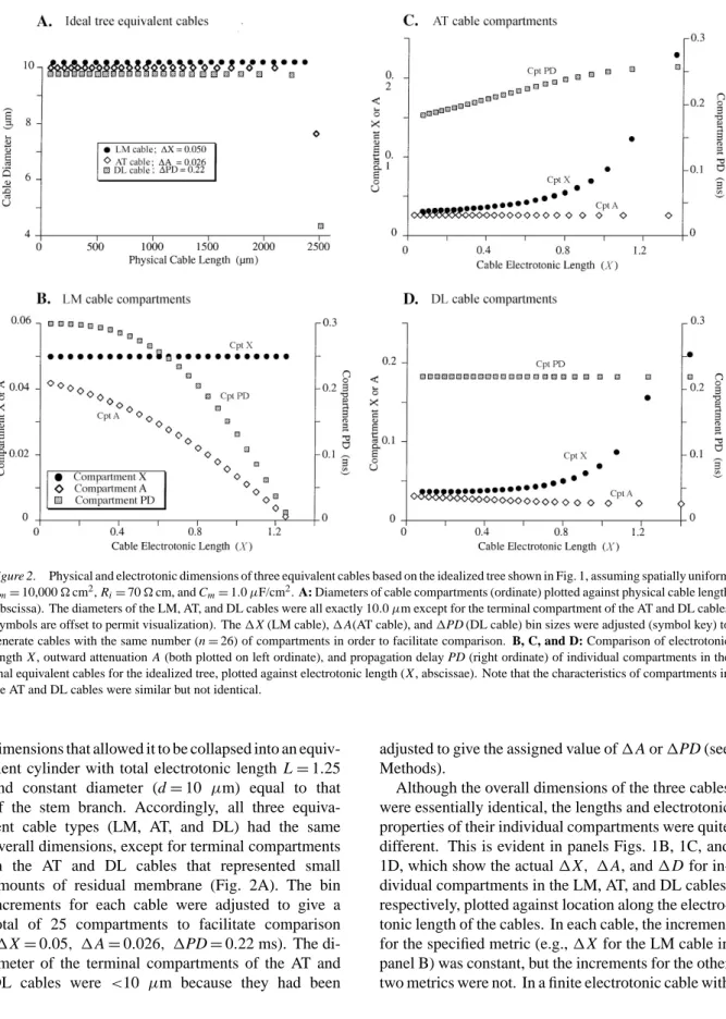
Figure 2. Physical and electrotonic dimensions of three equivalent cables based on the idealized tree shown in Fig. 1, assuming spatially uniform
Rm=10,000Äcm2, R
i=70Äcm, and Cm=1.0µF/cm2. A: Diameters of cable compartments (ordinate) plotted against physical cable length
(abscissa). The diameters of the LM, AT, and DL cables were all exactly 10.0µm except for the terminal compartment of the AT and DL cables (symbols are offset to permit visualization). The1X (LM cable),1A(AT cable), and1PD (DL cable) bin sizes were adjusted (symbol key) to
generate cables with the same number (n=26) of compartments in order to facilitate comparison. B, C, and D: Comparison of electrotonic length X , outward attenuation A (both plotted on left ordinate), and propagation delay PD (right ordinate) of individual compartments in the final equivalent cables for the idealized tree, plotted against electrotonic length (X , abscissae). Note that the characteristics of compartments in the AT and DL cables were similar but not identical.
dimensions that allowed it to be collapsed into an equiv-alent cylinder with total electrotonic length L=1.25 and constant diameter (d=10 µm) equal to that of the stem branch. Accordingly, all three equiva-lent cable types (LM, AT, and DL) had the same overall dimensions, except for terminal compartments in the AT and DL cables that represented small amounts of residual membrane (Fig. 2A). The bin increments for each cable were adjusted to give a total of 25 compartments to facilitate comparison (1X=0.05, 1A=0.026, 1PD=0.22 ms). The di-ameter of the terminal compartments of the AT and DL cables were <10 µm because they had been
adjusted to give the assigned value of1A or1PD (see Methods).
Although the overall dimensions of the three cables were essentially identical, the lengths and electrotonic properties of their individual compartments were quite different. This is evident in panels Figs. 1B, 1C, and 1D, which show the actual1X, 1A, and1D for in-dividual compartments in the LM, AT, and DL cables, respectively, plotted against location along the electro-tonic length of the cables. In each cable, the increment for the specified metric (e.g.,1X for the LM cable in panel B) was constant, but the increments for the other two metrics were not. In a finite electrotonic cable with
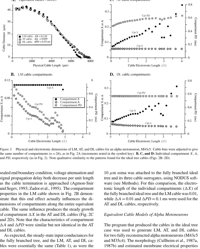
Figure 3. Physical and electrotonic dimensions of LM, AT, and DL cables for an alpha motoneuron, M43c5. Cable bins were adjusted to give the same number of compartments (n=26), as in Fig. 2A (increments noted in the symbol key). B, C, and D: Individual compartment X,A,
and PD, respectively (as in Fig. 2). Note qualitative similarity to the patterns found for the ideal tree cables (Figs. 2B–2D).
sealed end boundary condition, voltage attenuation and signal propagation delay both decrease per unit length as the cable termination is approached (Agmon-Snir and Segev, 1993; Zador et al., 1995). The compartment properties in the LM cable shown in Fig. 2B demon-strate that this end effect actually influences the di-mensions of compartments along the entire equivalent cable. The same influence produces the steady growth of compartment1X in the AT and DL cables (Fig. 2C and 2D). Note that the characteristics of compartment
1A and1PD were similar but not identical in the AT and DL cables.
As expected, the steady-state input conductances for the fully branched tree, and the LM, AT, and DL ca-bles were essentially the same (Table 1), as were the transient decays following a brief somatic current pulse (10 nA, 0.3 ms duration). For transient simulations, a
10µm soma was attached to the fully branched ideal tree and its three cable surrogates, using NODUS soft-ware (see Methods). For this comparison, the electro-tonic length of the individual compartments (1X ) of the fully branched ideal tree and the LM cable was 0.01, while1A=0.01 and1PD=0.1 ms were used for the AT and DL cables, respectively.
Equivalent Cable Models of Alpha Motoneurons The program that produced the cables in the ideal tree case was used to generate LM, AT, and DL cables for two fully reconstructed alpha motoneurons (M43c5 and M35c4). The morphology (Cullheim et al., 1987a, 1987b) and estimated membrane electrical properties (Fleshman et al., 1988; Segev et al., 1990) of both cells have been published. Motoneuron M43c5 had
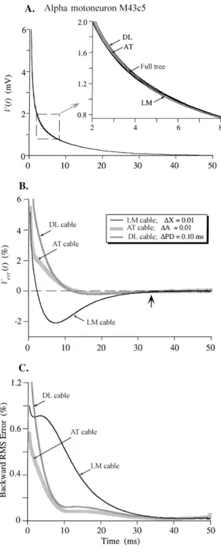
Figure 4. Plots of the disparity between transient responses pro-duced in the full cell model versus in three equivalent cable mod-els of an alpha motoneuron (cell M43c5). Parameters for transient simulations are given in the text and the cable increments used are indicated in the symbol key in B. A: Plots of V(t)obtained from the fully branched cell model (heavier line) and for the three cable surrogates. The largest disparities were evident between 2 and 8 ms, as depicted in the inset. B: Verr(t)curves showing the percent error
11 dendrites, with a total of 163 paths that termi-nated between X=0.4 and X=2.8 (median about 1.4), assuming Rm=11,000Äcm2, Ri=70Äcm, and
Cm=1.0µF/cm2 (Fleshman et al., 1988). Assuming
a spherical soma with the average diameter measured for this cell, the ratio of dendritic to somatic membrane area, Adend/Asoma (609,807 and 7,481µm2,
respec-tively), was 81.5.
The physical dimensions of the three equivalent ca-bles for cell M43c5 (Fig. 3A) illustrate the marked contrast between cables for an actual motoneuron and those for an idealized tree (cf. Fig. 2A). The diameters of each of the surrogate cables were roughly constant only in the proximal one-fourth and then fell more-or-less linearly to their terminations (see also Fig. 9 in Fleshman et al., 1988). The AT and DL cables differed from the LM cable mainly in their most distal portions. For purposes of illustration (as in Fig. 2A), the cable bin increments were adjusted to produce cables with 26 compartments in each case. The graphs of cumula-tive area as a function of cable length were curvilinear and closely similar for all three cables (not shown). The patterns of1X, 1A, and1PD for individual compart-ments in relation to electrotonic location (Figs. 3B–3D) were basically similar to the idealized tree (Figs. 2B– 2D), allowing for the irregularities introduced by the variety of electrotonic path lengths in the real neuron. The steady-state input conductance of the entire den-dritic tree of this cell was most closely matched by the AT cable surrogate (Table 1; error=0.04%).
Because of the large size of this motoneuron and its relatively low estimated Rm, 1X=0.07 was used
to represent the cell for transient simulation. This pro-duced a model cell with 2,664 compartments, which is near the maximum capacity for NODUS. The fully branched dendrites were connected to a spherical soma with diameter of 48.8 µm, in which a 30 nA, 0.3 ms pulse was delivered at t=0. The resulting decay tran-sient was compared with trantran-sients generated by the
between the transients produced by each cable and that of the fully branched model (see Methods). Note that AT and DL cable transients converged near zero error well before that of the LM cable response but all error curves eventually converged to zero error at about three times the membrane time constant (arrow). C: Backward RMS error curves (RMSerr(t); see Methods) calculated from the end of the transient simulations (50 ms) down to 0.4 ms (backward error) for the responses shown in A. Note that the curves for AT and DL cables exhibited much lower RMS error than that for the LM cable for most of the time courses. The AT cable was slightly more accurate than the DL cable.
Table 1. Comparison of summed input conductance for full tree and equivalent cable models.
Ideal tree M43c5 M35c4 GMN 9118
Gin Error Gin Error Gin Error Gin Error
Model (nS) (%) (nS) (%) (nS) (%) (nS) (%)
Full tree 50.37 — 382.87 — 121.73 — 25.49 —
LM cable 50.37 0 388.30 1.41 124.67 2.41 26.21 2.82 AT cable 50.36 −0.02 382.75 −0.03 121.68 −0.04 25.48 −0.04 DL cable 50.36 −0.02 377.11 −1.50 120.72 −0.83 25.51 0.08
same pulse in each of the three types of equivalent ca-bles connected to a soma with the same effective sur-face area (see Methods) and the increments given in the symbol key in Fig. 4B.
The curves in Fig. 4A illustrate the V(t)decay tran-sients produced by the fully branched cell model and the LM, AT, and DL surrogate models. The inset shows the relatively small differences between the curves within the dashed line box in more detail. It is difficult to evaluate the relative fidelity of the cable models from such a display. However, they are magnified in plots of the instantaneous error, Verr(t), between the decay
transient from the full cell and those from the three cable models, evaluated from 0.4 to 50 ms (Fig. 4B; see Eq. (17)). The errors were relatively large imme-diately after the simulated current pulse (t=0.4 ms), but each curve eventually converged to near zero er-ror by about t=33 ms (arrow; three times theτ0 of 11 ms). Thus the longest time constants,τ0(in this case
τ0=τm=RmCm=11 ms) were identical in all four
structures, but the shorter equalizing time constants that represent the spread of current into the dendrites were clearly not the same. The AT cable appeared to mimic the mixture of equalizing time constants in the full tree better than the DL or LM cables.
Because of the disparity in shapes between the Verr(t)curves, it proved to be useful to evaluate the
rel-ative errors by calculating the RMSerr(t)backwards in time from a point at which all of the error curves had converged to near zero (Eq. (18); see Methods). Figure 4C illustrates backward RMSerr(t)curves for the three cables, calculated from 50 ms down to 0.4 ms. Viewed in this way, the LM curves clearly showed the largest error down to about 2 ms, when the RMSerr(t) for the DL curve became larger. The AT cable had the lowest RMSerr(t)throughout. The total RMS errors accumulated between 2 ms and 33 ms (3×τ0;about
Table 2. Simulations with spatially uniform Rm.
M43c5 M35c4 GMN9118 Rm 11,000 20,000 33,000 ρ(uniform Rm) 56.3 29.9 28.3 Adend/Asoma 81.5 45.1 35.6 RMS err (3τ) LM (%) 1.12 1.30 2.36 RMS err (3τ) AT (%) 0.64 0.69 0.88 RMS err (3τ) DL (%) 1.09 0.98 0.75
where the three curves converged) for the three cable models of this cell are given in Table 2. The value of 2 ms was chosen to start this calculation because, in practice, the first 1 to 2 ms of experimental transient records are usually ignored because they are often con-taminated by artifacts.
Similar results were obtained with another alpha mo-toneuron, a type S soleus motoneuron with estimated Rm=20,000 Äcm2 (cell M35c4; Fleshman et al.,
1988). Although this cell had a simpler dendritic tree than M43c5, the transient error comparisons were simi-lar in shape and magnitude to those illustrated in Fig. 4. In this case, the Verr(t)curves converged to near zero at
about t=60 ms, again about three timesτm=20 ms.
As with M43c5, the AT cable showed the smallest error during transients as evaluated by backward RMSerr(t) curves as well as by total RMS error (Table 2). The AT cable also best matched the total input conductance of the fully branched dendritic tree (error 0.04%; Table 1). Cable Models of a Gamma Motoneuron
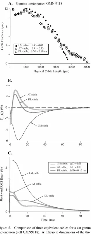
The final example is a gamma-motoneuron that has been described in detail anatomically (cell GMN9118; Moschovakis et al., 1991) and electrophysiologically (Burke et al., 1994). This cell had a dendritic tree that
Figure 5. Comparison of three equivalent cables for a cat gamma motoneuron (cell GMN9118). A: Physical dimensions of the three equivalent cables, as in Figs. 2A and 3A. Cable increments were again adjusted to produce the same number of compartments (n=26); increments given in the symbol key. B: Verr(t)for 90 ms transient responses using spatially uniform Rm=33,000Äcm2, Ri=70Ä
cm, and Cm=1.0µF/cm2;cable increments for simulations given
in symbol key in C. Note that the error curves converged near zero only after 90 ms (about three times the system time constant of
was much smaller and simpler than either of the alpha motoneurons discussed above (nine dendrites with a total of 33 terminating paths). The ratio of dendritic to somatic membrane area (105,382 and 2,961µm2, re-spectively) was smaller than in the alpha motoneurons (35.6; Table 2). With an estimated Rmof 33,000Äcm2,
these paths ended between X=0.6 and X=1.4 (as before, Ri=70 Äcm and Cm=1.0 µF/cm2). The
dimensions of the AT and DL cables for this cell showed considerable differences from the LM cable over most of the distal two-thirds (Fig. 5A; cf. Fig. 3A). As in the other examples, the total steady-state input conductance into the dendrites of the AT cell model most closely matched that of the fully branched cell (Table 1).
Transients in the full cell were simulated in a model with 2,367 compartments (1X=0.01)and a spherical soma with diameter=30.7µm. The instantaneous er-rors, Verr(t), between the cable transients and the fully
branched tree were quite large for the LM in compari-son with the AT and DL cables (Fig. 5B) but all three curves converged to near zero error at t∼90 ms (ap-proximately three timesτ0=33 ms). Evaluation of the backward RMS error from 90 ms (Fig. 5C) showed that the LM model produced the largest cumulative er-ror throughout the duration of the transients, while the AT cable outperformed the DL cable for times>10 ms from the onset. The total RMS error over 2 to 90 ms of the transient was smallest for the DL cable, only slightly higher for the AT, and quite a bit larger for the LM cables (Table 2).
Effect of Reducing Cable Compartment Number The comparisons discussed above were done using equivalent cables with small increments of the mor-phoelectrotonic metrics (e.g.,1X=0.01), in order to minimize errors due to the assumption of compart-ment isopotentiality (see Segev et al., 1998). How-ever, one objective of equivalent cable representa-tions is to reduce the complexity of dendritic neurons in order to enhance computational efficiency (Segev, 1992; Douglas and Martin, 1992; Bush and Sejnowski, 1993). Accordingly the effect of increasing the morphoelectrotonic bin size (i.e., using increasingly
33 ms), as in the responses from alpha motoneuron models shown in Fig. 4. C: Backward RMS error (90 ms down to 0.4 ms), showing that the AT and DL cables outperformed the LM cable over most of the transient duration.
coarse cables) in the three types of cable models was examined.
Figure 6 illustrates families of backward RMS er-ror curves for increasingly coarse representations of cell M43c5. In each case, increasing the cable com-partment size over an order of magnitude produced relatively small reductions in transient fidelity; seri-ous increases in errors were found only when there was a 20-fold increase in bin size. Paradoxically, the coarsest LM cable exhibited slightly smaller back-ward errors in comparison with those having smaller values of1X . Reducing the number of model com-partments markedly decreased computation time for transient simulations. These results demonstrate that relatively coarse equivalent cables, when properly con-structed, can provide rather good fidelity with the fully branched model.
Effect of a Somatic Shunt
Recent evidence suggests that the use of sharp micro-electrodes may introduce somatic shunt conductances (Spruston and Johnston, 1992; Staley et al., 1992) that greatly complicate the interpretation of electrotonic behaviors (Durand, 1984; Iansek and Redman, 1973; White et al., 1992). A somatic shunt was simulated in the present work by decreasing the value of Rm,somafor
transient simulation runs in NODUS (Fleshman et al., 1988).
Transient responses produced by the ideal branch-ed tree in Fig. 1A and its cable surrogates (Fig. 2) were examined with Rm,soma=500Äcm2and
Rm,dendrite=10,000Äcm2. All of the cable responses
were very closely similar to each other as well as to that of the full tree structure, except that the system time constantτ0 in all cases was 9.45 ms, rather than 10 ms for the uniform Rmcase. This orderly behavior,
entirely expected for an idealized tree, was not found with real neurons. In order to compare the results in different motoneurons, the ratio of dendritic to somatic local time constants β was maintained constant (see Rall et al., 1992).
Figure 7 illustrate Verr(t) curves for alpha (panel
A) and gamma (panels B and C) motoneurons already presented in Figs. 4 to 6, using the same Rm,dendritesas
in the previous simulations but with Rm,somaadjusted
to produceβ=66 (Table 3). In the presence of a so-matic shunt, the errors between the transients produced
Figure 6. Backward RMS error curves for the three cable types based on cell M43c5, showing the effect of making the cables more coarse by increasing the compartment bin sizes. Increasing bin size over a tenfold range produced little degradation in transient fidelity, but a further increase to 20 times the minimum size showed a large error. Cable increments and the resulting number of compartments in each cable (n) are indicated for each curve.
Figure 7. Instantaneous error curves produced by cables with nonuniform Rm(adding a somatic shunt). A and B: Verr(t)curves
for cells M43c5 (A) and GMN9118 (B) when the somatic membrane resistance Rm,somawas reduced in each model from the spatially
uni-form values used in Figs. 4 to 6 to Rm,soma=167 and 500Äcm2,
respectively (see Table 3). See text for full discussion. C: V(t)curves from the full cell model of GMN9118 compared to that of the LM cable for the same cell, both with Rm,soma=500Äcm2. This
illus-trates the largest disparity found in the present work.
Table 3. Somatic shunt simulations.
M43c5 M35c4 GMN9118 Rm,dendrites 11,000 20,000 33,000 Rm,soma 167 303 500 β 66 66 66 ρ(shunt) 0.85 0.45 0.43 RMS err (3τ) LM (%) 2.19 2.87 4.96 RMS err (3τ) AT (%) 2.05 1.85 2.04 RMS err (3τ) DL (%) 3.53 2.81 2.15
by the fully branched and the cable models were both larger and had more complex time courses than the cases examined with uniform Rm. In particular, none
of the error curves converged to zero error, and none settled to the same system time constantτ0as the full cell model (i.e., none of the curves became parallel to the abscissa; see Figs. 4B and 5B). As was the case with spatially uniform Rm, the Verr(t)curves of the AT
and DL cables resembled one another, but the error tra-jectories for the LM cables were quite different. The results with the third alpha motoneuron M35c4 were similar to those found for M43c5 (see Table 3). In or-der to put the percent errors plotted in these curves into perspective, the V(t)transient from the full model of cell GMN9118 is shown in Fig. 7C superimposed on the transient produced by the LM cable model for that cell, both with the same somatic shunt. The two transients cross and recross in several places (arrows), an effect much more obvious in the LM error curve in panel B. Despite the larger errors, the AT cable models outper-formed the other two even in the presence of a somatic shunt.
Discussion
This article demonstrates that it is possible to col-lapse arbitrarily complex dendritic trees into equiva-lent cables based on outward voltage attenuation and on outward signal propagation delay, which to my knowledge have not previously been used as bases for construction of cable surrogates. In addition, the AT and DL equivalent cables outperform LM cables in mimicking the steady-state input conductances and transient responses of fully branched models of actual motoneurons whether or not Rm is spatially uniform.
This greater fidelity presumably results from the fact that the construction of AT and DL cables take into account the end effects of terminating dendritic paths (Agmon-Snir, 1995; Agmon-Snir and Segev, 1993; Zador et al., 1995), which do not enter at all into the construction of LM cables that are based only on somatofugal electrotonic distance (Clements and Redman, 1989). The input conductances of AT cables based on actual motoneurons were virtually the same as those of the full branched structures (Table 1), which suggests that AT cables more accurately mimic the steady-state voltage distribution within the full model than the other cable types.
Why Do Errors Appear in Cable Simulations of Neuronal Dendritic Trees?
All three types of equivalent cables produced from the ideal dendritic tree (Figs. 1 and 2) showed input con-ductances (Table 1) and transient responses that were essentially identical to those of the fully branched struc-ture and therefore to each other. This could hardly have been otherwise because all of these cables had the same diameter and total length, except for the terminal compartments that represented small amounts of resid-ual membrane left after segmentation of the branched tree according to1AT or1D L (Fig. 2A). The ideal case was used to validate the present computational strategy.
The situation was different in the case of actual mo-toneurons with spatially uniform Rm. With respect to
fidelity of the transient responses, the AT cables were marginally superior to the DL cables over much of the transient durations but both showed some residual er-ror, albeit less than the LM cables (Figs. 4 and 5). As Rall has shown (Rall, 1969), the transients responses at any location x, in an electrotonic cable structure, branched or unbranched, can be represented as the sum of a series of exponentials: V(x,t)=V∞(x,t)− nmax X n=0 Cnexp(t/τn), (19)
where Cn are coefficients, or weights, that control the
magnitude of each time constant’s (τn) contribution to
the net response and V∞(x,t)is the steady-state trans-membrane voltage. For a continuous cable nmax= ∞
while in a compartmental simulation, nmax equals the
number of compartments and the values of Cnandτn
can be obtained from the eigenvalues of the simulation matrix (see Rall et al., 1992). Therefore, models with
different numbers of compartments must have differ-ent mixtures of Cnandτn, which may or may not
sum-mate into similar net responses (e.g., Rall et al., 1992, their Fig. 7). In the case of fully branched motoneu-rons with spatially uniform Rm, they did not (Figs. 4
and 5), although the Verr(t)curves for the
motoneu-rons converged near zero error as time increased to about three timesτ0. This indicates thatτ0 was iden-tical in branched and cable models, as expected when the same values of Rmand Cm apply to all regions of
branched and cable models of a given cell. The larger errors at earlier times presumably resulted from differ-ences in the mixture of shorter time constants and/or their coefficients.
The fact that the relative fidelity of equivalent cable transients showed little degradation as the number of compartment decreased (up to a point; see Fig. 6) in-dicates that the number of coefficient–time constant pairs per se is not critical. In fact, Verr(t) actually
decreased slightly in LM cable responses as1X in-creased (Fig. 6A). The errors in transients produced by the present equivalent cable models must result from the inability of these reduced cables (and possibly of any reduced cable model) to accurately reproduce all of the end effects and reflection terms that are inherent in a natural branched dendritic tree. The AT and DL cables, do a better job than the LM cables, but they are not perfect.
Recently, an equivalent cable formulation that takes account of all of the electrotonic pathways within a tree structure was introduced (Ogden et al., 1999; Whitehead and Rosenberg, 1993). Such a structure in principle should provide an exact match for the elec-trical behavior of the tree as observed from any point within it. Preliminary results using simple asymmet-rical trees, attached to a small soma and treated ex-actly as described in this article, showed that tran-sient responses of such “Lanczos” equivalent cables were virtually identical with those from the branched structure (R.E. Burke and J.M. Ogden, unpublished ob-servations). However, the “Lanczos” equivalent cable can require many thousands of compartments to repre-sent each current path in the structure, thus providing no structural simplification even for modestly complex real trees.
Transients in Models with Simulated Somatic Shunt The introduction of a simulated passive shunt con-ductance in the soma complicates neuron models be-cause the soma then has a shorter effective local time
constant than the dendrites (Durand, 1984; Iansek and Redman, 1973). The slowest time constantτ0 in the somatic transient response to a short current pulse (sometimes called the system time constant; Fleshman et al., 1988) is somewhere betweenτsoma=Rm,somaCm
andτdendrites=Rm,dendritesCm (assuming spatially
uni-form Rm,dendrites). When Rm is the same throughout
the neuron, equalizing currents flow out into the den-drites after a somatic voltage perturbation until all of the membrane capacitance is equally charged, after which transmembrane voltage eventually decays everywhere at the same rate, which is the membrane time constant,
τm=RmCm, which occurs at t≥3τ0(Figs. 4 and 5). Initial somatofugal equalizing currents also flow during and after a voltage perturbation in a soma with a local shunt conductance. However, because the somatic ca-pacitance discharges more rapidly than the dendritic, equalizing currents soon begin to flow back toward the soma from regions with longer local time constants even as the more distal dendritic regions continue to be charged (Fleshman et al., 1988). The cell interior returns to an isopotential state only when all of the in-jected charge has completely dissipated. The sensitivity of the Verr(t)curves used in the present work reveals
the complexity of this process, which is not usually appreciated.
Because the soma receives dendritic current during the process of charge dissipation, its potential decays at a rate somewhere betweenτsomaandτdendrites. The
value ofτ0 in model of an ideal cylinder attached to spherical soma with a shunt conductance depends on the electrotonic length of the cylinder, L, β, and the value ofρ in the absence of a somatic shunt (Holmes and Rall, 1992). In the present ideal tree models with Rm,soma=500 Äcm2 and β=20, τ0 recorded in the soma was 9.45 ms in the full tree and all its cable sur-rogates, entirely compatible with the calculations of Holmes and Rall. It was therefore surprising that the Verr(t)curves for equivalent cable models of actual
mo-toneurons did not converge to the sameτ0as the full cell model (Figs. 7A–7C), as found for the uniform Rm
models (Figs. 4 and 5).
It is important to recall that the somatic, dendritic, and total membrane areas of each fully branched cell and its equivalent cables were the same in all of the models used for transient simulation. This proved to be a critical factor in the presence of somatic shunts; small discrepancies in effective somatic area produced larger errors. Given that the respective local time con-stants were also the same, one would expect that τ0 would be the same for all models of a given cell, as
was found for the ideal tree. In contrast, the sensitiv-ity of the Verr(t)curves revealed that the late voltage
decays of the cable model responses not only differed from the full tree but also differed from each other. Indeed, the Verr(t)curves for each cable model
contin-ued to exhibit curvature until numerical truncation er-rors made it impossible to evaluate them. Even in these noiseless simulations, no stableτ0was attained before the traces became too small to measure. It seems likely that this was also true of the full cell simulations. The spatiotemporal distribution of transmembrane voltage decay and the associated flows of equalizing currents in a fully branched neuron are complex in the presence of a somatic shunt and this also appears to be true in the cable surrogates. It seems important that the AT and DL equivalent cables mimic these factors more accurately than LM cables.
Are These Equivalent Cables of Useful in Neuron Modeling?
The primary purpose of the present work was to explore whether alternative morphoelectrotonic transforms can be used to reduce anatomically complex neurons into simple surrogate models that embody the electrotonic characteristics of the original cells more accurately than is possible in the LM cable formulation. The re-sults presented answer this question affirmatively. Rel-atively coarse AT and DL cables mimic the steady-state and time-domain behaviors of complex neurons relatively well and may therefore be of use in net-work models that utilize dendritic properties in netnet-work elements.
Such cables may also be useful in attempts to esti-mate specific membrane properties from morphologi-cal and electrophysiologimorphologi-cal data, which require time domain information (Rall et al., 1992). The possible presence of spatially nonuniform membrane proper-ties greatly complicates such efforts (Clements and Redman, 1989; Fleshman et al., 1988; White et al., 1992). Prediction of transient behavior in realistically complex model neurons with nonuniform Rm using
analytical methods is neither straightforward (Major et al., 1993) nor entirely free of anatomical com-promises (e.g., Evans and Kember, 1998; Poznanski, 1996). As a practical alternative, compartmental equiv-alent cables provide computationally efficient surro-gates for use in trial-and-error membrane parameter estimation procedures (Clements and Redman, 1989). Such step-wise approaches also provide a heuristically
satisfying way to explore sensitivity to changes in the various model parameters (Burke et al., 1994).
In recent years, various alternative approaches have been suggested to simplify the electrotonic architecture of neurons into equivalent cables, some for specific purposes (e.g., Bush and Sejnowski, 1993; Douglas and Martin, 1992; Stratford et al., 1989) and others as heuristically interesting objects (Ogden et al., 1999; Whitehead and Rosenberg, 1993). A recent extensive theoretical analysis suggests that collapsing real neu-rons into equivalent cables according to electrotonic metrics that conserve membrane area, as in the present work, are superior to some of these alternatives (Ohme and Schierwagen, 1998). The AT and DL cable mod-els discussed in this paper are specifically formulated to conserve the electrotonic distribution of membrane area. Construction of these cables, although seemingly complex (see Methods), is based on a straightforward premise that is easily understood. The program that generates them can reduce a digitized motoneuron with 700 to 1,000 compartments into an equivalent cable of any type in less than one second. The algorithm could easily be adapted to construct multicable “cartoon” representations of pyramidal neurons (Stratford et al., 1989). The new equivalent cable formulations not only reveal some interesting aspects of reduced neuron mod-els, but they also appear to be practical alternatives to existing schemes.
Acknowledgments
The author wishes to thank Dr. Idan Segev for discus-sions that initiated this work and Dr. Hagai Agmon-Snir for his helpful comments on the application of the propagation delay metric to the construction of PD cables.
References
Agmon-Snir H (1995) A novel theoretical approach to the analysis of dendritic transients. Biophys. J. 69:1633–1656.
Agmon-Snir H, Segev I (1993) Signal delay and input synchroniza-tion in passive dendritic structures. J. Neurophysiol. 70:2066– 2085.
Burke RE (1997) Equivalent cable representations of dendritic trees: Variations on a theme. Soc. Neurosci. Abstr. 23:654 (Abstr # 261.16).
Burke RE, Fyffe REW, Moschovakis AK (1994) Electrotonic ar-chitecture of cat gamma motoneurons. J. Neurophysiol. 72:2302– 2316.
Bush PC, Sejnowski TJ (1993) Reduced compartmental models of neocortical pyramidal cells. J. Neurosci. Meth. 46:159–166.
Clements J, Redman S (1989) Cable properties of cat spinal mo-toneurones measured by combining voltage clamp current clamp and intracellular staining. J. Physiol. (Lond.) 409:63–87. Clements JD (1986) Synaptic Transmission and Integration in Spinal
Motoneurones. Ph.D. thesis, Australian National University, Canberra.
Cullheim S, Fleshman JW, Glenn LL, Burke RE (1987a) Membrane area and dendritic structure in type-identified triceps surae alpha-motoneurons. J. Comp. Neurol. 255:68–81.
Cullheim S, Fleshman JW, Glenn LL, Burke RE (1987b) Three-dimensional architecture of dendritic trees in type-identified alpha-motoneurons. J. Comp. Neurol. 255:82–96.
De Schutter E (1992) A consumer guide to neuronal modeling soft-ware. Trends Neurosci. 15:462–464.
Douglas RJ, Martin KAC (1992) Exploring cortical microcircuits: A combined anatomical, physiological, and computational approach In: McKenna T, Davis J, Zornetzer SF, eds. Single Neuron Com-putation. Academic Press, New York. pp. 381–412.
Durand D (1984) The somatic shunt cable model for neurons.
Bio-phys. J. 46:645–653.
Evans JD, Kember GC (1998) Analytical solutions to a tapering mul-ticylinder somatic shunt cable model for passive neurons. Math.
Biosciences 149:137–165.
Fleshman JW, Segev I, Burke RE (1988) Electrotonic architecture of type-identified alpha-motoneurons in the cat spinal cord. J.
Neurophysiol. 60:60–85.
Holmes W, Rall W (1992) Electrotonic length estimates in neu-rons with dendritic tapering or somatic shunt. J. Neurophysiol. 68:1421–1437.
Iansek R, Redman SJ (1973) An analysis of the cable properties of spinal motoneurones using a brief intracellular current pulse. J.
Physiol. (Lond.) 234:613–636.
Koch C, Segev I, eds. (1998) Methods in Neuronal Modeling. MIT Press, Cambridge, MA.
Major G, Evans JD, Jack JJ (1993) Solutions for transients in arbi-trarily branching cables: I. Voltage recording with a somatic shunt (published errata appear in Biophys. J. (August 1993) 65(2):982– 983 and (November 1993) 65(5):2266). Biophys. J. 65:423– 549.
Moschovakis AK, Burke RE, Fyffe REW (1991) The size and den-dritic structure of HRP-labeled gamma-motoneurons in the cat spinal cord. J. Comp. Neurol. 311:531–545.
Ogden JM, Rosenberg JR, Whitehead RR (1999) The Lanczos pro-cedure for generating equivalent cables In: Poznanski RR, ed. Mathematical Modeling in the Neurosciences: From Ionic Chan-nels to Neural Networks. Harwood Academic Press. Amsterdam pp. 177–229.
Ohme M, Schierwagen A (1998) An equivalent cable model for neu-ronal trees with active membrane. Biol. Cybern. 78:227–243. Poznanski R (1996) Transient response in a tapering cable model
with somatic shunt. NeuroReport 7:1700–1704.
Rall W (1959) Branching dendritic trees and motoneuron membrane resistivity. Exp. Neurol. 1:491–527.
Rall, W. (1964) Theoretical significance of dendritic trees for neu-ronal input-output relations In: Reiss RF, ed. Neural Theory and Modeling. Stanford University Press, Stanford, CA. pp. 73–97. Rall W (1969) Time constants and electrotonic length of membrane
cylinders and neurons. Biophys. J. 9:1483–1508.
Rall W (1977) Core conductor theory and cable properties of neurons. In: Kandel ER, ed. The Nervous System. Vol. I. Cellular Biology
of Neurons, Part I. American Physiological Society, Washington, DC. pp. 39–97.
Rall W, Burke RE, Holmes WR, Jack JJB, Redman SJ, Segev I (1992) Matching dendritic neuron models to experimental data. Physiol.
Rev. 72:S159–S186.
Rall W, Rinzel J (1973) Branch input resistance and steady attenua-tion for input to one branch of a dendritic neuron model. Biophys.
J. 13:648–688.
Rinzel J, Rall W (1974) Transient response in a dendritic neuronal model for current injected at one branch. Biophys. J. 14:759–790. Segev I (1992) Single neurone models: Oversimple, complex and
reduced. Trends Neurosci. 15:414–421.
Segev I, Burke RE, Hines M (1998) Compartmental models of com-plex neurons. In: Koch C, Segev I, eds. Methhods in Neuronal Modeling. MIT Press, Cambridge, MA. pp. 93–136.
Segev I, Fleshman JW, Burke RE (1990) Computer simulation of group Ia EPSPs using morphologically realistic models of cat
α-motoneurons. J. Neurophysiol. 64:648–660.
Segev I, Rinzel J, Shepherd GM, eds. (1995) The Theoretical
Foundation of Dendritic Function. MIT Press, Cambridge, MA. Spruston N, Johnston D (1992) Perforated patch-clamp analysis of
the passive membrane properties of three classes of hippocampal neurons. J. Neurophysiol. 67:508–529.
Staley KJ, Otis TS, Mody I (1992) Membrane properties of den-tate gyrus granule cells: Comparison of sharp microelectrode and whole-cell recordings. J. Neurophysiol. 67:1346–1358. Stratford K, Mason A, Larkman A, Major G, Jack JJB (1989) The
modelling of pyramidal neurones in the visual cortex. In: Durbin R, Miall C, Mitchison G, eds. The Computing Neuron. Addison-Wesley, Workingham. pp. 296–321.
White JA, Manis PB, Young ED (1992) The parameter identifica-tion problem for the somatic shunt model. Biol. Cyber. 66:307– 318.
Whitehead RR, Rosenberg JR (1993) On trees as equivalent cables.
Proc. R. Soc. Lond. [Biol] 252:103–108.
Zador AM, Agmon-Snir H, Segev I (1995) The morphoelectrotonic transform: A graphical approach to dendritic function. J. Neurosci. 15:1669–1682.