Markov decision processes with uncertain parameters

Markov Decision Processes With Uncertain Parameters

DISSERTATION

zur Erlangung des Grades eines DOKTORS DERNATURWISSENSCHAFTEN

der Technischen Universität Dortmund an der Fakultät für Informatik

im Rahmen des Graduiertenkollegs 1855 „Diskrete Optimierung technischer Systeme unter Unsicherheit“ der DFG

von

Dimitri Scheftelowitsch

Dortmund

Tag der mündlichen Prüfung: 3. Mai 2018

Dekan:Prof. Dr.-Ing. Gernot A. Fink

Gutachter:Prof. Dr. Peter Buchholz(Technische Universität Dortmund),Prof. Dr. Holger

Contents

1.2 Structure of the thesis. . . 3

1.3 Definitions and notation . . . 4

1.4 Basic concepts of computational complexity theory . . . 6

1.5 Markov decision processes and extensions . . . 8

1.6 Stochastic games . . . 17

1.7 Multi-objective optimization. . . 22

2 Theory of parametric models 25 2.1 Background . . . 25

2.2 Finite-horizon properties . . . 30

2.3 Stochastic games and limit-average reward properties . . . 33

2.4 Multi-objective approaches . . . 40

2.5 Extending the model . . . 51

3 Algorithms for multi-objective problems 65 3.1 Stochastic multi-scenario optimization . . . 65

3.2 Pareto frontier enumeration . . . 73

4 A case study 87 4.1 Model details . . . 87 4.2 Towards an uncertain MDP . . . 89 4.3 Evaluation . . . 95 5 Discussion 105 5.1 Conclusions . . . 105 5.2 Future work . . . 106

A Concurrent MDP algorithms evaluation 109

List of Figures

1.1 A Markov decision process with a non-convergent policy . . . 11

1.2 The solution space of a multi-objective optimization problem. . . 23

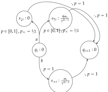
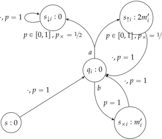
2.1 A visualization of the reduction fromDHP . . . 31

2.2 Construction from Theorem 2.3.7 . . . 40

2.3 Construction from Theorem 2.4.1 . . . 43

2.4 Construction from Theorem 2.4.2 . . . 46

2.5 The variable gadget . . . 48

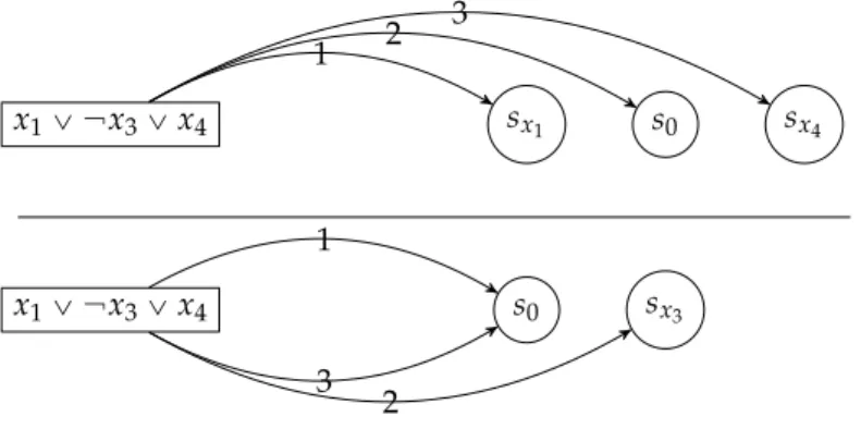
2.6 The clause gadget . . . 49

2.7 First part of the reduction in Theorem 2.5.1 . . . 54

2.8 A gadget forcingλiP t0, 1u . . . 54

2.9 (Incomplete) construction for Theorem 2.5.2 . . . 56

2.10 Main proof idea of Theorem 2.5.3 . . . 57

2.11 Illustration of the geometrical figure in proof of Theorem 2.5.3 . . . 59

3.1 Performance of the heuristic for stationary policies as a function of scenarios. . 73

3.2 Performance of the heuristic for stationary policies as a function of states . . . . 73

3.3 Performance of the heuristic for pure policies as a function of scenarios . . . 74

3.4 Performance of the heuristic for pure policies as a function of states . . . 74

3.5 Cpheuristic, evolutionaryqin dependence of state space size . . . 83

3.6 Cpevolutionary, heuristicqin dependence of state space size . . . 84

3.7 Mean time for a policy in dependence of problem size . . . 85

3.8 Evaluation of the ANTG model . . . 86

4.1 Visualization of operational, maintenance and repair phases in a single component 89 4.2 Evaluation of the composed component model with 2 components, 4 operational phases each, and one repair worker. . . 99

4.3 Evaluation of the composed component model with 3 components, 2 operational phases each, and one repair worker. . . 101

4.4 Evaluation of the composed component model with 3 components, 4 operational phases each, and one repair worker. . . 103

List of Algorithms

1 Dynamic programming algorithm for optimization of finite-horizon total

expected reward. . . 12

2 Dynamic programming algorithm for optimization of expected discounted reward . . . 13

3 Generalized policy iteration scheme . . . 13

4 Subsection 9.2.1, [Put94]: Policy iteration for the expected average criterion in MDPs . . . 14

5 Finite-horizon expected total reward optimization algorithm for stochastic games . . . 20

6 Finite-horizon expected total reward optimization algorithm for stochastic games . . . 20

7 Optimal policies for the expected average reward criterion, general scheme 21 8 Optimal policies for the expected average reward criterion, perfect informa-tion version . . . 21

9 Interval value iteration . . . 30

10 Policy iteration for expected average reward in BMDPs . . . 38

11 Exact computation ofP_ParetoandV_Pareto . . . 51

12 Percentile optimization in the simple case . . . 64

13 Local optimization heuristic for concurrent MDPs . . . 71

14 Local pure policy optimization heuristic for concurrent MDPs . . . 71

15 A heuristic forP_ParetoandV_Pareto . . . 76

16 Policy iteration to heuristically computePParetoandVPareto . . . 78

17 The SPEA2 evolutionary multiobjective optimization heuristic . . . 80

18 A simple sampling procedure to compute the minimal rate of a given phase-type distribution . . . 92

List of Tables

3.1 Performance comparison ofSPEA2and Algorithm 16 . . . 81

4.1 State and action space sizes of the generated models . . . 96

4.2 Non-dominated solution of the composed component model with 2 components, 2 operational phases each, and one repair worker. . . 97

4.3 Concurrent MDP evaluation of the composed component model with 2 compo-nents, 2 operational phases each, and one repair worker. . . 97

4.4 Concurrent MDP evaluation of the composed component model with 2 compo-nents, 4 operational phases each, and one repair worker. . . 97

4.5 Concurrent MDP evaluation of the composed component model with 3 compo-nents, 2 operational phases each, and one repair worker. . . 98

4.6 Concurrent MDP evaluation of the composed component model with 3 compo-nents, 4 operational phases each, and one repair worker. . . 98

A.1 CMDP algorithms forγ“0.9 on stochastic models . . . 110

A.2 CMDP algorithms forγ“0.9 on deterministic models . . . 112

A.3 CMDP algorithms forγ“0.999 on stochastic models . . . 114

A.4 CMDP algorithms forγ“0.999 on deterministic models . . . 116

Acknowledgments

Here I would like to mention all the people who have made this work possible. I am particularly thankful to Prof. Dr. Peter Buchholz for his comprehensive support and advice and to Prof. Dr. Holger Hermanns for a very productive month in Saarbrücken. Individual thanks goes also to my mentor who has given useful general hints on research structure and scientific procedures, Prof. Dr. Thomas Schwentick.

I also want to thank Iryna Dohndorf and Jan Kriege for the comments on the various aspects of my thesis, productive discussions, and for being patient and fun officemates.

Furthermore, I would like to thank my friends for their support during the time. Specifi-cally, I want to thank Klaus Aehlig and Moritz von Looz for the opportunities to co-operate in giving courses on games on graphs and Markov chains, respectively. I also would like to mention the various discussions on PhD-related topics, different scientific approaches and academic life in general with Carsten Burgard, Gottfried Herold, and Lucie Plaga.

Last but not least, I want to thank my family for their faith in me, and their advice and support over the whole course of my life and education until now.

Abstract

Markov decision processes model stochastic uncertainty in systems and allow one to con-struct strategies which optimize the behaviour of a system with respect to some reward function. However, the parameters for this uncertainty, that is, the probabilities inside a Markov decision model, are derived from empirical or expert knowledge and are them-selves subject to uncertainties such as measurement errors or limited expertise. This work considers second-order uncertainty models for Markov decision processes and derives theoretical and practical results.

Among other models, this work considers two main forms of uncertainty. One form is a

set of discretescenarioswith a prior probability distribution and the task to maximize the

expected reward under the given probability distribution. Another form of uncertainty is a

continuousuncertainty setof scenarios and the task to compute a policy that optimizes the

rewards in the optimistic and pessimistic cases.

The work provides two kinds of results. First, we establish complexity-theoretic hard-ness results for the considered optimization problems. Second, we design heuristics for some of the problems and evaluate them empirically. In the first class of results, we show that additional model uncertainty makes the optimization problems harder to solve, as they add an additional party with own optimization goals. In the second class of results, we show that even if the discussed problems are hard to solve in theory, we can come up with efficient heuristics that can solve them adequately well for practical applications.

1

Introduction

No decision is also a decision, and almost always the worst possible one.

— Folklore

M

choices between several alternativeactions. Simplest examples include the decision

which book to buy, what to wear, whether to repair a slight malfunction in one’s car or not etc. One challenging aspect of these choices is that the direct consequences lie in the future and cannot be foreseen from the time point of the decision. Another challenge lies in the mere fact of different possible outcomes some of which may be more preferential to the decision making agent than others.

In the domain of philosophy and economics, investigation of different aspects of choice

is known asdecision theory[Han95]. From the perspective of decision theory, to solve the

second challenge means to quantify all possible outcomes with avalue functionwhich not

only provides an order of preferences, but also numerical values which correspond to

rewardsfor each outcome. These rewards can correspond to financial benefits, but they may also represent some other, abstract units of utility. Then, given a function that maps possible actions to their respective outcomes, one can compute the optimal action that maximizes the composition of the outcome and value functions. The unpredictability of the outcomes can be modeled by means of probability theory, designing the outcome as a random variable.

In this setting, different mathematical formalisms can be considered which yield different decision models. The models may vary in the value function, the number of agents or other parameters. For example, one can think of an adversary who may make decisions on her own in order to pursue her own goals which are orthogonal to the goals of the agent whose actions one wants to optimize. A fairly popular mathematical model for

one-party decision making under stochastic uncertainty is theMarkov decision process(MDP)

formalism [Put94,Kal16] which, informally, encompasses a notion of a controlled Markov

chain with additional rewards which are paid out depending on the current state of the chain. The benefits of this formalism are twofold: First, the formalism itself allows one to model practical applications in a direct manner, and, second, efficient algorithms exist

which compute optimalpolicies, i. e., sequences of actions in dependence on the current

state.

What we want to do in this work is to consider additional notions ofmodel uncertainty

in Markov decision processes. Briefly, model uncertainty deals with the case where the parameters of the underlying mathematical model are not known exactly. In the case of decision theory, this means that the outcomes of a specific action are uncertain in the sense that even the probability distribution that defines the outcome is not precisely known. From the mathematical viewpoint, our desire is to formalize this notion of model uncertainty

and find algorithms which compute policies that arerobustagainst this uncertainty (for a

1. INTRODUCTION

1.1

Motivation

In order to motivate additional model uncertainty in Markov decision models, we provide an example.

Suppose a fictional company,Electric Till Corporation(ETC [Ste00]), is employing large

computer systems for large-scale parallel computing tasks such as deep learning, computer vision and text recognition. These computer systems consist of a number of similar

com-ponents which are bought from one supplier,Forsooth Heavy Industries(FHI) [vL13]. As

the reader may know from her own experience, computer systems may suddenly fail and generally require regular maintenance, and thus ETC needs a maintenance schedule for its computer systems which allocates (limited) maintenance personnel to the machinery, judging from typical failure times and signs of malfunctioning.

Mathematically, up to this point, this problem can be formulated as a Markov decision

process which can be solved with existing methods [Put94,Kal16]. However, in our case,

the supplier, FHI, cannot provide constant quality, be it for fabrication process features or

varying QA standards in the supply chain [WBG06]. In any case, some of the supplied

computers may fail early while some others may not require maintenance for a longer time than initially planned. This means that the behaviour, and thus the mathematical model of a single component, is subject to an uncertainty which cannot be resolved a priori by means of the model itself. Considering only the average performance also may not help here, as the costs of missing a failure may be prohibitively high compared to the costs of extra maintenance.

From this problem formulation, the ETC house expert whose task is to devise a mainte-nance schedule can pursue two different paths. On the one hand, she can consider several archetypal behaviour scenarios of the supplied hardware, such as fast failure, low main-tenance, or need for frequent maintenance yet low failure rates if maintenance is regular. The difficulty here lies in possible incomparability of the scenarios: an optimal strategy for one scenario may behave badly in the other scenario. In this setting, she can search for a maintenance policy that accounts for the relative frequency of the possible scenarios.

On the other hand, the decision maker can, from her observations, define a continuous space of possible modes of operation which also can account for possibly unseen yet probable behaviours. The main difference here is that the number of possible scenarios is infinite and the worst and best scenario are not necessarily a priori known. Here, multiple optimization goals are possible. The expert may search for the policy which is best in the pessimistic case, possibly at the cost of smaller maintenance intervals and higher load on the maintenance personnel, she also may search for a policy which is best in the optimistic case, cutting maintenance costs. Or she may search for a compromise between the two and possibly other scenarios in pursuit for a policy which behaves well in all cases without sacrificing too much.

In both cases, modeling is performed by admitting uncertainty at the level of the model; the uncertainty cannot be expressed with the means of the initial modeling formalism. In the language of Markov decision processes as base model, model uncertainty means uncertainty in the transition probabilities between states and the rewards. Especially the uncertainty in the transition probabilities offers a challenge both from the modeling and the algorithmic aspects, as the uncertainty has to be formalized in a suitable mathematical model and the policy optimization problems in these models are different from those known in the MDP literature. Knowing what algorithms are suitable and what their efficiency limits in terms of time complexity are is important, both from the theoretical point of view as well as from that of the ETC’s expert.

This thesis aims at solving these challenges from several different directions. First, we discuss mathematical formalisms that capture model uncertainty in Markov decision processes. Second, we derive complexity-theoretic results which establish lower and upper bounds for the respective optimization problems. Third, we design practically applicable 2

1.2. Structure of the thesis

algorithms for the two main problems: the multi-scenario optimization problem and the multi-objective Pareto frontier enumeration problem. Fourth, we derive a complex maintenance and repair model and its interpretations in both perspectives on uncertainty and apply our algorithms on it.

1.2

Structure of the thesis

Beside the current chapter which serves as an introduction into the topic and motivates further research, this thesis consists of two significant parts that represent two main research directions.

In the first part, Chapter2, the theoretical properties of parameter uncertainty on the

complexity of Markov decision problems are explored. We consider state-of-the-art work

and models such as those defined in [GLD00,FV97,SL73,WED94,DM10] and present own

research on the matter. The own research part concentrates around hardness results which show algorithmic limits of finite-horizon and multi-objective optimization approaches and

of related uncertainty models. This contribution is based on the conference article [Sch15],

the theoretical parts of [SBHH17] and [BS17a], and some previously unpublished remarks.

In the second part, Chapter3, we present approaches to multi-objective optimization

perspectives for uncertain Markov decision models. There, we present algorithms for vari-ous formulations of the multi-objective approach, their properties, and their experimental

evaluation. This part is based on thepracticalparts of [SBHH17] and [BS17a]. In contrast to

the previous chapter, the main results are empirical in their nature; the algorithms that are presented are judged by their performance on random data sets. The reasons for that lie in lack of efficient algorithms for the underlying problems, be it for theoretical hardness or for general lack of theoretical results.

The third part, Chapter4, contains an application of the algorithms designed in the

pre-vious chapter. While inchapter 3, the main emphasis was on performance of the individual

algorithms, here, we consider a complete path from an abstract problem formulation to the solution. In detail, we consider a model of composed components that degrade individually but can be repaired. In the model, the number of maintenance workers is limited, which limits the number of components that can be in maintenance mode simultaneously. We design uncertain Markov decision models which capture this behaviour and apply our algorithms to them.

Finally, in Chapter5, we summarize and discuss the presented results. Specifically,

we consider applications and possibilities to extend the methods to other problems and settings; furthermore, we consider possible future work on other problems in the general setting of MDPs under uncertainty.

1.2.1

Personal contribution

One of the three publications that serve as a basis for this work, namely [SBHH17], has

been completed in co-operation with other researchers. My individual contribution to this publication is the following.

• Algorithm11along with the optimality proof (Lemma2.4.5, Theorem2.4.6),

• Algorithm15,

• Algorithmic optimizations and parallelization of Algorithm16,

1. INTRODUCTION

1.3

Definitions and notation

Prior to discussing formalisms and results, we define the mathematical concepts that will be used in this thesis. The main purpose of this section is two-fold: from the mathematical point of view, we introduce the concepts that we base our results on; from a “technical” point of view, we introduce notation and identifiers. Concerning mathematical notation, we adhere to the following conventions.

• Nis the set of natural numbers, that ist1, 2, . . .u. The set of natural numbers with

zero is written asN0.

• Ris the set of real numbers. Non-negative reals are designated withRě0.

• FornPN, we abbreviate the sett1, . . . ,nubyrns.

• IfXis a set, thenPpXqis the power set ofX.

• For setsA,B, the setAZBis thedisjoint unionofAandB, a set with the properties

pAZBq zA“BandpAZBq zB“A.

• Identifiers like~v, denote vectors; if~vis ann-dimensional vector, then~vp1q, . . . ,~vpnq

are the entries of~v.

• Matrices are written in bold script, such asM. The dimensions of a matrixM are

pˆqifMhasprows andqcolumns.

• For matricesMPRpˆqwith dimensionspˆq(i. e., withprows andqcolumns), we

designate the row vectors ofMwith the notationMp1‚q, . . . ,Mpp‚q. The column

vec-tors ofMare designated byMp‚1q, . . . ,Mp‚qq; the individual entries are designated

withMpi,jqforiP rps,jP rqs.

• For square matricesMPRnˆn, the dimension ofMis denoted by dimM:“n.

• Special vectors are~1 and~0 which are column vectors of ones resp. zeros and~ei, column

basis vectors with a one in thei-th position and zeros everywhere else. When the

dimension is ambiguous, it is stated explicitly.

• The scalar product between two vectors~u,~vPRn, is designated by~u¨~vand evaluates

toř

iPrns~upiq~vpiq.

• Bystochasticmatrices and vectors we designate non-negative matricesAand vectors

~vwith unit (row) sum, that is,A~1“~1 and~v~1“1.

• Special matrices areI, the identity matrix and0, the zero matrix. Where ambiguity

may arise, a subscript will denote the dimensions of the matrix.

• The operatorbdenotes the Kronecker product, that is, for two matricesAPRmˆn,B,

the expressionAbBis ¨ ˚ ˚ ˝ Ap1, 1qB . . . Ap1,nqB .. . . .. ... Apm, 1qB . . . Apm,nqB ˛ ‹ ‹ ‚.

• The Kronecker sum, denoted by‘, defines, for two square matricesA,Bthe

expres-sionAbIdimB`IdimAbB.

1.3. Definitions and notation

• For two functions f,g:NÑN, it is fpnq “ O`gpnq˘if there existc PRě0,N PN

such that for all natural numbersnwithnąNit is _gf_pp_nnq_q ăc.

• For a setA, itsKleene closure A˚_{is the set of all finite sequences of values fromA, that is,}

finite tuplespa1,a2, . . . ,anqwithnPN0andaiPA. This especially includes the empty

tupleε. The set of all non-empty sequences overAis then given byA`“A˚_{z t}

εu.

1.3.1

Useful concepts of probability theory

As major parts of our contribution will, in one way or another, be dealing with probabilities, we briefly introduce the most important parts of probability theory we use.

Definition 1.3.1(Probabilities). LetΩ be a set, A Ă PpΩqandP:A Ñ R. The triple

pΩ,A,Pqis aprobability spaceif the following conditions are met.

• H,ΩPA.

• IfXPA, then alsoΩzXPA

• IfXiPAholds for eachXiin the sequencepXiqiPN, thenYiPNXiPA.

• PpΩq “1,PpHq “0.

• IfXi PAholds for eachXiin the sequencepXiqiPNandXiXXj“ Hfor alli,jPN,

thenPpYiPNXiq “řiPNPpXiq.

The first three conditions ensure that the set ofeventsAis aσ-algebraonΩ, and the last

two conditions definePas aprobability measureonA.

Definition 1.3.2(Conditional probability). For a probability spacepΩ,A,Pqand two events

A,B, theconditional probability of A given B, denotedP`A|B˘isPp_PpAX_BqBq.

In the sequel, we shall often adhere to the notation PrrAs, which designates the

probability of some event A, given as a logical expression. This notation is short for

Ppset of events whereAis trueqin a suitable probability space.

Definition 1.3.3 (Random variable). Arandom variable is a function X:Ω Ñ Rwhere

pΩ,A,Pq is a probability space. Often a random variable is defined by introducing a

probability density function fX: BÑRsuch thatBĎR,

ş

BfXpxqdx “1 and PrrXPMs “

PpMq “ş_MfXpxqdx.

In our discussions, we mostly skip the formal foundations and use a more simple

notation. If the probability space is obvious from the given context, we write PrrXsfor

the probability of the eventX. In some cases, to clarify that a specific probability space

pΩ,A,Pqis to be used, we use the notation PrXPAr¨s, or, if the context associates a unique

identifierxwith a probability space, Prxr¨s.

For the sake of completeness, we introduce Markov chains as the basis for generalized Markov models. The introduction of Markov chains also introduces some terminology that will be used in this thesis.

Definition 1.3.4 (Discrete-time Markov chain). Let n P N, S “ rns be a set of states,

~q “ `q1, . . . ,qn˘ P Rn a stochastic vector, andP P Rnˆn a stochastic matrix. Then the

sequencepXtpS,P,~qqqtPNof random variables onSis defined as follows.

Pr“X1pS,P,~qq “s ‰ “qs Pr”Xi`1pS,P,~qq “s|XipS,P,~qq “s1 ı “Pps1_,sq (1.1)

1. INTRODUCTION

We call such a sequence aMarkov chain on S with transition probability matrixPand initial

distribution~q.

The individual states in a Markov chain can be classified with respect to their reachability

properties. We call a stateiin a Markov chain

• absorbing, if the transition probability (or rate) to a statej‰ifrom stateiis zero,

• reachablefrom statej, if there is a path with nonzero transition probability (rate) from

statei,

• recurrent, if the probability to return toiis 1,

• transient, ifiis not recurrent.

1.4

Basic concepts of computational complexity theory

In this work, we also discuss computational complexity aspects of some problems which arise in the discussion of bounded-parameter Markov decision processes. In order to do this, we need to introduce several terms which help us to define the complexity of a problem precisely. A more thorough introduction can be found e.g., in the book of Arora

and Barak [AB09], here, we concentrate on the important results.

Complexity theory deals, in general, with the resource requirements that are imposed when a certain problem has to be solved. To establish upper and lower bounds for needed resources, we need to formally define the notion of a problem. Intuitively, we associate a

problem with deciding if an elementxof some larger setXis also an element of a subset

YĎX. For convenience, our definition imposes more structure uponX.

Definition 1.4.1(Languages and problems). LetΣbe a finite set. We then callΣanalphabet

and L Ď Σ˚ aformal languageover Σwhich may contain finitewords of the formw “

σ1σ2. . .σnsuch thatσiPΣ,iP rns,|w|:“n. Theword problemfor a given languageLis the

task to decide, for a wordwPΣ˚, ifwPL. Furthermore, we define acomputational problem

to be a languageLtogether with the word problem forL.

In the future, we use less formal language to discuss problems, however, if we talk about a problem, we implicitly assume that it can be stated as a word problem; thus,

problems are by defaultdecisionproblems. It is easy to see that this view is limited and does

not (obviously) capture usual computational tasks such as computing a matrix product. However, this perspective is still sufficiently expressive: it is possible to restate almost all known problems as decision problems by asking a sequence of binary decision questions about each bit of the output.

The central notion in computational complexity is the idea of areduction. Reductions

introduce a partial order on problems and allow one to meaningfully compare problems

with respect to their hardness and to say things like “ProblemXis not harder than problem

Y”.

Definition 1.4.2(Reduction). LetL1,L2be languages over alphabetsΣ1,Σ2. Areduction

fromL1toL2is a function f:Σ˚1 ÑΣ˚2 that satisfieswPL1ô fpwq PL2.

To define complexity, i. e., the amount of needed resources, we now face the problem of picking a machine model on which the time and space requirements are measured. It is not obvious that machine models have similar expressive power and it is even less obvious that same problems require similar space and time on different machine models. However, all

general-purpose computation models (except for possibly quantum computers [Sho94]) do

not falsify the (extended)Church-Turing thesis[vEB90].

1.4. Basic concepts of computational complexity theory

Conjecture 1.4.1(Extended Church-Turing thesis). The intuitive notion of computability is equivalent to the formal notion of computability on a Turing machine; furthermore, every deterministic machine model can be simulated on a Turing machine with at most

polynomial space and time costs, measured as function of input word length|w|.

Hence, we assume our machine model to be a random access machine (RAM) with constant costs for any arithmetic and memory access operation. The polynomial slowdown mentioned in the extended Church-Turing thesis also motivates a notion of “acceptable” or “efficient” complexity: we consider a problem to be efficiently solvable if the computational problem can be decided in polynomial time, as polynomial speedups and slowdowns are due to machine model.

Definition 1.4.3(Polynomial reductions and the classP). LetL1,L2be languages. If there

exists a reduction f fromL1toL2which can be computed in polynomial time with respect

to input size, then we writeL1ďpL2and say thatf is apolynomial reduction.

The classP(“polynomial”) is the class of all problems that can be solved in polynomial

time.

Often, however, problems are not known to be inP. Sometimes this can be proven by

showing exponential lower bounds; in some cases, there are no obvious hints. A large

number of interesting and relevant computational problems are known to belong toNP, a

superset ofPwhich is similar toPinsofar as it extendsPby non-deterministic additional

information, or advice. Intuitively,NPallows one to “guess” an advice string of at most

polynomial length with which, then, the problem can be solved in polynomial time.

Definition 1.4.4(Non-determinism and the classNP). The classNP(“non-deterministically polynomial”) is the class of all problems that can be solved with a non-deterministic RAM

in polynomial time, i.e., a languageLoverΣis inNPif and only if for eachxPLthere is a

yPΣ˚,|y| “ |x|Op1qsuch that the languageL1_{“ px,yqis inP.}

The classesPandNPare important in the sense thatPcaptures the problems which can

be solved efficiently while the classNPcaptures the problems for which a solution can be

efficientlyverified.NPobviously containsPbut there are no results that implyP“NPor

P‰NP. As previously noted, there are several important and interesting computational

problems inNPfor which no polynomial algorithm is known; furthermore, some of these

are problems which are as complex as any other problem inNP. This notion is formalized

with the help of reductions.

Definition 1.4.5(Hardness and completeness). LetLbe a language,Fa set of reductions,

andCany complexity class. If, for anyL1_{PCthere is a reduction f PFfromL}1_{toL, thenL}

is said to beC-hard under F; ifLisC-hard andLPC, thenLis said to beC-complete under F.

We restrict ourselves to the class of polynomial reductions, so, whenever we argue about,

say,NP-hardness, then we meanNP-hardness under polynomial reductions.

Many decision versions of mathematically interesting combinatorial problems areNP

-complete; among others, deciding if a graph contains a Hamiltonian path, a cycle of at most given weight, or a complete subgraph of a given size, deciding if a set of integers has a

subset whose sum has a given value, or deciding if a Boolean formula is satisfiable [Kar72].

For several problems for bounded-parameter Markov decision processes, we show that

they areNP-hard orNP-complete, too, by reducing from knownNP-hard problems. Many

years of research did not deliver a polynomial-time algorithm for any of these and many

otherNP-complete problems. This gives a reason to assume thatP‰NPimplying that

there is no algorithm that can efficiently solve all instances of anyNP-hard problem.

It is worth noting that beingNP-hard does not make a problem intractable in practice;

1. INTRODUCTION

allow for heuristics that can solve many large instances efficiently [MZ09,Hel00]; however,

a large worst-case lower bound implies at least potential problems and prohibitively slow computation of exact solutions on some large instances. In this work, we see that some of

the considered problems areNP-hard orNP-complete which is in many cases a sufficient

justification to switch to generic methods such as mathematical programming and use

mathematical programming solvers as subroutines. Such subroutines are calledoraclesin

the complexity theory world and with the help of oracles, more important problem classes can be captured.

Definition 1.4.6(Oracles andΣ₂p). LetL,L1_{be languages andCa complexity class. IfLcan}

be decided with an algorithm that calls to a subroutine that decidesL1_{, and the complexity}

of the algorithm except for the call to this subroutine is inC, thenLcan be decided with a

CL1

algorithm, aCalgorithm with an oracle for L1_.

The classNPNP, the class of all non-deterministically polynomial algorithms with an

oracle for anNP-complete problem, is also known as the classΣ₂p.

1.5

Markov decision processes and extensions

We now introduce the formalism around which this thesis is centered. Informally, a Markov decision process is a Markov chain with rewards and the possibility to select, after each transition, the transition probabilities from some pre-defined set. We briefly cover the terms and main results on Markov decision processes. A more in-depth discussion on the general

formalism can be found in [Put94,Kal16].

1.5.1

The model

Definition 1.5.1(Markov decision/reward process). Given a set ofstates S“ rns, a stochas-tic transition matrix P P Rnˆn with row sum 1, areward vector~r P Rn, and an initial

distribution vector~q PR1ˆ_ě0n with~qJ_{~1 “1, aMarkov reward processis a tuplepS,P,~r,~qq}

that defines a sequence of random variablespXiqiPNwhere PrrX1“ss “~qpsq, andXi`1for

iPNis subject to the probability distribution Pr“Xi`1“s|Xi “s1

‰

“Pps,s1_q.

For a set of statesS“ rns,actions A“ rms, a reward vector~rPRn,mstochastic transition

matricesT“

!

P1_{, . . . ,P}m)_ĂRnˆn_{, and a stochastic vector~q, aMarkov decision processis}

a tuplepS,A,T,~r,~qqwhich, for a sequence of actionspatqtPN P AN, defines sequences of

random variablespXtqandpRtqwhereX1 PSis set according to PrrX1“ss “~qpsq, and

Xi`1foriPNis subject to the probability distribution Pr

“

Xi`1“s|Xi“s1,ai

‰

“Pai_ps,s1_q;

furthermore,Rtis defined asRt“~rpXiq.

For convenience, in the Markov decision process context, we write Pr“s1 _|s,a‰

for

Pa_ps,s1_{qto designate the transition probabilities as probabilities and not just as real numbers.}

1.5.2

Alternative definitions and formalisms

In literature such as [Put94], one often defines Markov decision processes in a different

fashion. Especially, it is often assumed that a one-time reward not only depends on the state one is starting from, but also on the state after the transition and the action the controller has performed. Here, we want to argue that mathematically, our model also covers this

case. Suppose there is a functionR:SˆAˆSÑRsuch thatRps,a,s1_{qis the reward we}

get after transitioning fromstos1_{after choosing actiona.}

Then, we introduce a virtual state ˜sps,a,s1_{q for all triplesps,a,s}1_{q P SˆAˆS such}

that after selecting an action a P A, the system transitions first into the state ˜sps,a,s1_q

with the respective probability Pr“s1_|s,a‰

and then transitions intos1_{with probability 1}

1.5. Markov decision processes and extensions

(independent of the action selected in ˜sps,a,s1_{q), generating the rewardRps,a,s}1_{q. Together,}

we derive an MDP ˆ SZ ! ˜ sps,a,s1q |s,s1PS,aPA ) ,A,T,~r,~q ˙ with Paps, ˜sps,a,s1qq “Pr”s1 |s,aı Paps˜ps,a,s1_q,s1_{q “1} ~rps˜ps,a,s1qq “Rps,a,s1q ~rpsq “0 forsPS

Thus, we can efficiently eliminate a possible dependence of the rewards from the after-transition states. We note that this equivalence works by also transforming the goal function; in a way, the concept of “model equivalence” is similar to the concept of reduction we have defined above in the context of computational complexity.

We observe furthermore that our definition does not allow for states to have differing numbers of possible actions. However, this limitation can be ignored by using one action more than one time in states which have less than the maximal number of actions. In some of our proofs we will construct Markov decision processes which have different numbers of actions in different states; however, as it has been said, these MDPs can be represented with the formalism above.

1.5.3

Policies and objectives

For a Markov decision process (and its variants), several performance criteria have been proposed. We discuss some of these criteria in the context of Markov decision processes with

uncertain parameters. The most important term in this context is the term of apolicywhich

can be judged upon with the help of one of the introduced performance criteria. Informally speaking, a policy defines actions that shall be performed given a certain condition; formally,

a policy is a function f:S`_{ˆA Ñ Rthat maps (finite)historiesof states to probability}

distributions on the action space. A policy f generates, for a Markov decision process

M“ pS,A,T,~r,~qqanimmediate reward at step i

rp_ifq“ ÿ

aPA

fppH,siq,aq ¨rsi

ifsiis the current state andHPS˚is the sequence of states precedingsi.

We call a policy f

• stationaryif it depends only on the current state, i. e., if it is fppH,sq,aq “fppH1_,sq,aq

for allH,H1_PS˚_.

• deterministicif it always maps a history to a Dirac distribution, i. e.,fp¨,aq P t0, 1u,

• pureif it is stationary and deterministic,

• mixedif it is stationary, but not pure.

To clarify the nomenclature, we denote general policies with Latin identifiers, such as f;

for pure policies, we use Greek identifiers, such asπorσ. Stationary policies are denoted

with capital Greek identifiers such asΠ. Furthermore, we introduce short notation for

stationary and pure policies: we writeπpsqfor the actionawhereπp¨,s,aq “1 andΠps,aq

1. INTRODUCTION

It is easy to see that a stationary policy π induces a Markov reward process with

transition matrixPpπq_{and reward vector~r, as the transition probabilities under}

πdepend

only on the current state; this makes it mathematically easier to handle stationary policies; thus, the interest in stationary policies is justified from an “internal”, mathematical as well as from an “external”, user-centric point of view.

Having defined the notion of a policy, we now introduce tools which can measure the

performance of a given policy f in a given Markov decision process`S,A,T,~r,~q˘.

Many performance measures we define depend on one free parameter we have only

briefly mentioned, namely theinitial distribution. Different initial distributions will lead

to different distributions over the random states in the state sequence, and thus, lead to different rewards. For performance measures that depend on the initial distribution, it

is possible to aggregate all initial distributions by computing the performance measurev

for every starting state, i. e., by computing a functionvpfq_{psq “}”_vpfq_|X

1“s

ı

that maps

states to the reward measure with this starting state. This function is called avalue vector

~vpfq_PRn_{and, in many cases, finding a policy that maximizes the reward measure for one}

specific initial distribution also yields a policy that optimizes the value vector as a whole. In the following discussion, we understand under “optimization”, unless explicitly stated

otherwise, maximization of the value vector. This means that an optimal policyf adheres to

f “arg maxf~qJ~vpfq. This notion of optimality implies that there may exist more than one

policy which is optimal. Sometimes we might be interested in stationary or pure policies only; then, the existence of an optimal pure or stationary policy means the existence of a policy which is optimal in the sense defined above and, additionally, is pure or stationary.

Expected total reward A straightforward performance indicator is theexpected total reward

defined by the term

vp_Σfq“Ex » – 8 ÿ i“1 rp_ifq fi fl. (1.2)

We note that this sum does not need to converge. It does not converge if there exists at least one recurrent state with positive reward, and in general, convergence can only be guaranteed if there exist absorbing states with zero reward which are reached with probability 1. This puts a limitation on the nature of models we can consider.

Expected finite-horizon total reward To keep the mathematical properties of the expected total reward measure but to ensure also finiteness we can truncate the computation of the

expected total reward after a fixed amount of steps. This amountNPNis called ahorizon,

and the reward term turns out to be

vp_Nfq“Ex » – N ÿ i“1 rp_ifq fi fl. (1.3)

Expected average reward One useful property of the expected total reward is that this measure represents the behaviour of a policy in the infinite. For this task, we introduce two performance criteria that work independent of the nature of the underlying MDP model and converge at all times. Both of them are motivated by the expected total reward measure. As the latter does not need to be finite, it can be made finite by considering the average gain

for a time step in the long run. This measure, theexpected average rewardorexpected gain, can

be formalized by vp8fq“Ex » – lim NÑ8 1 N N ÿ i“1 rp_ifq fi fl. (1.4) 10

1.5. Markov decision processes and extensions

It can be shown [LL69] that this limit always exists for stationary policies and that there

exists an optimal stationary policy, that is, a stationary policy f “arg max_f:vpfq

8 existsv pfq 8 .

Computing the expected average reward is non-trivial for general non-stationary policies as the limit in (1.4) does not need to exist; here, we show how it can be computed for a

stationary policy f. Following [Put94], it is possible to show that the expected average

reward~vp8fqhas the following properties.

Ppfq~vp8fq“~v pfq 8

~r´~vp8fq`Ppfq~h“~h

(1.5)

The vector~his also known as thebias vectorand describes the state-dependent constant

term in the formula~hpsq `t~v8pfqpsqfor the expected gain aftertsteps, starting in states.

Expected discounted reward There are two downsides of the expected gain measure. First, it is not guaranteed that the limit in (1.4) converges for general, not necessarily

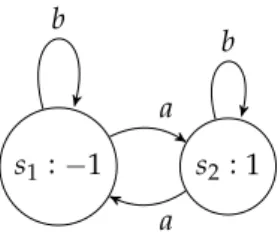
stationary policies. For example, consider a two-state MDP that is depicted in Fig.1.1. The

states offer rewards of´1 and 1, respectively, and it is possible to move to either of these

states arbitrarily. In this MDP, one can devise a policy f˘with the following behaviour: For

i PN0, the policy stays for 2itime steps ins1, gathering a total reward of´2i, and then,

f˘stays for 2itime steps ins2, gathering a total reward of 2i. Then f˘returns tos1and

stays there for 2i`1steps, gathering a total reward of´2i`1and so on. ForkPN0, the total

reward after 2p2k`1´1qsteps will be then zero, and the total reward after 2p2k`1´1q `2k`1

steps will be´2k`1. Hence, the average reward after Nsteps is then, depending on N,

somewhere between 0 and´1_{3and the limit in (1.4) does not exist.

s1:´1 s2: 1

a b

a b

Figure 1.1: A Markov decision process with a non-convergent policy

Second, the expected average measure does not differentiate betweenearlyandfuture

gains. To cope with both issues, we can introduce adiscount factorγP r0, 1qwhich describes

the “importance damping” of gains, i. e., how much less important tomorrow’s profits in comparison to those of today are.

To address these issues we introduce a different performance indicator, theexpected

discounted total reward

vpγfq“Ex » – 8 ÿ i“1 γi´1rp_ifq fi fl. (1.6)

We note that this sum always converges as there exists an upper bound on the reward (since we consider finite-state MDPs). Furthermore, one can show that for stationary policies, the

optimal policies forγÑ1 converge to optimal policies for the expected average reward

measure if the rewards are bounded [LL69] (which is always the case for finite-state and

finite-action models).

Remark. In the fully general case, a policy can depend on the complete history of a Markov decision process. However, in many applications, it may require infinite memory and thus,

1. INTRODUCTION

it seems natural to consider policies that depend only on the current state. The optimality of such policies depends largely on the kind of optimality measure; for some optimality measures such as the expected gain and expected discounted total reward, there exists

an optimal deterministic policy that only depends on the current state [Put94]; for other

measures, only policies with access to the full history are optimal.

1.5.4

Optimization of Markov decision processes

For the reward measures described above, there exist several general algorithms that find optimal policies efficiently. We briefly describe them and their properties; a more

detailed discussion can be found in [Put94]. Without limitation of generality we consider

maximization to be the main optimization direction; for minimization, symmetric arguments apply.

Dynamic programming and value iteration For total reward measures, the dynamic programming approach is straightforward as well as efficient. Intuitively, the approach consists of computing the optimal decision “in the end” where no further decisions can be made and then, by backwards induction, find optimal decisions for the preceding step under the assumption that the next step has been computed optimally. Together, this yields

Algorithm1.

Algorithm 1 Dynamic programming algorithm for optimization of finite-horizon total expected reward

functionFINITEHORIZONDYNAMICPROGRAMMING(S,A,T,~r,N)

forsPSdo~vNÐ~r

fori“N´1, . . . , 1do

forsPSdo

~vipsq Ð~rpsq `maxaPAPaps‚q~vi`1 ŹCompute the expected value

fpi,sq Ðarg maxaPAPaps‚q~vi`1

return~v1,f

This approach is also known asvalue iteration. One can observe from the structure of

the algorithm that the resulting policies depend on the state and the time step, and are

deterministic. The algorithm needs Niterations of the outer loop and in each of these

iterations,|S|inner loop iterations. Together, this makesO`

N¨ |S||A|˘time steps.

A similar approach can be used for optimizing the expected discounted reward. There, we do not have a finite amount of steps, but a convergence guarantee that stems from

Banach’s fixed point theorem [Cie07]. The modified algorithm is presented in Alg.2. The

algorithm stops when the difference between the successively computed vectorsvandv1

is smaller than εp1´γq

2γ , which implies, after Theorem 6.3.1 in [Put94], that the difference

between the resulting vectorvand the true value vector defined in (1.6) is at most ε

2for a

given precision parameterεą0. The difference between the value vector of the resulting

policyπand the value vector of an optimal policy will be at mostε.

For convenience, we provide the main argument for this statement. Banach’s fixed point

theorem states, that for a normk¨konRn and acontraction mapping L:Rn _{Ñ R}n _which

satisfieskLp~vq ´Lp~uqk ďγk~v´~ukfor someγP r0, 1q, a uniquefixed point~v˚_{exists with}

Lp~v˚_{q “~v}˚_{which can be computed by iteratively applyingLpLp. . .Lp~vqqqfor any vector~v.}

Let~v0“~vand~vn“Lp~vn´1qfornPN. Using the properties of contraction mappings and

1.5. Markov decision processes and extensions

the triangle inequality, it is possible to derive ~v˚´~v_{n`1</sub> “ Lp~v˚q ´~v<sub>n`1} ďLp~v˚q ´Lp~v<sub>n`1</sub>q `kLp~v_{n`1</sub>q ´~v<sub>n`1}k “Lp~v˚q ´Lp~v_{n`1</sub>q `kLp~v_{n`1</sub>q ´Lp~vnqk ďγ~v˚´~v<sub>n`1} `γk~v<sub>n`1}´~vnkô ~v˚´~vn`1 ď γ 1´γk~vn´~vn`1k.

This means that ifk~vn´~vn`1kďεp1´2γγq, then|~v

˚_´~v

n`1|ď ε2.

Algorithm 2Dynamic programming algorithm for optimization of expected discounted reward

functionVALUEITERATION(S,A,T,~r,γ) ~v,~v1_Ð~0PRn whileδěεp1´_2γγqdo forsPSdo ~v1_{psq Ð~rpsq `γmaxa} PAPaps‚q~v πpsq Ðarg maxaPAPaps‚q~v δÐmaxsPS ~vpsq ´~v1psq ~vÐ~v1 return~v,π

We note that the policy computed by Alg.2is pure. In fact, it can be shown that for this

performance measure, there always exists an optimal pure policy that corresponds to the

fixed point of the outer loop in Alg.2.

Policy iteration A similar result can be shown for the expected average reward measure:

in this case, too, there always exists an optimal pure policy. Furthermore, alocalityproperty

can be shown: a pure policy which cannot be optimized by changing its behaviour in one

state, i .e. a locally optimal policy, is also globally optimal. This gives rise to thepolicy

iterationapproach which is a local improvement algorithm for policies which yields optimal policies for the expected average reward and expected discounted reward measures. In the

pseudo-code description, the concrete reward measure is designated by a functionv.

Algorithm 3Generalized policy iteration scheme

functionPOLICYITERATION(S,A,T,~r,~q,v)

πÐ~0 ŹInitialize an arbitrary policy

whileπchangesdo forps,aq PSˆAdo π1 Ðπ π1psq “a ifvpπ1q_{pS,A,T,~r,~qq ąv}pπ1q_{pS,A,T,~r,~qqthen} πÐπ1 returnπ

The general scheme is depicted in Algorithm 3where v is an arbitrary optimality

criterion for pure policies. The concrete formulation of the algorithm may vary with the optimality criterion. So, for the expected average reward, the policy iteration algorithm has

1. INTRODUCTION

Algorithm 4Subsection 9.2.1, [Put94]: Policy iteration for the expected average criterion in MDPs

1: functionAVERAGEPOLICYITERATION(M“ pS,A,T,~r,~qq)

2: nÐ0, select an arbitrary decision ruleπ0

3: repeat

4: Compute~gPRn,~hPRnsuch thatPπn~g“~g,~rπn´~g`

`

Pπn´I

˘_~

h“~0

5: Choose aπn`1that satisfies

πn`1Parg max

π Pπ~g, (1.7)

keepingπn`1“πn, if possible.

6: ifπn`1“πnthen

7: Choose aπn`1that satisfies

πn`1Parg max π ´ ~rπ`Pπ~h ¯ , (1.8) keepingπn`1“πn, if possible. 8: nÐn`1 9: untilπn “πn´1 10: returnπn

Linear programming formulations As with most optimization problems, there also exists

a linear programming formulation for Markov decision problems [Man60,d’E63,Put94,

DD05]. The problem of interest here is optimizing the expected discounted reward measure.

Its main property is that the value vector~vpΠq_{for a (stationary) policyΠcan be written}

as a solution of a linear equation system~r`γPpΠq_~vpΠq _“~vpΠq_wherePpΠq_{is defined by}

PpΠq_{ps‚q “}ř

aPAΠps,aqPaps‚q. This yields a linear program which computes the optimal

value vector; this formulation has been derived by Manne [Man60].

min~1J~v

s.t.

~r`γPa~vď~v @aPA

(1.9)

The corresponding dual linear program has been introduced by d’Epenoux [d’E63,

Kal83]. maxÿ sPS ÿ aPA xs,a~rpsq s.t. ÿ aPA xs,a´γ ÿ aPA,s1_PS Paps1_,sqx s1_,a“~qpsq @sPS xs,aě0 @ps,aq PSˆA (1.10)

This formulation has several interesting properties. First, the goal function coefficients in

the primal LP can be arbitrary non-negative values and lead to the same value of~v. Second,

the optimal policy can be read from the solution by looking at the rows of the primal LP that are tight; if the constraint

~rpsq `γPaps‚q~vď~vpsq (1.11)

is tight, that is, if it is~rpsq `γPaps‚q~v“~vpsq, then the optimal policy selects the actionain

states. Third, by complementary slackness, the variablesxs,ain the dual formulation that

1.5. Markov decision processes and extensions

correspond to the rows in (1.9) are nonzero if and only if the constraint (1.11) is tight. This

means that the variablexs,ain the dual formulation can be used as “decision variable” that

is nonzero if and only if the optimal policy selects the actionain states. However, these

are not decision variables in the sense of combinatorial optimization, as they do not have to be integral. The most common interpretation for these variables is that they describe “discounted visitation frequencies” of states that contribute to the cumulative reward.

Nevertheless, there are ways to derive integral variables from the variables of the dual

formulation [DD05]. A simple way to do so is by introducing additional integer variables

ds,aP t0, 1uwith the constraintsds,a“1ôxs,aą0; alternatively, an equivalent constraint is

ds,a“ ř xs,a

a1PAxs,a1. In general, this constraint cannot be written as a linear inequality; however,

here we know thatxs,ahas an upper bound of _1´1_γas the rewards from a statesare bounded

by ~_1´rpsq_γ. This allows us to impose the constraintds,a¨_1´1_γ ěxs,afor allps,aq PSˆAand

ř

aPAds,a “ 1 for alls P S. Together, we can derive the following mixed-integer linear

program. maxÿ sPS ÿ aPA xs,a~rpsq s.t. ÿ aPA xs,a´γ ÿ aPA,s1_PS Paps1_,sqx s1_,a“~qpsq @sPS ÿ aPA ds,a“1 @sPS ds,aě p1´γqxs,a @ps,aq PSˆA xs,a ě0 @ps,aq PSˆA ds,aP t0, 1u @ps,aq PSˆA (1.12)

From the complexity-theoretic point of view, it is easy to see that almost all MDP problems can be solved in polynomial time. As we extend the MDP formalism, an important question is if this property can be kept.

1.5.5

Continuous-time processes and uniformization

A large body of research deals with the question what happens if the transition times in a Markovian decision process are not equal but also distributed according to a memoryless distribution which depends on the state (and sometimes the selected action). Following this research question, one arrives at the continuous-time MDP model. Its main characteristic is that the evolution of the underlying system is defined by a system of (linear) differential equations. In the next paragraphs, we give a brief overview of the formalism and describe a method to analyse some aspects of continuous-time MDPs with algorithms for discrete-time Markov decision processes.

Continuous-time Markov chains Similarly to a discrete-time Markov chain, one can de-fine continuous-time Markov chains where the transition times are governed by exponential distributions. Concretely a continuous-time Markov chain can be represented by a

stochas-tic vector~q0 P R1ˆn and a rate matrix Q P Rnˆn for which the properties Q~1 “~0 and

Qpi,jq ě0 for alli‰jwithi,jP rnshold.

The evolution of a continuous-time Markov chain can be described as follows. The

system stays in a statesPSfor a time interval which is negative exponentially distributed

with rateQps,sqand then performs a transition to another states1_{with probability} Qps,s1q

1. INTRODUCTION

A global representation of this dynamics is the differential equation [Kol31]

d~pptq

dt “~pptqQ

~pp0q “~q

(1.13)

where~pptqis the probability distribution of the Markov chain being in a given state at time

t. The solution to this equation is~pptq “~qexppQtqwhere the matrix exponential exppMqis

defined by the infinite sum

exppMq “ 8 ÿ i“0 Mi i! . (1.14)

Continuous-time Markov decision processes With a continuous-time Markov chain for-malism, we arrive at a formalism for continuous-time MDPs.

Definition 1.5.2. Given a Markov decision process`S,A,T,~r,~q˘and a vector~βPRnwith

~_{β ą 0, acontinuous-time Markov decision process(CTMDP) is a tuple}´_S,A,T,~r,~q,~_β¯_{. A}

CTMDP defines not only a sequence of states as described in Def.1.5.1, but also a sequence

ofsojourn timespYtqtPNwhereYtis exponentially distributed with parameter~βpXtq.

Together, they define a family of random variablespYxqxPRě0 withYx“Xtif

ř

t1_ătY_t1 ă

xandř

t1_ďtY_t1 ěx.

This definition expands the MDP formalism by the notion of transition times. It is easy to see that the system retains its Markovian property: The sojourn time does not depend on the starting point of the observation. Mathematically speaking, for an exponentially

distributed transition timeYit is PrrYěxs “Pr“YěT`x|YěT‰for allxě0,Tě0.

The finite-horizon total reward for a time horizonTin this model is formalized by the

integral expression

żT

0

~rpYxqdx (1.15)

which allows us to derive the expected average total reward lim TÑ8 1 T żT 0 ~rpYxqdx (1.16)

and the expected discounted total reward with adiscount rateαą0

ż8

0

expp´αxq~rpYxqdx. (1.17)

Uniformization Analysing continuous-time MDPs means, in the most general case,

ana-lyzing a continuous-time system that is governed by a set of differential equations [Put94];

especially the finite-horizon case is less simple to analyse as the number of transitions in a finite time interval can be unbounded. We note here that even for the finite-horizon case

optimal policies can be computed [BDS17b], but as our main results consider “stationary”

optimality criteria such as the expected discounted total reward and the expected average reward, we provide a tool that enables to analyse continuous-time MDPs with discrete-time

methods with respect to these criteria [Put94].

The uniformization technique amounts to two steps: First, the stochastic process is transformed into a process with uniform sojourn time distribution in all states. Second, as the sojourn times are distributed equally, the expected rewards in each state are computed 16

1.6. Stochastic games

and only the transition probabilities with these new rewards are considered, which allows one to use discrete-time methods.

Informally, the first step of the uniformization procedure transforms the continuous-time process into another continuous-time process where the transition events occur with equal frequency in each state. For this, the transition probabilities are modified in order to keep the total sojourn time.

Concretely, to transform a continuous-time MDPpS,A,T,~r,~q,~βqinto a discrete-time

MDP pS,A,Tu,~ru,~qq, the following steps have to be made. First, theuniformization rate

β˚ ěmaxiPS~βpiqis chosen. Then, a CTMDPpS,A,Tu,~r,~q,β˚~1qis computed by defining

Tu“ ! P1 u, . . . ,Pum ) with Puaps,s1q “ $ ’ & ’ % 1´p1´P a_ps,sqq~_βpsq β˚ s“s 1 Paps,s1_q~_βpsq β˚ s‰s 1 (1.18)

Then, the rewards have to be adjusted. For the expected average total reward, we set

~rupsq “

~rpsq

β˚ . (1.19)

For the expected discounted total reward, we set

~rupsq “

~rpsq

β˚`α (1.20)

and introduce the discount factorγ“ β

˚

β˚`α. It can be shown that a stationary policy will

yield for theseuniformizedprocesses the same optimality values as for the original CTMDPs,

which allows us to use discrete-time analysis methods in order to find optimal policies for

the expected average and expected discounted reward criteria [Ser79,Put94].

1.6

Stochastic games

It is easy to see that we can consider a Markov decision process as a game where the controller can choose actions and the randomness chooses following states. This view can be generalized in a natural way to more parties. For us, of special interest is the two-player

case, where two parties can control the system, thecontroller(CON) andNature(NAT).

In the literature [Sha53,FV97], these processes are known asstochastic games. Informally,

in a stochastic game, CONand NATchoose from two pools of availableactions; the action

pair combined with the current state defines a probability distribution on the next state and a reward value.

Definition 1.6.1(Stochastic game). For a set of statesS“ rnsand two action setsAC,AN, astochastic gameis a tuplepS,AC,AN,P,~rC,~rN,~qqwhereP:SˆACˆANÑSÑRis, for

every tripleps,aC,aNq, a probability distribution on states,~qPRnis a stochastic vector, and

~rN,~rCPRnarereward vectors.

The semantics of a stochastic game is straightforward: At each discrete time stept,tPN,

the formal system is in a states PS. CONchooses an actionaCfrom thecontroller action

set ACand NATchooses an actionaNfrom thenature action set AN. Then, animmediate

rewardprC,rNq “

`

~rCpsq,~rNpsq

˘

is being paid off; CONgains~rCpsqreward units and NAT

gains~rNpsqreward units. Then, the system performs a transition to a state s1 P Swith

probabilityPps,aC,aNqps1q. Formally, a stochastic game together with a sequence of action

1. INTRODUCTION PrrX1“ss “~qpsqand Pr “ Xi`1“s1|Xi“s,aC,i“aC,aN,i“aN ‰ “ Pps,aC,aNqps1q. The

sequencepXiqiPNalso defines a sequence of random reward pairsprC,i,rN,iqiPNwithrC,i“

~rCpXiqandrN,i“~rNpXiq.

It is important to distinguish an important subclass of stochastic games with special

semantics: In aperfect information stochastic game, NAT and CON perform actions by

alternating their moves, that is, both players can observe the results of each other’s action

before making the next move. This is modeled by separating the state setSinto two disjoint

subsets, thecontroller set SCONand thenature set SNATwithS“SCONZSNAT; the semantics

is such thatPps,aC,aNq “Pps,aC,a1NqforsPSCONand allaN,a1_N PAN, and, symmetrically,

Pps,aC,aNq “Pps,a1_C,aNqforsPSNATand allaC,a1CPAC.

For a stochastic game, the most interesting question is if there is a policy for CONwhich

maximizes her overall performance measure while NATtries to maximize her own overall

performance measure. The answer to this question mainly depends on the structure of~rN

and~rCand the chosen optimality criteria. For the latter, we assume that the optimality

criteria are the same for both players (and have the same optimization direction), that is, if

prC,iqiPNandprN,iqiPNare the payoff sequences for each of the players, then the optimality

criterion can be described by a single functionv:RNÑRsuch that the goal functionvC

for CONisvpprC,iqiPNqand the goal functionvNfor NATisvpprN,iqiPNq. For the former, we

consider two cases that are most important to us, namely, thecooperativeand thecompetitive

cases.

The cooperative case~rCě~0,~rN “~rC

The competitive case~rCě~0,~rN“ ´~rC

It is easy to see that in the cooperative case, there is no conflict in the goals of CONand

NAT. This means that finding the optimal policy for the cooperative case can be performed

with the methods known from Markov decision process optimization. In fact, replacing both players with one party leaves us with a Markov decision process (under the assumption that the optimality criteria for both players are the same).

Optimal policies for stochastic games Previously, we have established that cooperative stochastic games are equivalent to Markov decision processes. Here, we consider competi-tive stochastic games and briefly outline the most important algorithms that find optimal

policies. A more complete discussion is available in the original work of Shapley [Sha53]

and in the textbook of Filar and Vrieze [FV97]; the facts that are mentioned here are reduced

to the ones we need in the rest of our work.

Apolicy pairin a stochastic game is a pair of functions fC:S`ˆACÑ r0, 1s,fN:S`ˆ

AN Ñ r0, 1sthat define probability distributions over actions in dependence of previous

visited states and random reward sequencesprp_Cf_,C_i,fNqqiPN,prpNf,Ci,fNqqiPN. In analogy to the

MDP case, we assume that there exists an optimality criterion that yields real values

vpfC,fNq

C ,v

pfC,fNq

N which describe the goal functions of the two players for each policy. We call

a policy pairpf˚

C,fN˚qoptimal, if the following conditions are met.

• vpf ˚ C,fN˚q C ěv pfC,fN˚q C for each fC:S`ˆACÑ r0, 1s • vpf ˚ C,fN˚q N ěv pf˚ C,fNq N for eachfN :S`ˆANÑ r0, 1s

Now we consider different optimality criteria and the corresponding algorithms. The optimality criteria are similar to those defined for Markov decision processes.

1.6. Stochastic games

The finite horizon total expected reward criterion For a finite horizonNPN, the finite horizon total expected reward criterion for stochastic games is defined by

vpfC,fNq C,N “Ex » – N ÿ i“1 rpfC,fNq C,i fi fl vpfC,fNq N,N “Ex » – N ÿ i“1 rpfC,fNq N,i fi fl (1.21)

In the sequel, we only give the optimality criterion for CON, as the criterion for NATis

defined symmetrically.

To compute an optimal policy pair for the finite horizon total expected reward criterion,

we perform a similar procedure to the one in Algorithm1, adjusted for the two-player case.

In fact, the most challenging task here is to compute a decision rule that is optimal, as we move from a simple maximization problem to a max-min problem.

In order to derive a solution, we consider simple one-step two-player games first.

Definition 1.6.2(One-step game). For finite action spacesAC “ rmCs,AN “ rmNs, a

one-step gameis defined by a matrixCPRmCˆmN_{with the following semantics: If CONchooses}

actionaCPACand NATchooses actionaNPAN, then the payoff for CONisCpaC,aNqand

the payoff for NATis´CpaC,aNq.

An optimal policy for a one-step game can then be computed by solving the following linear program. maxv s.t. vď ÿ a_CPA_C ~xpaCqCpaC,aNq @aNPAN ÿ a_CPA_C ~xpaCq “1 ~xě~0 (1.22)

The result of this optimization problem is thevalueof thematrix gamedefined byC; the

optimal policy is given implicitly in the decision vector~x. We observe that~x does not

necessarily have to define a Dirac distribution; hence, for general stochastic games policies may not necessarily be deterministic.

This result can be used in order to derive optimal policies for stochastic games with

arbitrary finite horizons. In detail, knowing the optimal policy for future steps in stepn

and the corresponding valuevps1_{,n`1qof all statess</sub>1<sub>PSin then`1st step, the choice for}

players CONand NATin statescorresponds exactly to a one-step game with matrixCn,s

which is defined byCn,spaC,aNq “řs1_PSPps,aC,aN,s1qvps1,i`1q.

For perfect information s