Sonderforschungsbereich/Transregio 15 www.sfbtr15.de
Universität Mannheim Freie Universität Berlin Humboldt-Universität zu Berlin Ludwig-Maximilians-Universität München Rheinische Friedrich-Wilhelms-Universität Bonn Zentrum für Europäische Wirtschaftsforschung Mannheim
Speaker: Prof. Dr. Urs Schweizer. Department of Economics University of Bonn D-53113 Bonn,
*University of Bonn **Humboldt-University Berlin
January 2010
Financial support from the Deutsche Forschungsgemeinschaft through SFB/TR 15 is gratefully acknowledged.
Discussion Paper No. 303
Optimal Procurement Contracts
with Pre–Project Planning
Daniel Krähmer* Roland Strausz**
Optimal Procurement Contracts with Pre–Project
Planning
Daniel Kr¨ahmer
∗and Roland Strausz
†January 18, 2010
Abstract
The paper studies procurement contracts with pre–project investigations in the pres-ence of adverse selection and moral hazard. To model the procurer’s problem, we extend a standard sequential screening model to endogenous information acquisition with moral hazard. The optimal contract displays systematic distortions in information acquisition. Due to a rent effect, adverse selection induces too much information acquisition to prevent cost overruns and too little information acquisition to prevent false project cancelations. Moral hazard mitigates the distortions related to cost overruns yet exacerbates those related to false negatives. The optimal mechanism is a menu of option contracts that achieves the dual goal of providing incentives for information acquisition and truthful in-formation revelation.
Keywords: Information acquisition, procurement, dynamic mechanism design JEL codes: D82, H57
∗University Bonn, Department of Economics and Hausdorff-Center for Mathematics, Adenauer Allee 24-42,
D-53113 Bonn (Germany), [email protected].
†Humboldt-Universit¨at zu Berlin, Institute for Microeconomic Theory, Spandauer Str. 1, D-10178 Berlin
(Germany), [email protected]. We thank the editor, two anonymous referees, Pascal Courty, Peter Es¨o, Regis Renault and seminar participants in Barcelona, Berlin, Bonn, Cambridge, Heidelberg, Mannheim, Michi-gan, Munich, Rotterdam. Both authors gratefully acknowledge financial support by the DFG (German Science Foundation) under SFB/TR-15. Roland Strausz further acknowledges support under DFG–grant STR991/2-2.
1
Introduction
Practitioners in managing procurement projects stress the importance of pre–project planning. Based on a number of case studies, Gibson and Hamilton (1994) conclude that “there does exist a positive, quantifiable relationship between effort expended during the pre-project planning phase and the ultimate success of a project.”1 The goal of pre–project investigations is to obtain
more accurate cost estimates, which allow the procurer to decide more carefully about whether to implement the project. In other words, pre–project planning is a process of information
ac-quisition before the final implementation decision is taken.2 The project management literature
not only stresses the importance of effective pre–project planning but also warns procurers to keep as much control over this process as possible. For instance, Gibson et al. (2006, p.41) write in their empirical appraisal that procurers frequently “decide to delegate the pre-project planning process entirely to contractors, often with disastrous results”. Given the importance of pre–project planning and these observed “disastrous results” from delegation, we develop and analyze an economic model of pre–project planning to enhance our understanding of this process.
Our starting point is the observation that the reported “disastrous results” from delegation point to conflicting interests and incentive problems. Due to the contractor’s superior exper-tise, we can identify three sources of incentive problems in pre–project investigations. First, the contractor is already in a better position to estimate the project’s cost from the very out-set. Hence, the procurer–contractor relationship typically exhibits ex ante adverse selection. Second, the contractor, as the expert, is often in the better position to evaluate the additional information which the pre–project investigation reveals. Hence, pre–project investigations lead to additional adverse selection at an interim stage. Third, the amount of information that results from pre–investigations will largely depend on the contractor’s own actions such as his advice and expertise on how to perform the investigations. Hence, pre–project investigations also involve a moral hazard problem.
1
See also, e.g., Turner (1993), Gibson et al. (2006), K¨ahk¨onen (1999) and Dahlin, Bjelm, and Svensson (1999).
2
Gibson et. al. (1995) define pre–project planning “as the process of developing sufficient strategic informa-tion for owners to address risk and decide whether to commit resources to maximize the change for a successful capital facility project”.
The presence of these three different types of incentive problems leads us to view the pro-curement problem as a dynamic mechanism design problem. To capture adverse selection, we adopt a sequential screening approach as in Courty and Li (2000) and Es¨o and Szentes (2007b). To capture moral hazard, we allow for unobservable interim information acquisition by the agent. Our results are as follows. First, we derive as a benchmark the first–best solution with-out any incentive problems. In this case, the principal uses pre–investigations to mitigate one of two implementation errors: If the initial information about the project is favorable and indi-cates a positive social value, then the principal uses pre–investigation to prevent cost overruns. For this case, we say that information acquisition prevents false positives (or type I errors). In contrast, if the initial cost information is unfavorable, then she uses pre–investigations to correct for a possibly false cancelation of the project. Information acquisition then prevents false negatives (or type II errors).
Second, we characterize the optimal contract when information acquisition is still observable but there are adverse selection problems. In this case, the principal implements the optimal contract by a menu of contracts that offers a fixed price contract and a range of option con-tracts. The fixed price contract obliges the contractor to carry out the project in all cost circumstances for a fixed price. The option contract gives the contractor the right to first conduct a pre–investigation and then decide whether to complete the project for an exercise price or, alternatively, quit the project. As we will argue in Section 7, option contracts feature prominently in a range of real world contractual relations and support our analysis.
Third, we treat the case with unobservable information acquisition and characterize the conditions under which the implied moral hazard problem causes additional agency costs. In particular, we find that additional agency costs do not arise when the contractor’s additional information is uncorrelated with his initial information. In general, however, moral hazard does cause additional agency costs. We demonstrate that, in this case, the principal has to adapt the contract in ways that leads to bunching and less information acquisition.
Finally, the comparison of the optimal contract under the three different contracting en-vironments allows us to characterize the systematic distortions in information acquisition and attribute them to the different incentive problems. We first demonstrate that the adverse selec-tion problem leads to too much informaselec-tion acquisiselec-tion to prevent false positives (type I errors)
and too little information acquisition to prevent false negatives (type II errors). Moreover, we show that the moral hazard problem unambiguously exacerbates distortions with respect to type II errors and mitigates distortions with respect to type I errors. As a result, the welfare effects of the additional moral hazard problem are ambiguous. While the principal always loses from additional agency costs, the agent’s utility and, in fact, total welfare may go up in the presence of a moral hazard problem. In this case, the moral hazard problem mitigates some of the inefficiencies from adverse selection.
Our paper contributes to the growing literature on optimal dynamic mechanism design. This literature studies optimal contract design in environments in which information is privately
revealed to the agents over time.3 A recent paper by Pavan et al. (2008) provides a general
framework that encompasses earlier contributions on dynamic price discrimination (e.g., Baron and Besanko (1984), Laffont and Tirole (1990, 1996), Battaglini (2005)), or on sequential screening (e.g. Courty and Li (2000), Dai et al. (2006), Es¨o and Szentes (2007a, b)). Our contribution to this literature is to extend the analysis to endogenous information acquisition with moral hazard.
Our basic setup is most similar to the sequential screening model by Courty and Li (2000) who study monopolistic price discrimination when consumers are uncertain about their
subse-quent demand but obtain additional information before actual consumption.4 Similar to Courty
and Li (2000), we impose a first order stochastic dominance ranking condition on the family of
the conditional cost distributions conditional on the initial signal.5 A well–known,
fundamen-tal problem is that, unlike in static problems, incentive compatibility in sequential screening problem cannot be characterized in terms of monotonicity of the allocation rule. Courty and Li (2000) therefore first uncover necessary conditions for incentive compatibility from “local” constraints and then use the stochastic dominance ranking to verify implementability. We give a new proof for the validity of this approach by showing that for deterministic contracts, incen-tive compatibility can actually be characterized in terms of monotonicity. This property then allows us to treat the case when information acquisition is endogenous. The optimal contract
3
A number of papers deals with the design of efficient mechanisms in dynamic environments. See, e.g., Athey and Segal (2007a, 2007b), Bergemann and V¨alim¨aki (2008).
4
Es¨o and Szentes (2007a) extends Courty and Li (2000) to a multi–agent setting.
5
derived by Courty and Li (2000) also displays a menu of option contracts. Thus, our analysis makes clear that option contracts are a robust feature of optimal sequential screening contracts also if information acquisition is endogenous and, possibly, involves moral hazard problems. In fact, such options not only work to screen consumers, but serve the additional purpose of inducing information acquisition.
Closely related is also the model by Es¨o and Szentes (2007b), where the principal can acquire costly, additional information which only the agent can interpret. We differ from Es¨o and Szentes (2007b) in at least three respects: first, in our model it is the agent who acquires additional information. More importantly, while Es¨o and Szentes (2007b) restrict attention to observable information acquisition, we also analyze the natural case when it is unobservable. This leads to a moral hazard problem that changes the analysis fundamentally. A final difference is that we characterize and give an intuitive explanation for the distortions
in information acquisition that are implied by adverse selection and moral hazard.6
Our work is also related to the literature on information acquisition in principal–agent problems (e.g., Lewis and Sappington 1997, Cremer et al. 1998, Kessler 1998, Szalay 2009). The key difference is that this literature studies the incentives of an agent to acquire private informationbefore he accepts or rejects the contract. Therefore, there is only a single screening stage.
The rest of the paper is organized as follows. The next section introduces the model. Section 3 discusses the first–best benchmark. In Section 4, we present the principal’s problem. In Section 5, we solve the principal’s problem when information acquisition is publicly observable and derive the distortions implied by optimal contracting. In Section 6, we treat the case with unobservable information acquisition. In Section 7, we discuss empirical implications of the theory. Section 8 concludes.
2
Model
A principal seeks to procure one unit of a good from an agent. The principal’s valuation for
the good is v >0. There are two periods. In period 1, contracting takes place, and in period
6
See also Hoffmann and Inderst (2009), who study the distortions in information acquisition due to adverse selection only.
2, the agent produces the good. Before contracting, the agent privately observes a noisy signal
about true costs. Let the noisy signal be given by the random variable ˜γ and let true costs be
given by the random variable ˜c. The agent privately observes the realization γ of ˜γ, and it is
common knowledge that ˜γ is distributed with distribution function F and density f =F′ on
the support Γ = [0,γ¯]. We assume that f is strictly positive and differentiable on Γ and that the hazard rate h(γ)≡F(γ)/f(γ) is non–decreasing in γ.
True costs are equal to the signal plus a random shock ˜s: ˜c = ˜γ + ˜s. The cost shock
has support R and has zero conditional mean so that ˜γ is an unbiased estimate of costs:
E[˜c|γ] = γ+E[˜s|γ] = γ.7 In general, the distribution of ˜c conditional on γ is given by G(·|γ)
with the conditional density g(·|γ).8 We assume that the family {G(·|γ)}
γ is ranked in terms
of first order stochastic dominance. That is,G(·|γ) first order stochastically dominates G(·|γ′)
whenever γ > γ′. A lowγ therefore indicates a low actual cost c.
A specific version of our model is theindependent case, where the distribution of the shock
is independent of γ. Formally,
G(c|γ) = ˆG(c−γ), (1)
where ˆG is the distribution function of the shock s. For expositional clarity, we focus on the independent case whenever this does not affect results qualitatively. The independent case is natural when the cost shock is independent of the agent’s average efficiency characteristics such as expertise, experience, or internal organization. A specific example is an infrastructure project and the uncertainty pertaining to soil conditions or ground water levels. The independent case automatically satisfies the first order stochastic dominance ranking of{G(·|γ)}γ.
After the contract has been signed and before production takes place, the agent can, at a cost k > 0, perfectly observe s and therefore learn the actual cost c. While the value of k is common knowledge, the principal cannot observe which information the agent receives. Hence, from the principal’s perspective, there is adverse selection at the contracting as well as after the
7
The additive specification is without loss of generality because the shock can always be defined as the difference between true and expected costs. The assumption that the support of the shock, and thus of true costs, isRis for convenience only and standard in the literature.
8
Throughout we assume, for technical reasons, that all partial derivatives of h, G, and g exist and are bounded.
information acquisition stage. We will consider both observable and unobservable information acquisition. In the latter case, there is an additional moral hazard problem at the information acquisition stage. Finally, we assume that at the contracting stage the principal makes a take–it or leave–it offer. If the agent rejects, he gets a type–independent outside option of zero.
3
First–best
As a benchmark, we first consider a first–best world, in which information acquisition and all available information is publicly observable. In a first best world, the two crucial questions
are for which cost estimates γ the agent should acquire additional information and when to
execute the public project. Hence, a first–best contract specifies, first, for each agent type γ a probabilityαF B(γ) with which the agent acquires information. Second, it specifies a probability
qF B(γ, c) with which the project is executed by an agent who has acquired information and
whose true costs turn out to be c. Finally, the contract determines a probability ¯qF B(γ) with which an agent who has not acquired information executes the project.
The answer to the question when to execute the project is straightforward. Depending on
whether true or expected costs are above or below the valuationv, the production probabilities
in the first best are either zero or one. Formally,
qF B(γ, c) = 1 if v ≥c 0 if v < c , q¯ F B(γ) = 1 if v ≥γ 0 if v < γ . (2)
With these efficient implementation decisions, we can determine the first–best information acquisition levels and understand how, in a first best world, information is used.
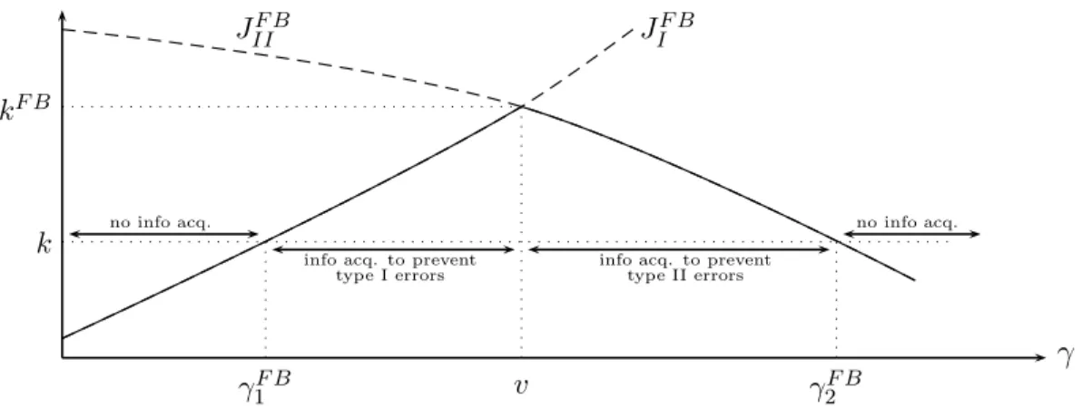
Depending on the implementation decision in the absence of additional information, the acquisition of information plays one of two roles. First, if the decision without information
acquisition is to implement the project, then the procurer commits atype I error if cturns out
to be larger thanv. In this case, a loss v−c is realized. Information acquisition prevents this error. Formally, the (gross) expected value of information to prevent type I errors is
JIF B(γ)≡
Z ∞ v
Second, if the decision without information acquisition is to cancel the project, then the
procurer makes a type II error if c turns out to be smaller than v. Information acquisition
prevents this error, and thus the (gross) expected value of information to prevent type II errors is
JIIF B(γ)≡
Z v
−∞
(v−c)dG(c|γ). (4)
According to the first–best implementation decision (2), the procurer optimally implements
the project without additional information whenever γ ≤ v. Hence, the first–best value of
informationis JF B(γ)≡ JF B I (γ) if γ ∈[0, v] JF B II (γ) if γ∈(v,γ¯]. (5)
Because γ is an unbiased estimate of actual costs, JF B is continuous at γ = v.9 Moreover,
the first order stochastic dominance ranking of{G(·|γ)}γ implies that JF B is increasing in the range γ ∈ [0, v] and decreasing in the range γ ∈ (v,γ¯]. Hence, JF B is single peaked with its
maximum at γ =v. Let kF B ≡JF B(v) denote this maximum. Figure 1 illustrates the typical
shape of the curve JF B.
Information acquisition is efficient for all γ with JF B(γ) ≥ k. Because JF B attains a
maximum at γ =v, information acquisition is never efficient if k ≥ kF B. Whenever k < kF B, single–peakedness of JF B implies that there exist exactly two cut–offs γF B
1 < v < γ2F B, which
satisfy
JIF B(γ1F B) = k, JIIF B(γ2F B) =k. (6)
Thus information acquisition is efficient if γ ∈ [γF B
1 , γF B2 ]. The next proposition summarizes
these results, and Figure 1 illustrates.
Proposition 1 The first–best implementation probabilities are given by (2). Moreover, it holds:
(i) If k < kF B, the first–best information acquisition probabilities are
αF B(γ) = 1 if γ ∈[γF B 1 , γ2F B] 0 if γ 6∈[γF B 1 , γ2F B] . (7)
(ii) If k ≥kF B, the first–best information acquisition probability is αF B(γ) = 0 for all γ.
9 Note: R∞ v (c−v)dG(c|γ) = Rv −∞(v−c)dG(c|γ)⇔ R∞ −∞(c−v)dG(c|γ) = 0⇔γ−v= 0.
γ JF B I JF B II kF B v k γF B 1 γ2F B
info acq. to prevent type I errors
info acq. to prevent type II errors
no info acq. no info acq.
Figure 1: First–best information acquisition
4
The principal’s problem
We now return to the original problem with asymmetric information and look for the contract that maximizes the principal’s payoff. A contract specifies a transfer and the probability with which the agent has to produce the good in period 2, which, in principle, can be made contingent on arbitrary forms of communication between the parties. A crucial step to reduce the number of possible contracts is to apply the revelation principle for multistage games (Myerson 1986), which asserts that the optimal contract can be found in the class of direct, incentive compatible mechanisms.
A direct mechanism has the following structure: First, it requires the agent to submit a
report ˆγ ∈ Γ in period 1. Subsequently, the mechanism gives a contingent, possibly
proba-bilistic, recommendation to the agent whether or not to acquire information. Let α(ˆγ) be the
probability with which the contract recommends information acquisition. For the case that information acquisition is not recommended, the contract specifies the transfers ¯t(ˆγ) from the principal to the agent and the probability of production ¯q(ˆγ). When information acquisition
is recommended, the agent is required to submit a second report ˆc ∈ R in period 2,
result-ing in transfers t(ˆγ,ˆc) and the probability of production q(ˆγ,cˆ). Thus, a direct contract is a combination (α,¯t,q, t, q¯ ).
A direct contract is incentive compatible when it induces truthtelling and obedience.
Truth-telling means that, on the equilibrium path, the agent has an incentive to report his new information truthfully. Obedience means that, on the equilibrium path, the contract must
give the agent an incentive to follow the contract’s recommendation whether or not to acquire information.
Formally, let ΓI ={γ ∈Γ|α(γ)>0}denote the set of agent types that acquire information with a strictly positive probability. Then truthtelling in period 2 requires for allγ ∈ΓI that
t(γ, c)−cq(γ, c)≥t(γ,cˆ)−cq(γ,cˆ) ∀c,cˆ∈R. (AS2) To state the first period truthtelling constraints, let U(γ) denote the utility of agent type γ
if he reports truthfully and obeys the contract’s recommendation:
U(γ)≡α(γ) Z ∞ −∞ t(γ, c)−cq(γ, c)dG(c|γ)−k + (1−α(γ))[¯t(γ)−γq¯(γ)]. (8)
Incentive compatibility means that the agent cannot attain a higher utility than U(γ) by
adopting an untruthful reporting and/or disobedient information acquisition strategy. Notice that whatever the agent does in period 1, if he is required to submit a report in period 2,
the second period constraints (AS2) guarantee that he reports truthfully in period 2.10 Hence,
even though the revelation principle does not require it, our setup yields truthtelling also off
the equilibrium path.11 With this in mind, we now consider all the deviations which incentive
compatibility is meant to prevent and classify them in three different groups.
First, an agent type γ must not gain by reporting some type ˆγ and, subsequently, obey the
contract’s information acquisition recommendation:
U(γ)≥α(ˆγ) Z ∞ −∞ t(ˆγ, c)−cq(ˆγ, c)dG(c|γ)−k +(1−α(ˆγ))[¯t(ˆγ)−γq¯(ˆγ)] ∀γ,γˆ ∈Γ. (AS1)
Moreover, an agent typeγ must not gain by reporting ˆγ and then disobeying when the contract
requires him to acquire information:
U(γ)≥α(ˆγ)[t(ˆγ, γ)−γq(ˆγ, γ)] + (1−α(ˆγ))[¯t(ˆγ)−γq¯(ˆγ)] ∀γ,γˆ∈Γ. (MH)
Finally, an agent type must not gain by disobeying when the contract requires him not to acquire information. However, this cannot be optimal for any agent type, because when no
10
E.g., expected utility of a typeγ, who is ignorant of his actual costsc and reports some costs ˆc, ist(γ,ˆc)−
q(γ,ˆc)R
cdG(c|γ) =t(γ,cˆ)−q(γ,ˆc)γ. According to (AS2) his payoff is maximized for a report ˆc=γ.
11
This would be different if the support of final costs c depended on the first period information γ. See Kr¨ahmer and Strausz (2008) for a discussion of the case when the supports of final costs do not overlap.
information acquisition is recommended, transfers and implementation probabilities do not
condition on the additional cost informationc so that the value of information for the agent is
zero. Thus, the agent would only lose k.
The classification into truthtelling and obedience constraints allows us to distinguish be-tween observable and unobservable information acquisition. If information acquisition is ob-servable, the contract can enforce the agent’s obedience directly. In this case, we are left with the truthtelling constraints (AS2) and (AS1) while the constraints (MH) are redundant.
Con-sequently, we refer to (AS2) as second period and to (AS1) as first period adverse selection
constraints. Because the obedience constraints (MH) only arise when information acquisition
is unobservable, we refer to them asmoral hazard constraints.
To guarantee the agent’s participation in an incentive compatible contract, it needs to be
individually rational:
U(γ)≥0 ∀γ ∈Γ. (IR)
As is standard in the sequential screening literature, we require individual rationality from an ex ante perspective only. We call an incentive compatible contract that is individually rational
feasible.
The principal’s payoff from a feasible contract is the difference between the total surplus and the agent’s utility. That is, when the agent is of typeγ, the principal’s payoff is
W(γ)≡α(γ) Z ∞ −∞ [v−c]q(γ, c)dG(c|γ)−k + (1−α(γ))[v−γ]¯q(γ)−U(γ), (9)
and the principal’s objective is his expected payoff
W ≡
Z γ¯
0
W(γ)dF(γ). (10)
The principal’s problem with unobservable information acquisition, referred to asP, can
there-fore be stated as follows:
P : max
(α,¯t,q,t,q¯ )W s.t. (AS2),(AS1),(MH),(IR). (11)
With observable information acquisition, the principal’s problem is a relaxed version of P,
referred to as R:
R: max
5
Observable Information Acquisition
We first solve the principal’s problem R where information acquisition is observable. Our
procedure is similar to the well–known approach for solving static screening problems without additional ex post information.12 In static problems, when the agent’s cost function satisfies the
single–crossing property, then incentive compatibility is equivalent to a monotone allocation rule and the fact that, up to the utility of the least efficient agent, the agent’s utility is determined by the allocation alone. We begin by showing that this property carries over to the second period adverse selection constraints.
Let uI(γ, c) ≡t(γ, c)−cq(γ, c)−k denote the agent’s utility when he is informed. It then follows:
Lemma 1 Let γ ∈ΓI. Then there are transfers t(γ, c) such that (AS2) holds if and only if
q(γ, c) is non–increasing in c, (MON2)
∂uI(γ, c)/∂c=−q(γ, c) a.e. (13)
The proof of Lemma 1 is standard and therefore omitted. In static screening problems, the characterization of incentive compatibility in terms of monotonicity and the agent’s utility implies that in the principal’s problem, transfers can be eliminated both in the objective and in the constraints. In contrast, the first period adverse selection constraints (AS1) cannot be characterized in terms of monotonicity conditions of the allocation rule. The reason is that the agent’s utility is given by an expectation over his cost function and so depends on the whole schedule of allocations instead of a single, type specific allocation only. This leaves the single– crossing property without bite. However, the next lemma demonstrates that (AS1) together with (13) still imply that the agent’s utility is determined by the allocation alone. This will later allow us to eliminate transfers in the principal’s objective but not in the constraints. Lemma 2 Under (AS1) and (13), the derivativeU′(γ)exists for almost allγ ∈Γand whenever
it exists, it equals U′(γ) = α(γ) Z ∞ −∞ ∂G(c|γ) ∂γ q(γ, c)dc−(1−α(γ))¯q(γ). (14) 12
Lemma 2 follows by a standard envelope argument. Since U(γ) = −R¯γ γ U
′(z)dz +U(¯γ), the
agent’s utility is thus determined up to the least efficient agent’s utility U(¯γ) which leaves us
to determine U(¯γ). In a standard static problem, the single–crossing condition implies that
the utility of the least efficient type is pinned down by the individual rationality constraint. Again, since in our context the agent’s utility is given by an expectation over a whole range of allocations, the single–crossing property cannot be used to determineU(¯γ). Instead, we exploit that{G(· |γ)}γis ranked by first order stochastic dominance. It implies that∂G(c|γ)/∂γ ≤0, and so by Lemma 2,U′(γ)≤0. We therefore obtain the following result.
Lemma 3 Under (AS1) and (13), (IR) is equivalent to U(¯γ)≥0.
Clearly, at the optimal contract it must hold that U(¯γ) = 0. This condition then takes
care of the individual rationality constraint and determines agent typeγ’s utility by Lemma 2.
Hence, we can substitute out U(γ) in the objective W. By applying a common integration by
parts argument, we obtain the objective as a function of the implementation and the information acquisition probabilities only.13 This allows us to re–state the problemR as follows:
R: max (α,t,¯q,t,q¯ ) Z γ¯ 0 α(γ) Z ∞ −∞ v −c+ ∂G(c|γ)/∂γ g(c|γ) h(γ) q(γ, c)dG(c|γ)−k (15) + (1−α(γ))[v−γ−h(γ)]¯q(γ) dF(γ) s.t. (AS1),(MON2).
We stress again that even though we have inserted the utility expression (14) derived from (AS1) into the objective, this does not eliminate the constraint (AS1), because it is not equivalent to a monotonicity condition of the allocation. This is different for the constraint (AS2) which is equivalent to the constraints (MON2) and (13). Since we have inserted (13) into the objective, we are left with (MON2).
Before we solve the principal’s problem, it is helpful to interpret the objective (15). We can think of the principal as maximizing total surplus where, instead of true costs, he faces
highervirtual costs that arise because an information rent has to be conceded to the agent. If
information acquisition does not take place, the virtual costs areγ+h(γ). They are the same
13
as the virtual costs in the static screening problem in which additional information cannot
be acquired. As usual, the hazard rate h(γ) measures the extent of asymmetric information
between the agent and the principal about the expected costsγ. If information acquisition does
take place, the virtual costs arec−ψ(γ, c)h(γ) with
ψ(γ, c)≡ ∂G(c|γ)/∂γ
g(c|γ) . (16)
They are the same as the virtual costs in a sequential screening problem in which each agent
type exogenously observes the cost shock. Baron and Besanko (1984) interpret ψ as an
in-formativeness measure which captures how the agent’s private knowledge about the true cost
distribution G changes across types. For the independent case, where the signal and the cost
shock are independent, we have ψ(γ, c) = −1 so that virtual costs are simply c+h(γ). This means that the possibility that the agent receives additional information in period 2 does not change the degree of asymmetric information in period 1. Because with observable information
acquisition our qualitative results do not depend on the shape of ψ, we will, for expositional
clarity, focus on the independent case. We return to the general case in Section 6, where we
show that the effect of unobservable information acquisition depends crucially on ψ. For this
reason, we nevertheless prove all our results for the general case.
We now turn to the solution of the principal’s problem R. In Subsection 5.1 we solve the
unconstrained version of problem R where we ignore the constraints (AS1) and (MON2). In
Subsection 5.2, we then check whether the solution actually satisfies these omitted constraints.
5.1
Solution to the unconstrained problem
The solution to the unconstrained version of problem R can be obtained by point–wise
max-imization for each γ in two steps. In the first step, the optimal implementation probabilities
are determined for fixed α(γ). Clearly, this step amounts to setting the allocation q(·) to zero if the associated term in the squared brackets in (15) is strictly negative and setting it to one otherwise. This procedure yields:
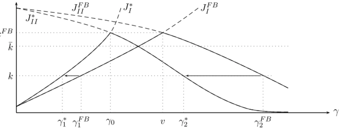
Lemma 4 For each γ there is a unique c0(γ)≤v and there is a unique γ0 ≤v given by14
v =c0(γ) +h(γ), v =γ0+h(γ0), (17) 14
such that the optimal implementation probabilities in the solution to the unconstrained version of problem R are given by
q∗(γ, c) = 1 if c≤c0(γ) 0 if c > c0(γ) , q¯∗(γ) = 1 if γ ≤γ0 0 if γ > γ0 . (18)
Lemma 4 reveals the typical distortions that are implied by the rent–efficiency trade–off that the principal faces. Observe that the second best (expected) cost thresholds γ0 and c0(γ) are
both smaller than the first–best cost threshold v. Hence, the principal distorts the
implemen-tation probabilities downwards relative to the first–best. The downward distortion lowers the information rent the principal needs to concede to the agent, because it reduces the extent to which a relatively efficient type could gain by mimicking a relatively inefficient type.
The second step is to determine the optimal information acquisition probabilities. Similarly to the first–best, the purpose of information acquisition is to prevent type I or type II imple-mentation errors. Indeed, suppose that the principal implements the project in the absence of further information. In this case her payoff is v −γ −h(γ). If information is available, the project is implemented if costs are smaller than c0(γ) in which case the principal obtains the
payoffv −c+ψ(γ, c)h(γ). Thus, the principal’s (gross) value of information is
J∗ I(γ) ≡ Z c0(γ) −∞ v−c−h(γ)dG(c|γ)−[v−γ−h(γ)] (19) = Z ∞ c0(γ) (c+h(γ)−v)dG(c|γ), (20)
where we have used that v −γ −h(γ) = R∞
−∞v −c−h(γ)dG(c|γ). Expression (20) reveals
that, due to information rents, the principal’s value of information is distorted relative to the first–best: From the principal’s perspective, a type I error occurs ifvirtual costs, c+h(γ), are larger thanv, whereas from a first–best perspective, it occurs if true costs, c, are larger than v. Note that the definition (17) implies thatc0 is non–increasing inγ becauseh is non–increasing
inγ andc. Moreover, h is non–decreasing so that the first order stochastic dominance ranking
of {G(· |γ)}γ implies that JI∗(γ) is increasing.
Similarly, suppose that in the absence of information acquisition, the principal cancels the project. In this case, information acquisition prevents a type II error whenever the value of the project v exceeds the virtual costsc+h(γ), and the principal’s (gross) value of information is
JII∗ (γ)≡
Z c0(γ)
−∞
Because h is non–decreasing and c0 is non–increasing, the first order stochastic dominance
ranking of {G(· |γ)}γ implies that JII∗ (γ) is decreasing.
According to Lemma 4, the principal executes the project without additional information exactly when γ ≤γ0. Consequently, the principal’s (gross) value of information is
J∗(γ)≡ J∗ I(γ) if γ ∈[0, γ0] J∗ II(γ) if γ ∈(γ0,¯γ]. (22)
Notice that J∗ is continuous in γ =γ
0.15 Moreover, since JI∗ is increasing and JII∗ decreasing,
J∗(γ) is single–peaked with a maximum at γ
0 of
k∗ ≡J∗(γ0) =
Z c0(γ0)
−∞
(v−c−h(γ0))dG(c|γ0).
Information acquisition by an agent typeγ is optimal for the principal if and only ifJ∗(γ)≥
k. Since J∗ is at most k∗, information acquisition is never optimal if k ≥ k∗. If k < k∗, then
single–peakedness of J∗ implies that there are exactly two cut–offsγ∗
1 < γ0 < γ2∗, which satisfy
J∗(γ1∗) = k, J∗(γ∗2) =k. (23)
Thus, it is optimal to induce information acquisition if γ ∈ [γ∗
1, γ2∗]. The following lemma
summarizes these results.
Lemma 5 The optimal information acquisition probabilities in the solution to the uncon-strained version of problemR are given as follows:
(i) If k < k∗, then α∗(γ) = 1 if γ ∈[γ∗ 1, γ2∗] 0 if γ 6∈[γ∗ 1, γ2∗] . (24)
(ii) If k ≥k∗, then α∗(γ) = 0 for all γ.
5.2
Solution to the constrained problem
We now address the question whether our solution to the relaxed version ofR actually satisfies
the constraints (AS1) and (MON2). In static problems, this simply amounts to checking a
15
monotonicity condition, which in turn is guaranteed by a monotone hazard rate. Recall from our earlier discussion that in a sequential screening problem, the first period adverse selec-tion constraints (AS1), in general, cannot be characterized in terms of monotonicity. It turns out, however, that what prevents such a characterization is that contracts are allowed to be
stochastic. In fact, our next result demonstrates that fordeterministic contracts, (AS1) can be
characterized by a monotonicity condition.16 Since the solution to the unconstrained problem
is deterministic, this implies that it also solves the constrained problem.
We define a contract as deterministic when the decision to implement the project and the
information acquisition recommendation are deterministic: α,q, q¯ ∈ {0,1}. We say that a
deterministic allocation (α,q, q¯ ) is non–increasing if there are γ1, γ2 with γ1 ≤ γ2 and a non–
increasing cutoff ˆc0 : [γ1, γ2]→R such that
α(γ) = 1 if γ∈[γ1, γ2] 0 if γ6∈[γ1, γ2] , q¯(γ) = 1 if γ < γ1 0 if γ > γ2 , q(γ, c) = 1 if c≤cˆ0(γ) 0 if c >ˆc0(γ). (25) We call an allocation that satisfies (25) non–increasing because it implies the
monotonic-ity condition (MON2) and because the expected implementation probabilmonotonic-ity α(γ)¯q(γ) + (1−
α(γ))R∞
−∞q(γ, c)dG(c|γ) is non–increasing in γ. The following lemma states our
characteriza-tion result for deterministic contracts.
Lemma 6 There are transfers (¯t, t)such that a deterministic contract (α,¯t,q, t, q¯ )satisfies the adverse selection constraints (AS1) and (MON2) if and only if (α,q, q¯ ) is non–increasing.
Because our solution to the relaxed version of R displays a deterministic, non–increasing
allocation, the lemma implies that transfers exist so that the corresponding contract satisfies (AS1) and (MON2).
Proposition 2 There are transfers(¯t∗, t∗) such that the contractC∗ = (α∗,¯t∗,q¯∗, t∗, q∗) solves
problemR and is, therefore, optimal.
5.3
Option contracts
In this subsection, we show that the implied transfers of Lemma 6 allow a reinterpretation of the contract as a menu that gives the agent the choice between a fixed price contract and
16
various option contracts. Consequently, any deterministic, direct mechanism that satisfies the adverse selection constraints can also be implemented by an indirect, empirically more natural contract. This is true in particular of the optimal contract C∗.
To demonstrate this, we first show how the adverse selection constraints pin down transfers in Lemma 6. Consider first the range of agent types who do not acquire information. Since all types in (γ2,¯γ], do not execute the project, (AS1) implies that all these types have to get
the same transfer. If the individual rationality constraint is binding, this transfer is zero. On the other hand, all types in [0, γ1) execute the project with certainty. Therefore, (AS1) implies
that transfers have to be the same for all types in [0, γ1), say ¯t. Hence, the first period adverse
selection constraints (AS1) imply that the transfer schedule ¯t(γ) exhibits
¯ t(γ) = ¯ t if γ < γ1 0 if γ > γ2. (26)
Next, consider an agent type γ who acquires information. The transfer t(γ, c) is now pinned
down by the second period adverse selection constraints (AS2). Indeed, the project is executed if the cost realization c is smaller than the cutoff ˆc0(γ). Thus, (AS2) implies that all cost
types c ≤ ˆc0(γ) who exceute the project have to get the same transfer, say t0(γ). Similarly,
all cost types who abandon the project (c > ˆc0(γ)) have to get the same transfer, say t1(γ).
Moreover, the critical cost type ˆc0(γ) has to be indifferent between executing and abandoning
the project. Otherwise, some types close to ˆc0(γ) would have incentives to lie. This pins down
the difference between t0(γ) and t1(γ) so thatt1(γ) =t0(γ) + ˆc0(γ). Hence, the second period
adverse selection constraints (AS2) imply that the transfer schedule t(γ, c) exhibits
t(γ, c) = t0(γ) if c >ˆc0(γ) t0(γ) + ˆc0(γ) if c≤ˆc0(γ). (27)
Finally, the levels of t0 and ¯t are pinned down by the condition that the boundary type γ1
(resp. γ2) has to be indifferent between acquiring information and implementing (resp. not
implementing) the project without acquiring information. If this was not the case, there would
be types close to γ1 (resp. γ2) with an incentive to misreport. Observe that in pinning down
transfers, we employed thelocal adverse selection constraints only, that is, that no type mimics a type close by. The proof of Lemma 6 shows that with a deterministic, non–increasing allocation these transfers actually satisfy the adverse selection constraints globally.
The shape of transfers allows the principal to implement the direct contract indirectly through a menu of contracts that consists of a fixed price contract and a range of option contracts. To see this, consider first what happens if the agent announces a type who does
not acquire information. Announcing γ > γ2 simply amounts to rejecting the contract, as it
entails not executing the project and zero transfers. Announcing γ < γ1 amounts to picking a
fixed price contract which obliges the agent to complete the project at all cost circumstances
for the price ¯t. Next, consider what happens if the agent announces a type who does acquire
information. After his first reportγ, the agent subsequently faces a choice between announcing
a type c >cˆ0(ˆγ) or a type c ≤ ˆc0(ˆγ). In the first case, the project is canceled and the agent
receives t0(ˆγ), while in the second case the project is implemented and the agent receives
t0(ˆγ) + ˆc0(ˆγ). Hence, effectively the agent receives the transfer t0(ˆγ) upfront and then has two
options: walk away or complete the project for the price ˆc0(ˆγ).
It consequently follows that the outcome of the optimal direct mechanism C∗ is also
im-plemented by the indirect menu contract C′ ≡ {(α = 0,¯t∗),(α = 1, c
0(γ), t∗0(γ))γ∈[γ∗
1,γ2∗]}.
The menu consists of the fixed price contract (α = 0,¯t∗) and a range of option contracts
(α= 1, c0(γ), t∗0(γ))γ. We summarize this discussion in the next proposition for the non–trivial case k < k∗.17
Proposition 3 If k < k∗, then the outcome under the optimal contract C∗ also obtains with
the contract C′ ={(α∗ = 0,¯t∗),(α∗ = 1, c
0(γ), t∗0(γ))γ∈[γ∗
1,γ2∗]}.
5.4
Distortions in information acquisition
We next investigate the distortions in information acquisition. Recall that the principal, instead of maximizing overall surplus, is only interested in the share of the surplus that she can extract. Due to asymmetric information, the principal must leave a part of the surplus — the information rents — to the agent, and consequently she is also interested in how the amount of information
acquisition affects the size of these rents. We now show that this information rent effect is
intimately linked to the type of errors that information acquisition is meant to prevent. This allows us to identify the unambiguous direction of the distortions and develop a straightforward intuition for them.
17
First, suppose that information acquisition is used to prevent type I errors. In this case, the social value of information is JIF B(γ) while the value to the principal is JI∗(γ). Because
h(γ)≥0 andc0(γ) =v−h(γ)< v, it follows JIF B(γ) = Z ∞ v (c−v)dG(c|γ) (28) ≤ Z ∞ v (c−v+h(γ))dG(c|γ)≤ Z ∞ c0(γ) (c−v+h(γ))dG(c|γ) (29) = JI∗(γ). (30)
The inequality shows that the principal overvalues information acquisition relative to the first best. That is, for preventing type I errors there is a positive information rent effect which increases the principal’s value above the first best value of information.
The intuition is as follows. When additional information prevents type I errors, some projects are turned down that would otherwise have been implemented. This means that, from an ex ante perspective, information acquisition reduces the implementation probability
q. A reduction in q for some cost type implies that, from a period 1 perspective, it becomes
less worthwhile for a more efficient cost type to mimic this cost type. Hence, the principal has to pay lower information rents to the more efficient cost types when inducing information acquisition. As a result, the optimal contract displays excess information acquisition to prevent type I errors: γ∗ ≤γF B
1 .
Next, suppose information acquisition is used to prevent type II errors. In this case, the social value of information is JF B
II (γ) and the value to the principal is JII∗ (γ). Because of
h(γ)≥0 andc0(γ) =v−h(γ)< v, it now follows
JF B II (γ) = Z v −∞ (v−c)dG(c|γ) (31) ≥ Z v −∞ (v−c−h(γ))dG(c|γ)≥ Z c0(γ) −∞ (v−c−h(γ))dG(c|γ) (32) = JII∗ (γ). (33)
The inequality shows that the principal undervalues information acquisition relative to the first best. That is, for preventing type II errors there is a negative information rent effect which decreases the principal’s value below the first best value of information.
Although the sign of the information rent effect is now negative, the intuition behind the result follows from the same logic. When additional information prevents type II errors, some
γ J∗ I JIF B J∗ II JF B II kF B γ0 v k γF B 1 γ2F B γ1∗ γ∗2 ¯ k
Figure 2: Distortions in information acquisition
projects are implemented that would otherwise have been canceled. Hence, from an ex ante
perspective, information acquisition increases the implementation probability q, and so the
principal has to pay higher information rents to the more efficient cost types when inducing information acquisition. As a result, the optimal contract displays too little information ac-quisition to prevent type II errors: γ∗
2 ≤ γ2F B. We summarize this key result in Proposition
4.
Proposition 4 Under the optimal contract, information acquisition is distorted so that there is excess (resp. insufficient) information acquisition to prevent types I (resp. type II) errors:
γ1∗ ≤γ1F B and γ2∗ ≤γ2F B.
Figure 2 illustrates the distortions. The curve J∗
I lies higher than the curve JIF B, whereas the curve J∗
II lies below the curve JIIF B. This implies that for a given k, the set of types who
acquire information the second–best, [γ∗
1, γ2∗] lies to the left of the set of types who acquire
information in the first–best, [γF B
1 , γ2F B]. It further shows how the two sets shrink as k rises.
As of ¯k the sets [γ∗
1, γ2∗] and [γ1F B, γ2F B] are disjoint: none of the types who acquire information
in the second best acquire information in the first best. This demonstrates that distortions may lead to qualitatively different outcomes.
6
Unobservable information acquisition
In this section, we examine the case when information acquisition is unobservable, and thus the optimal contract must also satisfy the moral hazard constraints (MH). The two key questions are whether the moral hazard problem causes the principal additional agency costs and how this affects distortions. We proceed in two steps. We first characterize when the optimal contract with observable information acquisition automatically satisfies (MH). Whenever this
is the case, we say that the moral hazard problem does not cause additional agency costs. In
the second step, we discuss how the optimal contract changes when the moral hazard problem causes additional agency costs and affects distortions.
Because subsequent results depend crucially on the conditional cost distributions G(c|γ), there is a loss in restricting attention to the independent case. For this reason, we now consider
more general distributions G for which the informativeness measure ψ(γ, c) is no longer
stant. In order to extend Lemma 4 to more general distributions, we impose the regularity con-ditions that∂ψ/∂c·h <1 and thatψ is non–increasing inγ. The proof of Lemma 4 shows that the first condition guarantees a unique cost typec0(γ) that solvesv−c0(γ)+ψ(γ, c0(γ))h(γ) = 0.
The second condition then implies thatc0(γ) is non–increasing inγ.18 Since{G(c|γ)}γ is ranked by first order stochastic dominance, ψ(γ, c) is negative. Finally, we require that for all γ ∈Γ:
Z ∞
−∞
ψ(γ, c)dG(c|γ) =−1. (34)
This is only a mild, technical condition. It is satisfied for any family of distribution functions
with bounded support and, therefore, is a natural continuity requirement.19 It guarantees that,
similar to (22), the value of information J∗ is the respective integral over the virtual surplus.
6.1
Agency costs through moral hazard
We turn to the question when the optimal contract with observable information acquisition,
C′, automatically satisfies the moral hazard constraints (MH). In what follows we refer toC′
18
Differentiating the identity with respect toγ yields: c′
0(1−∂ψ/∂c·h) =∂ψ/∂γ·h+ψ·h′. Hence, c′0≤0. 19
For this reason, a sufficient condition for (34) is thatG(c|γ) converges fast enough to 1 as c →+∞ and fast enough to 0 asc→ −∞. It then follows by integration by part: R∞
−∞ψ(γ, c)dG(c|γ) = ∂ ∂γ R∞ −∞G(c γ)dc= ∂ ∂γ[cG(c|γ)]∞−∞−∂γ∂ R∞ −∞c dG(c|γ) =−1.
as the benchmark contract. For the non–trivial case k < k∗, we provide two conditions for
the benchmark contract to satisfy (MH), one in terms of transfers and one in terms of the
informativeness measure ψ.
We first establish two straightforward necessary conditions on the cutoff c0(γ) and transfers
¯
t∗ and t∗
0(γ) so that the moral hazard problem does not cause additional agency costs. The
first condition is that t∗
0(γ)≤0 for all γ ∈[γ1∗, γ2∗]. The condition is necessary, because ift∗0(γ)
were strictly positive for some γ, then a type γ′ ≥ γ∗
2, instead of rejecting the contract and
receiving zero, would have a strict incentive to announce type γ in order to receive the upfront
transfer t∗
0(γ) > 0 and, subsequently, quit the project without acquiring information. The
second condition is that the net transfer when executing the project must not be higher than the transfer under the fixed price contract, that is, ¯t∗ ≥c
0(γ) +t∗0(γ) for all γ ∈ [γ∗1, γ∗2]. The
condition is necessary, because if ¯t∗ were smaller thanc
0(γ) +t∗0(γ) for someγ, then a relatively
efficient type γ′ < γ∗
1 would have a strict incentive to report type γ rather than his true type
γ′ and then, without acquiring information, choose the option to implement the project. This
strategy would allow him to complete the project for an overall transfer c0(γ) +t∗0(γ) instead
of the lower transfer ¯t∗.
We now argue that these two conditions are not only necessary but also sufficient for the moral hazard problem to not cause additional agency costs. To show sufficiency, it remains to
be checked that an agent type, γ ∈ [γ∗
1, γ2∗], who is supposed to acquire information actually
does so. There are two deviations to consider. First, suppose that such an agent type picks an option contract but deviates by quitting the project without acquiring information. The
deviator ends up with the non–positive transfer t∗
0(γ) and rejecting the contract would be a
weakly better deviation. But since C′ is individually rational, rejecting the contract cannot
be profitable. Second, suppose that an agent type γ ∈ [γ∗
1, γ2∗] picks an option contract but
deviates by completing the project without acquiring information. If this deviation is profitable, then, due to ¯t∗ ≥ c
0(γ) +t∗0(γ), an even more profitable deviation is to pick the fixed price
contract. But because the benchmark contract satisfies the adverse selection constraints (AS1), this second deviation is also not profitable. Thus, we have established:
all γ ∈[γ∗
1, γ2∗]:
¯
t∗ ≥c0(γ) +t∗0(γ) and t∗0(γ)≤0. (35)
While intuitive, the previous condition has the drawback that it depends on transfers which are endogenous. In the next lemma, we, therefore, give a sufficient condition that is only based on the primitive ψ.
Lemma 8 If ∂ψ/∂c < 0, then the moral hazard problem causes additional agency costs. If
∂ψ/∂c≥0, then the moral hazard problem does not cause additional agency costs. In particular, the moral hazard problem does not cause additional agency costs in the independent case.
Lemma 8 shows that the sign of the partial derivative∂ψ/∂cdetermines whether or not the
moral hazard problem causes additional agency costs. We shall explain the intuition behind this result in detail, as it will guide us in constructing the optimal contract when the moral hazard problem causes additional agency costs.
Intuitively, the agent has an incentive to acquire information when his value of information
exceeds acquisition costs k. Note that when the agent chooses an option contract, information
is valuable to the agent, because the contract allows him to choose the best option according to true cost conditions. Hence, the crucial question is to what extent the agent’s value of information coincides with the principal’s. To answer this, consider the value of information to some agent typeγ. Given an option contract, typeγ’s next best alternative without information is either to execute the project for a price p = c0(γ) or to quit the project. Under the first
alternative, an informed type γ saves p−c when the additional information reveals that the
cost cexceeds p. Therefore, the agent’s value of information in this case is
JA
I (p, γ) = Z ∞
p
c−p dG(c|γ), (36)
where, under the benchmark contract,pequals c0(γ). When the next best alternative is to quit
the project, an informed type γ gains p−c when the additional information reveals that the
cost cis smaller than the price p. Hence, the agent’s value of information in this case is
JA
II(p, γ) = Z p
−∞
Now, the moral hazard problem does not cause additional agency costs when the agent’s value of information is sufficiently large. More precisely, suppose that the agent typeγ’s value
of information is larger than k whenever the principal’s value of information J∗(γ) is also
larger than k. In that case, the agent’s and the principal’s incentives to acquire information
are aligned, and the agent voluntarily acquires information. Hence, if JA
I (c0(γ), γ) ≥ k and
JA
II(c0(γ), γ)≥k for all γ ∈[γ1∗, γ2∗], then there are no additional agency costs.
In order to see that the sign of ∂ψ/∂c determines whether this is the case, consider a
situation where both the principal’s and the agent’s best alternative without information is to abandon the project. In that case, the principal’s value of information is her virtual valuation integrated over the cost rangec < c0(γ) while the agent’s value of information is his “gross ex
post rent”c0(γ)−cintegrated over the same range. Now observe that both the virtual surplus
and the gross ex post rent are exactly zero at c0(γ), and in the range c < c0(γ) the ex post
gross rent increases at a rate of +1 as cbecomes smaller, while the principal’s virtual surplus
increases at the rate of 1−∂ψ/∂c·h. Hence, for the independent case ∂ψ/∂c= 0, these rates
coincide and therefore also the agent’s and the principal’s value of information. For∂ψ/∂c >0, the agent’s value of information is actually larger than the principal’s so that the agent has a strict incentive to acquire information whenever the principal wants him to do so. If, on the
other hand, ∂ψ/∂c < 0, then the principal’s value of information is larger than the agent’s.
In that case, incentives for information acquisition are misaligned for some types γ, and the
benchmark contract has to be adapted to account for the moral hazard problem. We now turn to this issue.
6.2
Optimal contract when moral hazard causes agency costs
Finding the optimal contract when the moral hazard problem causes additional agency costs is complicated in general because the adverse selection constraint cannot be characterized in terms of monotonicity. However, as shown in Lemma 6, for deterministic contracts such a characterization is possible. This will allow us to solve the problem when we restrict attention to deterministic contracts. In light of Lemma 6, we can associate with any deterministic contract that satisfies the adverse selection constraints a non–increasing cutoff ˆc0 : [γ1, γ2]→R. Recall
where the option price to execute the project coincides with the cutoff cˆ0(γ). In what follows,
we therefore use the terms price and cutoff interchangeably.
With deterministic contracts there are, in effect, two ways how to modify the benchmark contract when it violates the moral hazard constraints. First, the principal could limit infor-mation acquisition to those agent types whose value of inforinfor-mation is already high enough. In this case, additional agency costs arise since information acquisition sometimes does not take
place even though the principal’s value of information exceeds k. The other possibility is to
adapt the price p = c0(γ) so as to raise the agent’s value of information. Due to incentive
compatibility, a price increase (resp. decrease) means, however, that the agent executes (resp. abandons) projects with a negative (resp. positive) virtual surplus. Hence, additional agency costs also arise from this second possibility. The intuitive idea for finding the optimal contract is to adapt the information acquisition interval and the price so that the two different types of agency costs are optimally balanced.
We now formalize this idea. We first characterize all prices that give agents a positive incentive to acquire information and look for the optimal price in this set. Given these optimal prices, we can then determine the optimal range of information acquisition [γ1, γ2]. We begin by
showing that prices that induce information acquisition by the agent lie between two bounds,
pI and pII. Recall from (36) and (37) that confronted with a price p, the agent acquires
information if both JA
I (p, γ) and JIIA(p, γ) are larger than k; otherwise he would be better off by taking the next best alternative without information. We have:
Lemma 9 Let i=I, II.
(i) For each γ, there is a unique solution pi(γ) to JiA(p, γ) =k.
(ii) pi is increasing in γ.
(iii)JA
I (p, γ)≥k if and only if p≤pI(γ), and JIIA(p, γ)≥k if and only if p≥pII(γ).
Lemma 9 implies that the set of prices for which the agent has a positive incentive to acquire
information is the band between the two pi–curves:
P ≡ {(γ, p)|pII(γ)≤p≤pI(γ)}. (38)
We can now provide a characterization analogous to Lemma 6 which includes the moral hazard constraints. The additional requirement is that the endpoints of ˆc0 are inP.
Lemma 10 There are transfers (¯t, t) such that a deterministic contract (α,¯t,q, t, q¯ ) satisfies the adverse selection constraints (AS2), (AS1) and the moral hazard constraints (MH) if and only if (α,q, q¯ ) is non–increasing and
(γ1,ˆc0(γ1)),(γ2,ˆc0(γ2))∈P. (39)
As explained earlier, the moral hazard constraints are satisfied if the whole schedule ˆc0 is
in P. The reason why we only have to consider the endpoints is that the two pi-curves are
increasing, whereas ˆc0 is necessarily non–increasing.
Restricting attention to deterministic contracts, we can now treat problem P as usual.
By Lemma 1 and 2, the agent’s utility U is given by (14) and, therefore, decreasing in γ.
Optimality then requires that the individual rationality constraint is binding for the highest
type ¯γ. Together with (14), this pins down the agent’s utility, which we can then insert in
the principal’s objective. Integration by parts transforms the principal’s objective into the expected virtual surplus as stated in (15). Finally, by Lemma 10 and exploiting the structure of a non–increasing allocation (α,q, q¯ ) we can restate the problemP as follows.
S : max γ1,γ2,ˆc0 Z γ1 0 v−γ−h(γ)dF(γ) + Z γ2 γ1 [ Z ˆc0(γ) −∞ v−c+ψ(c, γ)h(γ)dG(c|γ)−k]dF(γ)(40) s.t. (39) and ˆc0 : [γ1, γ2]→R is non–increasing.
We can find a solution to S by the following two–step procedure: First, determine the
opti-mal price schedule ˆc0 for given thresholds γ1 ≤ γ2 and, subsequently, determine the optimal
thresholdsγ1 and γ2 by optimizing over all optimal price schedules ˆc0. We call ˆc0 optimal with
respect to a pair (γ1, γ2) if ˆc0 is a solution ofS for given thresholds γ1 and γ2. The next lemma
characterizes the optimal price schedule ˆc0 given a pair (γ1, γ2).
Lemma 11 The price schedule ˜c0 is optimal with respect to a pair (γ1, γ2) where
˜
c0(γ)≡min{pI(γ1),max{c0(γ), pII(γ2)}}. (41)
Intuitively, the optimal schedule ˜c0 coincides with the benchmark schedule c0 whenever
γ c c0(γ) pI(γ) pII(γ) pI(γ1) pII(γ2) ˆ c0(γ) γ1∗ γ1 γ2 γ2∗
Figure 3: Bunching due to moral hazard
in between pI(γ1) and pII(γ2). Otherwise, the price has to be adapted so as to increase the
agent’s value of information. Adapting the price implies a suboptimal decision by the agent in period 2 and entails losses in virtual surplus. Hence, the optimal new price is the one closest to the original price c0(γ) among all prices that are incentive compatible, i.e. non–increasing
and in P. As illustrated in Figure 3, the optimal schedule ˜c0 can, therefore, be found by a
bunching or ironing procedure, which flattens parts of the benchmark schedule c0, leading to
price bunching for different γ types. The remaining problem is, then, to determine over which
ranges bunching takes place. The solution to this problem yields the optimal thresholdsγ1 and
γ2. While the exact optimal thresholds γ1 and γ2 depend on the details of the primitives, the
following proposition shows how the moral hazard problem affects information acquisition: Proposition 5 When the moral hazard problem causes agency costs, the range of information acquisition shrinks relative to the case with observable information acquisition:
γ1 ≥γ1∗ and γ2 ≤γ2∗. (42)
The intuition for Proposition 5 is that outside the interval [γ1∗, γ2∗], information acquisition
costs k exceed, by definition, the principal’s value of information. Hence, even if a price could
be found that induces information acquisition by agent types outside of [γ∗
1, γ2∗], this would be
suboptimal because information acquisition would cause a loss to the principal.
Proposition 5 allows us to identify the impact of the moral hazard problem on the distortions in information acquisition beyond those caused by adverse selection. When the moral hazard
problem causes agency costs, then, relative to the case with observable information acquisition, both more type I and more type II errors are committed. Hence, information acquisition to prevent type I errors become less distorted and more efficient, while information acquisition to prevent type II errors becomes more distorted and less efficient. Consequently, the welfare effects of the additional moral hazard constraints are ambiguous and it could be that the first effect outweighs the second. In this case, the presence of the moral hazard problem would actually increase overall efficiency. Because the moral hazard problem unambiguously raises the agency costs of the principal, an increase in efficiency means that the agent gains more than the principal loses.
7
Empirical Implications
In this section, we relate our theoretical analysis to some features of real world contracts and discuss testable implications of our theory. Earlier work on dynamic mechanism design already demonstrated that option contracts represent optimal contractual structures in dynamic screening problems. Classical examples of contracts with option clauses that adapt contracting terms to new information are labor contracts, securities such as put or call options, or ticket pricing. The existence of such contracts can be rationalized by straightforward reinterpretations of our model (e.g. viewing the agent as the buyer with uncertain demand and the principal as the seller). Option contracts are prevalent also in business-to-business procurement. Refund or buy–back contracts play a key role in vertical manufacturer retailer relations in which there is uncertainty (about demand or costs) during a sales period. The management literature reports the widespread use of option contracts in publishing, CD retailing (Kandel, 1996), for fashion goods such as apparel (Eppen and Iyer, 1997), in the semiconductor and consumer electronic industries (Milner and Rosenblatt, 2002), or in catalogue retailing (Donohue, 2000). In all these examples, private information and active information acquisition are often intertwined. Our results show that the prevalence of option contracts in real life can be understood as optimal contractual responses to both information acquisition and dynamic screening. Moreover, they demonstrate the robustness of the previous literature that mainly concentrated on the screening aspect.