Monetary policy shocks and
long-term interest rates
Wendy Edelberg and David Marshall
When monetary policymakers act, what happens to bond yields? There are good theo-retical reasons why shorter-term bond yields should be affected by monetary policy. Open market operations of the Federal Reserve System have an immediate effect on the federal funds rate, which is the interest rate charged for overnight interbank loans. Since short-term borrowing (such as a one-month loan) acts as a reason-ably close substitute for overnight borrowing, an increase in the federal funds rate should be accompanied by an increase in other short-term interest rates. However, it is less clear why monetary policy should have a significant effect on five-, ten-, and 15-year bond yields. It seems doubtful that five-year loans are close substitutes for overnight borrowing. Yet, casual observation suggests that monetary policy actions are associated with changes in long-term bond yields.
Consider the bond market debacle of 1994. Publications ranging from Barron’s to the Los Angeles Times argue that 1994 was the worst year for the bond market since the 1920s. In figure 1, we display the one-year holding period returns for zero-coupon bonds of four years, six years, and ten years in matu-rity.1 (The vertical lines toward the right-hand
side of each panel indicate January 1994.) If we exclude the volatile period from 1979–82 (when the Federal Reserve experimented with direct targeting of monetary aggregates), the one-year cumulative losses in late 1994 were
among the worst of the postwar period. This collapse of bond prices took its toll on well-known bond investors: Michael Steinhart’s hedge fund sustained losses of 30.5 percent in 1994, George Soros’s fell 4.6 percent, and Julian Robertson’s fell 8.7 percent—all com-ing off very strong performances in 1993.
At the same time, 1994 was a period of concerted monetary tightening. After a period during which the federal funds rate was excep-tionally low and stable, the Federal Open Market Committee (FOMC) raised the funds rate rapidly. As shown in figure 2, the 18 months from mid-1992 through the end of 1993 were characterized by a federal funds rate near 3 percent, with very little variability. This period more closely resembles the mid-1960s than the more volatile 1970s and 1980s. From February 1994 through February 1995, the FOMC doubled its target for the funds rate from 3 percent to 6 percent in seven incre-ments. Figure 2 shows that this sort of mone-tary tightening is hardly unusual (even exclud-ing the 1979–82 period, when the federal funds rate was not the monetary policy instru-ment). Nonetheless, the congruence of these two events (the rapid tightening of monetary policy and the precipitous rise in long-term Wendy Edelberg is an associate economist and David Marshall is a senior economist at the Federal Reserve Bank of Chicago. The authors thank Char-lie Evans for many useful discussions and for pro-viding his VAR estimation code. They also thank John Cochrane and Kent Daniel for helpful com-ments and Jennifer Wilson for research assistance.
bond yields) led some to assert that the col-lapse in the bond market was policy induced. For example, the Wall Street Journal of December 13, 1995 graphically describes February 1994 as the month “when the Fed began raising short-term interest rates and set off the year’s bond-market slaughter.”
In this article, we will look at the relation-ship between monetary policy and long rates during the postwar period, and then apply what we learn to the extraordinary events of 1994. To examine how a monetary policy action (such as an increase in the federal funds
rate) affects the yields of bonds with differing maturities, we must confront the problem of causality. For example, suppose we find that a tightening of monetary policy is associated with higher long-term bond yields. Can we then infer that tighter monetary policy causes higher yields? Not necessarily. It is generally believed that the FOMC tends to tighten mon-etary policy when there are indicators of future inflation. It is also believed that expectations of higher inflation tend to increase current bond yields. The positive correlation be-tween tighter money and higher yields could
FIGURE 1
One-year holding period returns
-10 0 10 20 30 40 1950 ’55 ’60 ’65 ’70 ’75 ’80 ’85 ’90 ’95 percent A. Four-year bond -15 0 15 30 45 1950 ’55 ’60 ’65 ’70 ’75 ’80 ’85 ’90 ’95 percent B. Six-year bond percent -25 0 25 50 75 1950 ’55 ’60 ’65 ’70 ’75 ’80 ’85 ’90 ’95 percent C. Ten-year bond 1/94 1/94 1/94
Sources: Authors’ calculations from McCulloch and Kwon (1993), augmented with data from theWall Street Journal, 1991-95, various issues.
FIGURE 2
Federal funds rate
0 5 10 15 20 1955 ’60 ’65 ’70 ’75 ’80 ’85 ’90 ’95 percent 1/94
Source: Federal Reserve Board of Governors (1995).
1/94
be evidence that the Fed causes yields to in-crease when it tightens money, or it could be evidence that both the Fed action and the high-er yields are jointly caused by forecasts of higher inflation.2
To help us disentangle the various possible directions of causality, we use a framework developed by Lawrence Christiano, Martin Eichenbaum, and Charles Evans in a series of working papers published by the Federal Re-serve Bank of Chicago.3 In the
Christiano-Eichenbaum-Evans (CEE) framework, a clear distinction is made between the monetary au-thority’s feedback rule and an exogenous mone-tary policy shock. The feedback rule relates policymakers’ actions to the state of the econo-my.4 In the example of the preceding paragraph,
the “normal” reaction of the Fed to an increase in inflation expectations would be incorporated into the feedback rule. The exogenous monetary policy shock is defined as the deviation of actual policy from the feedback rule. We refer to these policy shocks as “exogenous” because, by con-struction, they do not respond in any systematic way to the economic variables that are included in the feedback rule. (If certain realizations of these variables systematically implied a higher-than-average or lower-higher-than-average policy shock, then the rule is incompletely specified: Any systematic linkage between the policy-shock component and the feedback-rule compo-nent should have been loaded into the feedback rule in the first place.)
We measure monetary policy by the level of the federal funds rate. We use the CEE framework to decompose chang-es in the funds rate into the feed-back-rule component and the policy-shock component, and we ask how bond yields respond to an exogenous monetary poli-cy shock. By focusing on the policy-shock component, we resolve the problem of ambiguous causality: Since the policy shock is exogenous by construction, causality can only flow from the policy shock to the bond yields (and to the other variables in the economy). However, this resolu-tion is not without cost: We can-not ask how a change in the struc-ture of the feedback rule itself would affect the behavior of long-term bond yields. The prob-lem is that all observed economic relations are conditional on the particular feedback rule in place. [This is an application of the celebrated Lucas (1976) critique.]
To explore the consequences of a change in the feedback rule, one would have to specify a model of the bond market at the level of investor preferences, monetary policy objec-tives, technological constraints, and market structure. We do not attempt this potentially useful but extremely difficult modeling task in this article.
Once we determine the response of bond yields to an exogenous monetary policy shock, we can look at the events of 1994 through this lens: (1) To what extent was the monetary tight-ening in 1994 an application of the FOMC’s prevailing feedback rule, and to what extent did it reflect exogenous shocks to monetary policy?; and (2) To what extent did policy shocks affect long-term bond yields during this period? In particular, if there were no policy shocks (that is, if the monetary authority had followed the feedback rule exactly), would the increase in bond yields have been substantially reduced?
Below, we describe the CEE framework and how it is used to investigate the behavior of long-term bond yields. We then detail the average response of bond yields to exogenous monetary policy shocks. Our analysis indicates
that these policy shocks have a substantial impact only on short-term bond yields; the impact on maturities longer than three years is quite small, and the impact on maturities long-er than 15 years is insignificant. We considlong-er two theoretical explanations for these results: the expectations hypothesis of the term struc-ture and the Fisher hypothesis that movements in long-term bond yields reflect changes in expected inflation. We find that the response of long yields to exogenous monetary policy shocks closely follows the predictions of the expectations hypothesis, while the Fisher hy-pothesis explains very little. We then apply our methodology to the 1994 period.
A framework for analyzing the effects of monetary policy on bond yields
The model we use for exploring the effects of monetary policy shocks is the version of the CEE framework with monthly data discussed in Christiano, Eichenbaum, and Evans (1994b, section 5). We include four types of variables in our model. The first is the monetary policy instrument. We assume that this policy instru-ment is the federal funds rate. Christiano, Eichenbaum, and Evans (1994b) also explore the use of nonborrowed reserves as an alterna-tive policy instrument. They obtain stronger results with the federal funds rate, but their results are fairly robust to the choice of instru-ment. The second type of variable is contem-poraneous inputs to the feedback rule. We assume that this feedback rule incorporates contemporaneous values of the log of nonagri-cultural employment, as measured by the es-tablishment survey (EM), the log of the price level, as measured by the personal consump-tion expenditure deflator (PCED), and the change in an index of sensitive materials pric-es (CHGSMP).5 We use EM as a monthly
indicator of real economic activity. We mea-sure the price level by PCED, rather than by the consumer price index (CPI), because the CPI is a fixed-weight deflator. Christiano, Eichenbaum, and Evans (1994b) discuss cer-tain anomalous patterns that emerge when a fixed-weight deflator is used to gauge the price level.6 These patterns are less of a
prob-lem when a variable-weight measure of con-sumer prices, such as PCED, is used. Finally, the CHGSMP series is a good pre-dictor of future inflationary pressure. Some such predictor must be included if we are to
construct a plausible representation of the Fed’s feedback rule.
The third type of variable we include is the yield on a zero-coupon bond with T peri-ods to maturity (YT); we rotate, one at a time, through maturities from one month to 29 years.7 We use yields on zero-coupon bonds
to avoid complications associated with coupon payments. The yields from 1947 to 1991 are monthly data taken from J. Huston McCulloch and Heon-Chul Kwon (1993).8 For the period
1991 through 1995, we use yields on Treasury STRIPS quoted in the Wall Street Journal for the first business day of each month. Finally, we include additional explanatory variables for long-term yields. In this category of vari-ables, we use the log of nonborrowed reserves (NBR) and the log of total reserves (TR). We use these variables as measures of the demand for credit in the economy. In partic-ular, the amount of nonborrowed reserves that must be injected or withdrawn to achieve a given federal funds target is determined by the price elasticity of demand for reserves. By including total reserves as well as nonbor-rowed reserves, we measure the component of reserve demand that is accommodated through the discount window.9
The resulting model includes seven indi-vidual variables: EM, PCED, CHGSMP, FF, NBR, TR, and YT. We assume that the mone-tary policymakers’ feedback rule is a linear function of (1) contemporaneous values of EMt, PCEDt, and CHGSMPt, and (2) lagged values of all variables in the economy. That is, the Federal Reserve sets policy based on current economic activity (as measured by EMt) and price movements (as measured by PCEDt and CHGSMPt), as well as the entire history of the economy. The policy decision, in turn, has a contemporaneous effect on re-serves and bond yields and affects the future realizations of all variables in the economy. Some argument could be made for including interest rates in the feedback rule, but there is statistical and economic justification for mod-eling the influence in the other direction. Cook and Hahn (1989) find that even on a daily basis there is little evidence of system-atic movements in interest rates prior to an announcement of a change in the federal funds rate, while there are systematic movements after such an announcement.
FIGURE 3
The effect of a federal funds shock basis points A. One-month yield -16 0 16 32 48 2 4 6 8 10 12 14 16 18 20 22 24 -16 0 16 32 48 2 4 6 8 10 12 14 16 18 20 22 24 basis points D. Three-year yield -16 0 16 32 48 2 4 6 8 10 12 14 16 18 20 22 24 basis points B. Six-month yield -16 0 16 32 48 2 4 6 8 10 12 14 16 18 20 22 24 basis points E. Ten-year yield steps -16 0 16 32 48 2 4 6 8 10 12 14 16 18 20 22 24 basis points C. One-year yield -16 0 16 32 48 2 4 6 8 10 12 14 16 18 20 22 24 basis points steps F. 15-year yield
Note: For each bond, the black line traces the response path over 24 months following the shock. The colored lines above and below the response give the 95 percent confidence bands, computed by Monte Carlo simulation using 1,000 independent draws.
Sources: Calculations from authors’ statistical model, using the following data series: U.S. Bureau of Labor Statistics—employment survey measurements of nonagricultural employment (EM); U.S. Bureau of Economic Analysis—personal consumption expenditure deflator (PCED) and index of sensitive materials prices (CHGSMP); McColloch and Kwon (1993) augmented with data from Wall Street Journal 1991-95, various issues (YT); and Federal Reserve Board—federal funds rate (FF), nonborrowed reserves (NBR), and total reserves (TR).
the residuals from the equations for EM, PCED, and CHGSMP. The exogenous mone-tary policy shock is that portion of the residual in the FF equation that is not correlated with this estimated feedback rule. The technical appendix to this article describes in detail how we set up and estimate this VAR, and how we use the VAR to infer the exogenous policy-shock component of FF.
We estimate this linear feedback rule as part of a vector autoregression (VAR) system. Formally, the system consists of seven equa-tions. Each equation in the system takes one of the seven variables to be its dependent variable. For each equation, the independent variables are lagged values of all seven vari-ables. The feedback rule consists of the fitted equation for FF, plus a linear combination of
In addition to the exogenous monetary policy shock, our model incorporates exoge-nous shocks to the other six variables. That is, there are a total of seven shock processes that act as the fundamental exogenous driving cesses in the economy. These exogenous pro-cesses are transformations of the residuals from our seven VAR regressions. In particular, the exogenous shocks are serially uncorrelated, and are constructed to be mutually uncorrelated. (The technical appendix describes how we can isolate the effects of these seven exogenous processes.) Unexpected movement in any variable in the economy must be attributable to the effect of one or more of these exogenous processes. Below, we investigate how much of the unexpected movement in FF and YT can be attributed to the exogenous shocks to each of the seven variables in the model.
The response of bond yields to exogenous monetary policy shocks
Figure 3 plots the estimated responses of bond yields to a one-standard-deviation exoge-nous monetary policy shock. This corresponds to an increase in the federal funds rate of ap-proximately 50 basis points.10 We display the
responses for bond maturities of one month, six months, one year, three years, ten years, and 15 years. The colored lines delineate 95 percent confidence interval bands.11 The
plots trace the responses over 24 months. A 50-basis-point federal
funds shock increases the one-month rate by approximately 30 basis points in the period when the shock occurs. This response is highly significant statistically. The one-month rate continues to climb in the following period, and then falls, with the effect of the shock completely attenuated after 21 months. The six-month and one-year rates display qualitative-ly similar response patterns, al-though the magnitude of the re-sponse decreases for the longer-term bonds. When we move to longer-term bonds, the initial effect diminishes substantially as maturity increases: The initial response of the three-year bond is only 12 basis points, and the re-sponses of the ten- and 15-year
bonds are each less than 5 basis points. Ac-cording to the point estimates, the response of the longer-term bonds appears more per-sistent than that of the shorter-term bonds. However, this apparent persistence is not statistically significant: The initial response for the ten- and 15-year bonds is barely sig-nificant; the response to a federal funds shock of all bonds longer than 15 years is insignifi-cant at the 5 percent marginal significance level. For all maturities, the response is in-significant by one year. Interestingly, these results are roughly comparable to Cook and Hahn’s (1989) estimates of the effects on interest rates of a publicly announced change in the federal funds rate. They find that in response to a 100-basis-point increase, short rates rise about 50 basis points, while long rates rise about 10 basis points.
The results are straightforward: There is a significant and relatively large effect on the short rates, with a decreasing, less significant effect at longer maturities. The effect on the term structure can perhaps be seen more easily by plotting the effect of a contractionary shock on the yield curve. The black line in figure 4 is the average yield curve from 1990 through 1995, for maturities up to five years. The remaining lines show our point estimates for the response of the yield curve to a one-stan-dard-deviation exogenous monetary policy
FIGURE 4
The effect of a one-standard-deviation federal funds shock on the term structure
5.4 5.8 6.2 6.6 7.0 7.4 0 1 2 3 4 5 yield maturity in years
Average yield curve Initial period response Six-month response Two-year response
Sources: See figure 3.
shock after one month, six months, one year, and two years. To illus-trate the qualitative patterns more clearly over a wider range of matu-rities, figure 5 displays a similar plot for a five-standard-deviation monetary shock, with maturities up to 29 years. These plots clearly show that the impact on the term structure is a rise in shorter rates, with the effect diminishing as maturities increase. In other words, a monetary policy shock raises the level, flattens the slope, and decreases the curvature of the yield curve.
Why do monetary policy shocks affect yields? What gener-ates the observed response in yields of different maturities to a monetary policy shock? We con-sider two well-known hypotheses:
the expectations hypothesis, which states that the long yield is an average of expected future short yields, and a version of the Fisher hy-pothesis, which states that changes in long yields are largely determined by changes in expected inflation.
The expectations hypothesis
The expectations hypothesis can be written 1)
Equation 1 says that the long yield, YtT, on a T-period zero-coupon bond is the average of expected future yields on one-period bonds over the next T periods, plus a time-invariant term premium, TPT. The expectations hy-pothesis is attractive, because it implies that changes in forward interest rates should pro-vide unbiased forecasts of changes in future spot rates. Unfortunately, tests of equation 1 using postwar U.S. data tend to decisively reject the hypothesis. For example, the equa-tion implies that changes in the term spread YtT – Y
t
1 should predict future yield changes
Yt+1T–1 – Y t
T. That is, in the following regression
2)
FIGURE 5
The effect of a five-standard-deviation federal funds shock on term structure
5.2 5.8 6.4 7.0 7.6 8.2 0 4 8 12 16 20 24 28 yield maturity in years
Average yield curve
One-year response Initial period response Six-month response
Sources: See figure 3.
Two-year response = T 1
Σ
EtY1 t+i + TP T. YtT YT–1 – YT t = a + b [Y T t – Y 1 t] + et +1 t+1the slope coefficient b should equal unity. Campbell and Shiller (1991) show that, for numerous data samples and numerous maturi-ties T, this slope coefficient is significantly negative. McCallum (1994) suggests that the Campbell-Shiller regressions may be problem-atic econometrically in the presence of activist monetary policy. If the term premium TPT displays only a small degree of time variation (so the expectations hypothesis holds approxi-mately), but the monetary authority observes and responds to this time variation in TPT, then et+1 may be correlated with YtT – Y
t
1. This
could bias the slope coefficient b downward. McCallum gives examples where the resulting bias is sufficient to explain the Campbell-Shiller results.
In our impulse response functions, the expectations hypothesis would predict that the one-step-ahead response of YtT should equal the average of the first T-period-ahead responses of the short rate Yt1. The
Camp-bell-Shiller results suggest that the expecta-tions hypothesis may perform poorly as an explanation of our impulse responses. On the other hand, our framework may not be vulnerable to McCallum’s critique, since we model monetary policy explicitly. If the variables entering the feedback rule include those variables that shift the term premium, t–1
i=0
T–1 1
of its effect on the expected future price level: The first-period response of YtT should equal the T-period-ahead re-sponse of the price level PCEDt.
There is substantial evidence against a literal one-to-one rela-tionship between changes in expected inflation and changes in shorter-term interest rates.13
However, it is not implausible that fluctuations in expected inflation are reflected, at least in part, in longer-term bond yields. To investigate this idea within our framework, we ask how much of the response of long yields to a monetary shock can be explained by the corresponding response in expected inflation. That portion of the response that cannot be tied to expected infla-tion would be attributable to liquidity effects, of the type described in Chris-tiano and Eichenbaum (1992).
We assume that the impulse response of the price level is a good proxy, under rational expectations, for expected inflation following a shock in monetary policy. In figure 7, we display the response of our measure of the price level, PCED, to a one-standard-devia-tion contracone-standard-devia-tionary shock to monetary policy. In figure 8, we display the difference be-tween the first-step response of YtT and the T-step-ahead response of PCEDt, divided by T in years, for maturities T ranging from two months through fifteen years. Unlike the expectations hypothesis, the Fisher hypothe-sis offers little explanation for our impulse responses. For all maturities, the difference between the first-period response of the bond yields and the response predicted by the Fish-er hypothesis is significantly diffFish-erent from zero. Furthermore, the point estimates of these differences are fairly large, between 10 and 20 basis points. To see the source of this failure, compare figure 7 with figure 3. Figure 7 displays the response of the price level PCED to a one-standard-deviation mon-etary policy shock, along with the 95 percent confidence intervals. Initially, a monetary contraction is followed by a small (barely FIGURE 6
Expectations hypothesis
then our regressions will not display the McCallum bias.
In figure 6, we display the difference between the first-step response of YtT and the average of the first T-step responses of Yt1,
for T ranging from two months through 15 years. (The methodology used to con-struct the confidence intervals is described in the technical appendix.) According to this figure, the expectations hypothesis does a good job of explaining the impulse-response patterns. For all maturities, the difference between the first-period response of the long bond and the response predicted by the ex-pectations hypothesis is less than 6 basis points, and is insignificant at the 5 percent marginal significance level.
The Fisher hypothesis
There is a school of thought that a good deal of the variation in very long-term bond yields is due to changes in expected inflation. An extreme version of this idea is the Fisher hypothesis, which asserts that the nominal bond yield YtT should move, one for one, with changes in inflation expected over the life of the bond (that is, over the next T periods.)12
Under this hypothesis, the only reason a mone-tary shock should affect long yields is because
-15 0 15 30
0 1 2 3 4 5 6 7 8 9 10 11 12 13 14 15 difference in basis points
maturity in years
Note: For maturities T ranging from two months through 15 years, the black line plots resp1 (YT
) – ΣTi=1 respi, (Y1), where respi (Yj ) denotes the response of Yt +i (the yield on a j-period bond in period t+i ) to aj one-standard-deviation exogenous monetary policy shock in period t. The colored lines display 95 percent confidence bands.
Sources: See figure 3. T 1
policy shock is positive. We find essentially no evidence that the response of long yields to an exogenous monetary shock is due to that shock’s effect on expectations of future inflation.
In summary, we find that a contractionary exogenous shock to monetary policy has a strong upward impact on the one-month rate. One-one-month loans are a partial substitute for over-night borrowing, so it would be surprising if the one-month rate did not respond strongly to an increase in the federal funds rate. The impact of a shock to monetary policy on longer-bond yields declines with maturity, with this decline well explained by the expectations hypothesis. That is, the declining impact of a monetary policy shock on longer-maturity yields tracks the rate at which the response of the one-month yield attenuates. We find no evidence of an excessive response of long yields to monetary innovations. At the same time, changes in expected inflation do not appear to account for the observed responses.
Monetary policy and bond yields in 1994
We use the results from the model to examine the behavior of monetary policy and the bond markets in 1994. Taking the VAR estimates as given, we decompose the movement of the federal funds rate and bond yields into the following: (1) the expected path, given information known in December 1993; (2) the unexpected move-ment attributable to the exoge-nous monetary policy shocks; and (3) the unexpected move-ment attributable to exogenous shocks to the other variables in the economy.
We first look at the deter-minants of the federal funds rate. Panel A of figure 9 shows FIGURE 7
The effect of a fed funds shock on the price level
FIGURE 8
The Fisher hypothesis
T ranging from two months through 15 years, the black line ( ) T
Note: For maturities plots T(yrs)
1
respT denotes
t+i
the response of to a one-standard-deviation exogenous shock to
monetary policy in periodt. The colored lines display 95 percent confidence bands. resp1Y , where for any variableX, resp (X)i
-10 0 10 20 30 40 0 1 2 3 4 5 6 7 8 9 10 11 12 13 14 15
difference in basis points
maturity in years
(PECD) X
Sources: See figure 3.
significant) rise in the price level.14 The
price level eventually falls in response to a monetary policy shock. Under the Fisher hypothesis, this would imply a negative response of the longer-maturity yields to a monetary contraction. However, the esti-mated response of all yields to the monetary
-3 -2 -1 0 1 0 20 40 60 80 100 120 140 160 180 200 percent steps
Note: The black line represents the response to an exogenous monetary policy shock. The colored lines represent 95 percent confidence bands. Sources: See figure 3.
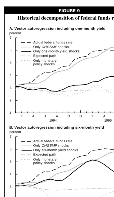
the decomposition of the federal funds rate when the VAR includes the one-month yield. Panel B shows the analogous decomposition when the VAR includes the six-month yield.15 For both models, the expected path
for the federal funds rate is flat. In contrast, the actual federal funds rate rises approxi-mately 300 basis points from January 1994 through April 1995.
What accounts for this dramatic, unex-pected tightening of monetary policy? By construction, the only sources of unexpected movements in the monetary policy are the exogenous policy shocks, and the effect of other economic shocks acting through the
feedback rule. Figure 9 shows the relative importance of these two components. According to panel A of figure 9, the policy shocks account for virtually none of the unexpected run-up in the federal funds rate. Panel B of figure 9 indicates the exoge-nous policy shocks actually pull the federal funds rate below the expected path. It follows, there-fore, that the increase in the federal funds rate must be due to the workings of the feedback rule. In particular, figure 9 indicates that most of the move-ment in the federal funds rate above the baseline forecast represents a response of the feedback rule to unexpected increases in sensitive materials prices. In both panels of figure 9, the line giving the path of the federal funds rate that would have obtained if all shocks other than shocks to CHGSMP were set equal to zero is very close to the path actually observed.
Recall that lagged values of the bond yield enter the feed-back rule for monetary policy. Figure 9 documents the effect of shocks to the bond yield on the path of the federal funds rate. With the one-month bond (panel A of the figure), the exogenous shocks to the one-month yield have a rather small effect on the funds rate. When the six-month yield is used (panel B), the exogenous shocks in the bond yield do tend to push the funds rate above the expected path, but this effect is largely offset by the estimated exogenous monetary policy
shocks.16 The contributions from the inputs to
the monetary policy rule other than the bond yield and CHGSMP are relatively small, so they are not plotted in figure 9.
Our analysis indicates that the rise in the federal funds rate during 1994 and the first few months of 1995 was largely a mechanical response of the feedback rule to an increased FIGURE 9
Historical decomposition of federal funds rate
1 2 3 4 5 6 7 F A J A O D F A J A percent 1994 1995
A. Vector autoregression including one-month yield
1 2 3 4 5 6 7 F A J A O D F A J A percent 1994 1995
B. Vector autoregression including six-month yield
Actual federal funds rate
Only monetary policy shocks Expected path Only
Only one-month yield shocks
Actual federal funds rate
Only monetary policy shocks Expected path
Only six-month yield shocks
Sources: See figure 3.
CHGSMPshocks
15-year yield. However, virtual-ly none of this increase can be attributed to exogenous mone-tary policy shocks. In figure 11, we plot the path of each yield that would have obtained if the feedback rule were followed strictly. (That is, if the exoge-nous monetary shocks were all set equal to zero.) For each bond, the path is virtually un-changed.
We can use our VAR model to explain the deviation of the bond yields from their expected paths. While some of these unexpected yield changes are a result of exogenous shocks to changes in sensitive materials prices (and, to a lesser degree, the remaining series in the mod-el), for the most part, the unexpected move-ment in long bond yields is caused by exoge-nous shocks to the bond yields themselves. This is shown in figure 12. In each panel, the line tracing the path the bond yield would have taken if all shocks other than the own-shock to the yield itself were set to zero closely follows the movement in the bond yield. We interpret the exogenous shocks to the bond yields as shocks to financial markets that are unrelated to real economic activity (as measured by the employment variable EMt), price changes, or monetary policy. The only other exogenous shock series that had a major impact on long-bond yields during this period is the shock to the change in sensitive materials prices. Our interpretation of the results in figure 12 is that the collapse in bond prices during 1994 was due, in part, to early warning signs of future inflation. However, this extraordinary movement in bond prices was largely due to factors that are unrelated to the economic or policy variables included in our model. Conclusions Conclusions Conclusions Conclusions Conclusions
We find that there is a substantial re-sponse of one-month bond yields to an ex-ogenous monetary policy shock, which dies out monotonically in about 20 months. FIGURE 10
Historical decomposition of sensitive materials prices -1 0 1 2 3 F A J A O D F A J A percent 1994 1995 Change in sensitive materials prices Expected path Shock to change in sensitive materials prices
Sources: See figure 3.
threat of inflation. In our model, the mone-tary authority incorporates the series
CHGSMP as a warning indicator of potential inflationary pressures. In 1994, this series took a pronounced and unexpected upswing. In figure 10, we display the actual CHGSMP series, along with the expected path of the series conditional on December 1993 infor-mation. Note that the growth rate in sensi-tive materials prices increases from 0.5 per-cent to 2.5 perper-cent over the year, while the expected path does not even rise above 1 percent. Note that the line displaying the path the series would have taken if all shocks except the own-shocks to the CHGSMP series were set to zero closely tracks the actual series, implying that virtually all of this in-crease is attributable to the exogenous shocks to the CHGSMP series itself.
Were the increases in bond yields in 1994 and 1995 predictable? If not, why not? Figure 11 shows the historical decomposi-tions for the one- and six-month yields, as well as the one-, three-, ten-, and 15-year yields. In all cases, the expected paths for the yields conditional on December 1993 information are flat. In contrast, all of these yields increased substantially during 1994. The increases range from approximately 300 basis points for the one-month yield to approximately 180 basis points for the
FIGURE 11
The effect of exogenous monetary policy shocks on bond yields, 1994–95
2 3 4 5 6 F A J A O D F A J A percent A. One-month yield 4 5 6 7 8 9 F A J A O D F A J A percent D. Three-year yield 2 3 4 5 6 7 8 F A J A O D F A J A percent B. Six-month yield 5 6 7 8 9 F A J A O D F A J A percent E. Ten-year yield 3 4 5 6 7 8 F A J A O D F A J A percent C. One-year yield 1994 1995 5 6 7 8 9 F A J A O D F A J A percent F. 15-year yield 1994 1995 No monetary policy shocks Yield Expected path
Sources: See figure 3.
Longer-term bond yields respond more or less as predicted by the expectations hypothesis: the initial month’s response of a T-month bond’s yield is approximately equal to the average of the first T months’ response of the one-month bond. This pattern implies that longer-term bond yields have much weaker responses to an exogenous monetary shock. While these results are intuitive, they stand in sharp contrast to claims that long-bond yields react excessively to monetary policy
innovations. We find no evidence that mone-tary policy shocks have any detectable effect on long-term bond yields.
When we apply these results to the dra-matic events of 1994, we find no deviations from the general pattern. The substantial increase in long-term bond yields in 1994 cannot be attributed to exogenous monetary policy shocks. Indeed, the only evidence that might be interpreted as relating monetary policy to movements in long yields is the
FIGURE 12
The effect of exogenous shocks on bond yields, 1994–95 A. One-month yield 4 5 6 7 8 F A J A O D F A J A percent D. Three-year yield 2 3 4 5 6 7 F A J A O D F A J A percent B. Six-month yield 5 6 7 8 F A J A O D F A J A percent E. Ten-year yield 1994 1995 3 4 5 6 7 8 F A J A O D F A J A percent C. One-year yield 5 6 7 8 9 F A J A O D F A J A percent F. 15-year yield 1994 1995 Yield Expected path Bond shock 2 3 4 5 6 F A J A O D F A J A percent Shock to change in sensitive materials prices
Sources: See figure 3.
impact of sensitive materials prices on both the federal funds rate and long yields. This could be evidence that increases in sensitive materials prices affected monetary policy through the feedback rule, and that this com-ponent of monetary policy might have had some impact on long yields. However, it is
also possible that the change in sensitive materials prices affected long bond yields directly, rather than indirectly through the policy rule. For the reasons described in the introduction, there is no way we can disen-tangle these two pathways without a structur-al model.
TECHNICAL APPENDIX
To isolate exogenous monetary policy shocks, we use the vector autoregression (VAR) procedure developed by Christiano, Eichenbaum, and Evans (1994a, 1994b). Let Zt denote the 7 x 1 vector of all variables in the model at date t. This vector includes the federal funds rate, which we assume is the monetary policy instrument, all inputs into the feedback rule, the long-bond yield being studied, and measures of nonborrowed reserves and total reserves. The order of the variables is: A1) Zt = (EMt, PCEDt, CHGSMPt, FFt,
NBRt, TRt, YtT )′.
We assume that Zt follows a sixth-order VAR: A2) Zt = A0 + A1Zt –1 + A2Zt–2 + ... +
A6Zt–6 + ut,
where Ai = 0,1, ... , 6 are 7 x 7 coefficient matrices, and the 7 x 1 disturbance vector ut is serially uncorrelated. We assume that the fundamental exogenous process that drives the economy is a 7 x 1 vector process {εt} of serially uncorrelated shocks, with a covariance matrix equal to the identity matrix. The VAR disturbance vector ut is a linear function of a vector εt of underlying economic shocks, as follows:
A3) ut = C ε t,
where the 7 x 7 matrix C is the unique lower-triangular decomposition of the covariance matrix of ut:
A4) CC′ = E [ ut ut′ ].
This structure implies that the j th element of ut is correlated with the first j elements of εt, but is orthogonal to the remaining elements of εt.
In setting policy, the Federal Reserve both reacts to the economy and affects the econo-my; we use the VAR structure to capture these cross-directional relationships. We assume that the feedback rule can be written as a lin-ear function Ψ defined over a vector Ωt of variables observed at or before date t. That is, if we let FFt denote the federal funds rate, then
monetary policy is completely described by: A5) FFt = Ψ(Ωt) + c4,4ε4t,
where ε4t is the fourth element of the funda-mental shock vector εt, and c4,4 is the (4,4)th element of the matrix C. (Recall that FFt is the fourth element of Zt.) In equation A5, Ψ(Ωt) is the feedback-rule component of monetary policy, and c4,4 ε4t is the exogenous monetary policy shock. Since ε4t has unit variance, c4,4 is the standard deviation of this policy shock. Following Christiano, Eichen-baum, and Evans (1994), we model Ωt as containing lagged values (dated t –1 and earli-er) of all variables in the model, as well as time t values of those variables the monetary authority looks at contemporaneously in set-ting policy. In accordance with the assump-tions of the feedback rule, an exogenous shock ε4t to monetary policy cannot contemporaneous-ly affect time t values of the elements of Ωt. However, lagged values of ε4t can affect the variables in Ωt.
We incorporate equation A5 into the VAR structure A2 through A3. Variables EM, PCED, and CHGSMP are the contemporane-ous inputs to the monetary feedback rule. These are the only components of Ωt that are not determined prior to date t. The variables in the model that are not contemporaneous inputs to monetary policy but which do affect the long-yield under study are NBR and TR. Finally, the last element of Zt is the long yield. With this structure, we can identify the right-hand side of equation A5 with the fourth equa-tion in the VAR equaequa-tion A2: Ψ(Ωt) equals the fourth row of A0 + A1Zt–1 + A2Zt–2 + ... + A6 Zt–6, plus Σ3
i=1 c4iεit (where c4i denotes the (4,i)th
element of matrix C, and εit denotes the ith element of εt). Note that FFt is correlated with the first four elements of εt but is uncorrelated with the remaining elements of εt. By con-struction, the shock c4,4ε4t to monetary policy is uncorrelated with Ωt.
We estimate matrices Ai, i = 0,1, ... , 6 and C by ordinary least squares. The response of any variable in Zt to an impulse in any element of the fundamental shock vector εt can then be computed by using equations A2 and A3.
The standard-error bands in figures 3, 7, and 8 are computed by taking 1,000 random draws from the asymptotic distribution of A0, A1, ... , A6, C, and, for each draw, computing the statistic whose standard error is desired. The reported standard-error bands give the point estimate plus or minus 1.96 times the statistic’s standard error across the 1,000 ran-dom draws.
To generate Monte Carlo standard-error bands in figure 6, our test of the expectations hypothesis, we must estimate an eight-variable VAR rather than the seven-variable VAR described in the text. The first six variables are unchanged; the last two variables are the one-month yield and the T-month yield, for T ranging from two months through 29 years.
That is, the VARs now include EM, PCED, CHGSMP, FF, NBR, TR, Y1, and YT, T > 1. Thus, 48 VARs were estimated, each with a different maturity’s yield as the eighth vari-able. We use this modified VAR to calculate within a single model the difference between the first step response of YtT and the average of the first T-period ahead responses of the one-month rate. The standard errors are then com-puted using 1,000 Monte Carlo draws, as de-scribed in the preceding paragraph. Note that the point estimate of the difference can also be estimated using the results from the seven variable VARs, which offers a good check of the eight-variable VAR method. The results are robust.
NOTES
1We use zero-coupon bonds to avoid the ambiguous
impact of coupons on bond-price fluctuations. In particu-lar, the effect of interest rates on bond prices (and there-fore on holding period returns) depends both on the bond’s maturity and on its coupon rate. Two ten-year bonds with different coupon rates will respond differently to a given interest rate shock. The behavior of one-year holding period returns for coupon bonds with durations of four, six, and ten years would be approximated by the plots in figure 1.
2A third direction of causality would be that an
exoge-nous increase in yields induces a tight-money response by the Fed.
3See Christiano, Eichenbaum, and Evans (1994a, 1994b),
and Eichenbaum and Evans (1992).
4Our use of the term “feedback rule” follows Christiano,
Eichenbaum, and Evans (1994b). It should be clear, however, that the feedback rule is not a “law” and that there are no penalties for deviating from it. Rather, the feedback rule should be thought of as a set of quantitative relations that summarize the policymakers’ normal re-sponse to economic developments.
5The variable CHGSMP is constructed by the Bureau of
Economic Analysis. It measures the change in a compos-ite index based on two sensitive materials price series, the producer price index of 28 sensitive crude and intermedi-ate mintermedi-aterials and the spot market price index of industrial raw materials.
6In particular, the price level displays a sustained rise
following a monetary contraction.
7In this study, YT always denotes the continuously compounded yield to maturity. If yT is the simple yield,
then the continuously compounded yield is defined as
log (1 + yT).
8McCulloch and Kwon (1993) provide yields on
zero-coupon bonds for maturities through 40 years, but because of significant missing data, only rates through 29 years are used in our analysis. There are rates for monthly maturities from one to 18 months, then quarterly to two years, then semiannually to three years, and then annually to 29 years. All rates are annual percentage returns on a continuously compounded basis and are derived from a tax-adjusted cubic spline discount function, as described in McCulloch (1975). A more detailed explanation can be found in McCulloch and Kwon (1993).
9Other than the bond yields, all data are from the Federal
Reserve’s macroeconomic database. The series are monthly from 1959–95 and are seasonally adjusted where appropriate.
10The precise magnitude of a one-standard-deviation
shock depends on the particular model, as follows: one-month rate, 50-basis-point shock; six-month rate, 49-basis-point shock; one-year rate, 48-basis-point shock; three-year rate, 49-basis-point shock; ten-year rate, 53-basis-point shock; and 15-year rate, 53-53-basis-point shock.
11Standard-error bands were calculated using the Monte
Carlo procedure outlined in Christiano, Eichenbaum, and Evans (1994), with 1,000 Monte Carlo draws. The tech-nical appendix describes this procedure in greater detail.
12To our knowledge, Irving Fisher never made the
asser-tion implied by the hypothesis bearing his name. Fisher did note that if two risk-free interest rates are denominat-ed in terms of different numeraires, they could differ only by the difference between the rates-of-change in the value of the numeraire goods. To derive the “Fisher hypothe-sis,” one must combine Fisher’s insight with the strong hypothesis that the real risk-free rate is constant, or at least uncorrelated with the inflation rate.
13See Marshall (1992) and the references therein.
14This initial rise in the price level is somewhat
counter-intuitive. One explanation is that the Fed uses informa-tion to forecast inflainforma-tion that we have not included in our model. Since monetary policy affects the price level with some delay, the initial effect of a monetary tightening is to provide information that the Fed is forecasting future inflation. If these forecasts are accurate, on average, the initial response of the price level will be to rise. See Eichenbaum (1992) and Sims (1992) for further discus-sion of this issue.
15A decomposition of the monetary policy instrument
when the one-month yield is included differs from the decomposition that includes the six-month yield because these are two distinct models of the monetary policy rule. We find that the decompositions with yields longer than six months have the same qualitative behavior as the decomposition using the six-month yield.
16A similar pattern obtains for all maturities longer than
six months. For these longer maturities, the shocks to the yield tend to pull the federal funds rate below the expect-ed path after March 1995. However, the exogenous monetary policy shocks also offset this effect.
REFERENCES
Campbell, J.Y., and R.J. Shiller, “Yield
spreads and interest rate movements: A bird’s eye view,” Review of Economic Studies, Vol. 58, No. 3, May 1991, pp. 495–514.
Christiano, L.J., and M. Eichenbaum,
“Liquidity effects and the monetary transmis-sion mechanism,” American Economic Review, Vol. 82, No. 2, May 1992, pp. 346–53.
Christiano, L.J., M. Eichenbaum, and C. Evans, “The effects of monetary policy
shocks: Evidence from the flow of funds,” Federal Reserve Bank of Chicago, working paper, No. 94-2, 1994a.
_______________, “Identification and the
effects of monetary policy shocks,” Federal Reserve Bank of Chicago, working paper, No. 94-7, 1994b.
Cook, T., and T. Hahn, “The effect of
chang-es in the federal funds target on market interchang-est rates in the 1970s,” Journal of Monetary Eco-nomics, Vol. 24, No. 3, November 1989, pp. 331–351.
Eichenbaum, M., “Interpreting the
macroeco-nomic time-series facts: The effects of monetary policy: Comments,” European Economic Re-view, Vol. 36, No. 5, June 1992, pp. 1001–1011.
Eichenbaum, M., and C. Evans, “Some
em-pirical evidence of the effects of monetary policy shocks on exchange rates,” Federal Reserve Bank of Chicago, working paper, No. 92-32, 1992.
Federal Reserve Board of Governors, “INTQ
database,” various releases, online, Washing-ton, DC: Federal Reserve Board of Governors, August 1995.
Lucas, R.E., “Econometric policy evaluation:
A critique,” in The Phillips Curve and Labor Markets, K. Brunner and A.H. Meltzer (eds.), Amsterdam: North-Holland, 1976, pp. 19–46.
Marshall, D., “Inflation and asset returns in a
monetary economy,” Journal of Finance, Vol. 47, No. 4, September 1992, pp. 1315–1342.
McCallum, B., “Monetary policy and the term
structure of interest rates,” National Bureau of Economic Research, working paper, No. 4938, 1994.
McCulloch, J.H., “The tax adjusted yield
curve,” Journal of Finance, Vol. 30, 1975, pp. 811–830.
McCulloch, J.H., and H. Kwon, “U.S. term
structure data, 1947–1991,” Ohio State Univer-sity, working paper, No. 93-6, 1993.
Sims, C.A., “Interpreting the macroeconomic
time-series facts: The effects of monetary policy,” European Economic Review, Vol. 36, No. 5, June 1992, pp. 975–1000.
Management efficiency
in minority- and
women-owned banks
Iftekhar Hasan and William C. Hunter
Studies of the differences in operating performance of mi-nority- and nonmimi-nority- nonminority-owned commercial banks date back to the 1970s and early 1980s.1 The focal point of much of this research
was to investigate the long-term viability of minority-owned institutions. Some studies investigated declining lending trends among minority institutions (Boorman and Kwast 1974 and Meinster and Elyasiani 1988), while others concerned the possible adverse consequences of these trends on the economic development of the inner cities (for example, Kwast and Black 1983). As more attention is devoted to econom-ic development prospects in our nation’s core urban centers, the question of what role minori-ty-owned banks (and other specially designated banks, including those owned by women) might play in the economic development of these communities naturally arises.2
Studies comparing the economic perfor-mance of minority- and nonminority-owned banks, for the most part, have revealed that the minority-owned banks have tended to be smaller, somewhat less profitable, and more expenditure prone than comparable groups of nonminority banks (Colby 1993). In addition, earlier studies reported that minority-owned banks tended to operate with lower ratios of equity capital to assets, to employ more con-servative asset portfolio management policies, and to post higher loan losses than their non-minority peers (Brimmer 1971, Boorman and Kwast 1974, Bates and Bradford 1980, and Kwast 1981).
In contrast to these negative findings, a more recent study by Meinster and Elyasiani (1988) found that minority-owned banks had significantly improved their capital ratios and decreased their holdings of liquid assets, while expanding their use of purchased funds. The authors also reported that there were no signifi-cant differences in the pricing and asset-liability management decisions in the overall financial performance of minority-owned banks com-pared with a sample of nonminority-owned banks. However, Meinster and Elyasiani ob-served that banks owned by African Americans continued to reflect the financial performance characteristics associated with minority-owned bank performance in the 1960s and 1970s.
Caution must be exercised when compar-ing minority-owned with nonminority-owned banks on the basis of broadly defined markets or locational attributes. Studies by Clair (1988), Hunter (1978), and Mehdian and Elya-siani (1992) suggest that only when the two sets of banks are operating in identical or very similar market areas (in terms of economic and demographic characteristics) with similar cus-tomer bases is it safe to attribute differences in operating performance to differences in owner-ship and/or customer ethnicity.
Given the inherent difficulty in construct-ing samples of minority- and nonminority-owned banks which serve identical market Iftekhar Hasan is an associate professor of finance at the New Jersey Institute of Technology (SIM). William C. Hunter is a senior vice president and the director of research at the Federal Reserve Bank of Chicago.
areas, it is not surprising to find mixed conclu-sions in the literature assessing the long-term viability of minority-owned banks as engines of community economic development.3
In this article, we follow an approach similar in spirit to that used by Mehdian and Elyasiani (1992) in conducting an analysis of the operating performance of minority- and women-owned banks and comparable nonmi-nority-owned banks from the perspective of production efficiency.4 Instead of simply
com-paring the operating performance of a distinct sample of minority- and women-owned banks with a distinct sample of nonminority-owned banks, we compare the operating performance of our minority and nonminority sample banks relative to a set of so-called best-practice banks. This set of best-practice banks, which can include all types of banks regardless of ownership, represents those institutions which produce their financial products and services at the lowest cost using the most efficient mix of productive inputs or factors of production. Thus, unlike the older literature which infers managerial inefficiencies for minority-owned banks from simple comparisons of financial ratios, this article measures such managerial inefficiencies directly from the banks’ cost (production) functions. We are thus able to determine which banks—various categories of minority- or women-owned and nonminority-owned—are more efficiently managed.5
Much of the literature examining the per-formance of minority banks is descriptive or based on regression analyses which lack well-developed theoretical underpinnings. In this article, we use production theory and modern econometric procedures to extract information on managerial efficiency in the production of financial services. Essentially, we estimate a firm-specific management efficiency measure for each bank in our sample using a standard bank cost function. As suggested by the earlier literature comparing the operating performance of minority- and nonminority-owned banks, differences in management efficiency among our sample banks could be due to a host of fac-tors. Differences in managerial efficiency could result from differences in operating strategies, organizational structures, primary market areas, or customer bases. Below, we attempt to identi-fy some of the determinants of observed mana-gerial inefficiencies in our sample banks.
The empirical approach
In carrying out our empirical analysis, we use the methodology developed by Aigner et al. (1977) and Meeusen and Broeck (1977)— the stochastic cost frontier approach (described briefly below)—to calculate a measure of pro-duction efficiency (an inefficiency score) for each bank in our sample. These scores are used to gain further insight into the determi-nants of inefficiency.
Following Aigner et al. (1977) and Meeus-en and Broeck (1977), a firm’s cost function, that is, the relationship among the firm’s total cost of producing various products or services, the products or services themselves, and the prices of the inputs used to produce these prod-ucts or services may be written as
1) TCf = f (Yi, Pk) + εf f = 1, ..., n,
where TCf represents the firm’s total costs, Yi represents the various products or services produced by the firm, Pk represents the prices of the inputs used by the firm in the production of the products or services, and ε represents a random disturbance term which allows the cost function to vary stochastically, that is, it cap-tures the fact that there is uncertainty regarding the level of total costs that will be incurred for given levels of production. The uncertainty in the cost function can be further decomposed in the following manner:
2) εf = Vf + Uf .
In equation 2, V represents random un-controllable factors that affect total costs (such as weather, luck, labor strikes, or ma-chine performance). These factors (and their impact on costs) are assumed to be indepen-dent of each another. They are iindepen-dentically distributed as normal variates and the value of the error term in the cost relationship is, on average, equal to zero.
The U term in equation 2 represents firm-specific cost deviations or errors which are due to factors that are under the control of the man-agement of the firm. Such factors include the quantity of labor, capital, or other inputs hired or employed in the production of the firm’s products and services and the amount chosen to be produced.6
The stochastic frontier cost function ap-proach maintains that managerial or controlla-ble inefficiencies only increase costs above frontier or best-practice levels, and that the random fluctuations or uncontrollable factors can either increase or decrease costs. Since uncontrollable factors are assumed to be sym-metrically distributed, the frontier of the cost function, f(Yi, Pk) + e, is clearly stochastic. In practical terms, the U component of the error term in the cost function given by equation 2, representing managerial inefficiency, causes the cost of production to be above the frontier or best-practice levels. Jondrow et al. (1982) estimated a firm’s relative inefficiency using the ratio of the variability of the U and V terms in equation 2, which is measured by the ratio of the standard deviation Q = su / sv , where su and sv are the standard deviations of U and V. Small values of Q imply that the uncontrollable factors dominate the controlla-ble inefficiencies.
In summary, the stochastic frontier ap-proach incorporates a two-component error structure—one being a controllable factor and the other a random uncontrollable component.
The controllable component consists of fac-tors controllable by management.7
The cost function
To estimate the error term in the cost func-tion given by equafunc-tion 2 and to calculate each bank’s efficiency index, we statistically fitted an empirical cost function of the following form: 3) lnTCf =α0 + Σαi lnYi + ½ ΣΣai j lnYi lnYj
+ Σβk lnPk+ ½ ΣΣβk h lnPk lnPh + ΣΣγik lnYi lnPk + εf,
where TCf represents total costs, Yi represents the ith output, Pk represents the price of the kth input, εf is the disturbance term, and ln repre-sents the natural logarithm. The cost function in equation 3 is a standard translog cost func-tion. In fitting this cost function, standard homogeneity and symmetry restrictions were imposed.8
The sample data and variable definitions
The data for each sample bank examined were obtained from commercial bank “Re-ports of condition and income” filed with bank regulators. Average data for the four
TABLE 1
Frequency distribution of sample banks A. Minority-owned commercial banks
African Hispanic Asian Native
American Women American American American Total
Total 35 5 21 29 5 95 National charter 11 3 10 11 3 38 State charter 24 2 11 18 2 57 Bank holding company 17 5 8 10 1 41 De novo banks 3 0 0 7 0 10 Federal Reserve member 13 4 11 14 3 45
B. Nonminority-owned commercial banks
National State Bank holding Federal Reserve
Total charter charter company De novo member
127 66 61 59 6 82
Source: Federal Reserve Board of Governors, “Report of condition and income 1992,” Washington, DC, magnetic tape, (April 1994).
quarters of 1992 was used. The sample was composed of all minority and women’s banks and a comparable sample of nonminority-owned banks operating in 1992. The selec-tion of comparable nonminority banks was based on size, location, market served, and start-up date. Initially, a nonminority-owned bank of similar size, established in the same year, with its headquarters in the same city as each sample minority or women’s bank was identified. In cases where comparable banks could not be located, we expanded the search to encompass the metropolitan statistical area (MSA) of the minority- or women-owned sample bank. If we were unable to find a match in the same MSA, we selected an insti-tution from a similar MSA market within the same state. This selection procedure resulted in a total of 127 banks being classified as comparable nonminority institutions. Panels A and B of table 1 provide data on the charac-teristics of the groups of banks.
Variable definitions
In the empirical cost function in equation 3, total costs (TC) were defined to include all labor and physical capital expenses, as well as
the interest expense incurred by the bank, that is, the total costs of inputs used to produce the bank’s various outputs. Four outputs were included in the cost function and were mea-sured as the dollar value of (1) all money market assets, Ym; (2) commercial and indus-trial loans, Yc; (3) other loans, Yl; and (4) other bank outputs, Yo, which were proxied by annual noninterest income service charges, excluding gains and losses on foreign ex-change transactions.
Labor, physical capital, and funds (includ-ing deposits) were treated as inputs used in the production of bank assets. With respect to input prices, the price of labor, P1, was calcu-lated by dividing total salaries and fringe bene-fits by the number of full-time equivalent em-ployees (including bank officers). The price of physical capital, P2, was defined to be equal to the ratio of total expenses for premises and fixed assets to total assets. The price of funds, P3, was computed by taking the ratio of total interest expense (paid on deposits, federal funds purchased, securities sold under agree-ments to repurchase, demand notes issued to the U.S. Treasury, mortgage indebtedness,
TABLE 2
Mean values of key ratios
Non- All African Hispanic Asian Native
minority minority American Women American American American
Commercial loans 12.41 11.92 11.16** 17.00** 11.71 25.31*** 10.32 Residential mortgage loans 18.17 13.57*** 13.89*** 7.88** 11.57*** 10.91** 12.30** Liquid assets 33.17 36.07 35.78 41.19** 41.48** 23.59*** 45.68** Delinquent assets 1.51 1.46 1.49 1.03* 1.05* 2.04** 1.15 Time deposits 40.19 43.48 42.75 33.52* 44.09 48.02** 48.49** Retail deposits 13.12 14.49 13.93 7.12** 11.78 11.91 9.48 Interest expenses 2.97 3.08* 2.98 3.04 3.09* 3.10* 2.87 Noninterest operating expenses 4.01 4.33*** 4.92*** 4.17** 4.72** 4.97*** 4.57** Return on assets .554 .485 .681** .948** .821** –.309*** .568 Return on equity 5.91 5.78 7.41*** 9.39** 9.61*** –.023*** 5.53 Equity 9.03 8.86 7.83 7.87 7.48 11.15* 8.62
***, **, and * are significantly different from nonminority banks at the 1 percent, 5 percent, and 10 percent levels, respectively.
Note: All ratios except return on assets and return on equity are relative to total assets. Source: Federal Reserve Board of Governors (1994).
subordinated debts and debentures, and other borrowed money) to the sum of total funds. Empirical results
Table 2 provides some key balance-sheet and income expenditure ratios for the sample banks in our study. When minority- and women-owned banks were grouped in one category, called all minority, their asset portfo-lios and financing strategies were similar to those of nonminority banks, for the most part, except for a lower ratio of residential mortgage loans to total assets. In addition, the two groups’ mean return on assets (ROA) and mean return on equity (ROE) were not significantly different. However, while African-American-owned banks had almost identical asset and financial statistics to those of nonminority banks, other minority- and women-owned banks were quite different from nonminority banks. Women-owned banks, for example, had higher ratios of commercial loans and liquid assets to total assets than nonminority-owned banks, but lower ratios of residential mort-gage loans to total assets. They also posted lower ratios of time deposits and retail depos-its to total assets than nonminority banks. On the other hand, Asian-American-owned banks had higher ratios of commercial loans and
delinquent assets to total assets than nonminor-ity-owned banks, as well as higher ratios of time deposits to total deposits. These banks also posted lower ratios of residential mort-gage loans and liquid assets to total assets than nonminority-owned banks. In terms of profitability, the Asian-American-owned banks experienced negative returns over the sample period, while the other minority- and women-owned banks showed positive returns.
The descriptive statistics also show a sig-nificant difference in both the interest and noninterest operating expense categories be-tween the groups of banks. The minority- and women-owned banks posted significantly high-er ratios of noninthigh-erest ophigh-erating expenses to total assets than did the nonminority banks. With respect to the ratio of interest expenses to total assets, all minority-owned banks again posted significantly higher ratios. However, among the minority- and women-owned banks, only the Hispanic-American and Asian-Ameri-can banks had higher ratios of interest expens-es to total assets.
Table 3 presents statistics for the variables used to estimate the cost function in equation 3. The input prices of minority- and women-owned banks exhibited a mixed pattern com-pared with those of the nonminority banks.
TABLE 3
Means for variables used in translog cost function
As a percent As a percent
Nonminority of assets Minority of assets
Cost function inputs
Price of labor 35.79 (16.83) — 31.99* (7.12) —
Price of capital 2.54 (1.88) — 3.17** (3.21) —
Price of funds .036 (.017) — .032 (.007) —
Cost function outputs (mil.)
All money market assets 29.15 (48.95) 26.11 (16.10) 33.81 (70.05) 28.36 (15.70) Commercial/industrial loans 12.93 (49.21) 12.41 (9.91) 14.45 (37.38) 11.97 (7.89) Other loans 18.11 (79.37) 17.97 (30.04) 16.52 (65.43) 11.06** (28.12) Other bank products
and services 1.85 (7.61) 1.75 (7.50) 1.66 (4.10) 1.45* (1.01)
Total assets (mil.) 102.3 (192.7) — 120.8* (23.3) —
Total costs (mil.) 7.54 (12.99) 7.87 (6.57) 8.43* (14.68) 7.80* (1.80)
**, * Difference in means significant at the 1 percent and 5 percent levels, respectively. Note: Standard deviations are in parentheses.