Semantic Segmentation of Human Faces Using Convolutional Neural Network

(1)

Examiner: Heikki Huttunen

Examiner and topic approved by the Council of the Faculty of Computing and Electrical Engineering on October 5th, 2016

(2)

ABSTRACT

TAMPERE UNIVERSITY OF TECHNOLOGY

Master‘s Degree Programme in Information Technology

FU, YU:Semantic Segmentation of Human Faces Using Convolutional Neural Network Master of Science Thesis, 42 pages

December 2016

Major: Signal Processing Examiner: Heikki Huttunen

Keywords: semantic segmentation, convolutional neural network, deep learning, com-puter vision

In this thesis, we study the human faces semantic segmentation topic using con-volutional neural networks. We apply two concon-volutional neural network structures. These two proposed networks are trained and tested by image dataset that is gener-ated by ourselves. Using simulating data, we are able to know the exact true location of faces in images. We evaluate the first convolutional neural network with differ-ent amount of images, and with various of output image sizes. Besides, we change the number of stacked convolutional layers to investigate the effect of deep learning network depth to its accuracy. Results show that the proposed convolutional neural network is suitable and efficient for human faces segmentation task. We also find that increasing the image number and depth of convolutional neural networks, as well as decreasing the output image size, will increase the segmentation accuracy. The second convolutional neural work structure is fixed and more complex than the first one. This network also achieves a higher accuracy than the former network architecture. However, due to its complexity, it requires multiple of time to train and evaluate than the former network.

(3)

Last but no least, I want to thank my families, my mother and father in particular, who have always been supporting me.

Tampere, December 30th, 2016 Yu Fu

(4)

1. INTRODUCTION

The research of machine learning started in the 1950s [1]. In the past two decades, machine learning has become popular. With the development in this field, machines are now able to understand their environment much better than before. Computers emulate the way how human beings learn. By transferring examples to knowledge, machines can come up with their own solutions without assistance of human. There are many applications of machine learning, such as speech recognition, medical di-agnosis, and computer vision. [2; 3; 4].

Computer vision, as a substantial area of computer science, has always been closely related to machine learning. Recently these two fields have become increas-ingly more related to each other because of the advances in neural networks. Com-puter vision deals with how comCom-puters can gain high-level understanding of digital images [5]. Detection of objects in images is an important part in computer vision. Object detection deals with detecting objects of a certain class such as car, human or animal in digital images or videos. Traditional approaches for object detection are based on cascade or histogram of oriented gradients [6; 7]. However, recent ad-vances in neural networks have earned interests for using in object detection. The term of image segmentation refers to the partition of an image into into a set of regions based on the objects content [8]. Different from object detection that only finds a bounding box, segmentation attempts to find every pixel that belongs to an object.

Comparing to shallow neural network models, deep learning passes the data over many layers. Deep learning has been a very successful machine learning approach during the last 5 years. For example, deep learning was used to win all imagenet challenges since 2012 [9; 10; 11]. In these challenges, the tasks have been to classify images into different classes based on their contents. Recently, deep neural network has been used in segmentation as well, with the goal of trying to find the object location and boundary too [12; 13]. The performance of deep learning is also out-standing in other fields, such as speech recognition [14], sound event detection [15], machine translation [16] and so on.

In this thesis, we study segmentation using deep neural network. In particular, we wish to apply the recently proposed semantic segmentation approach [12; 13] for face detection and segmentation. The convolutional neural network (CNN) approach has

(7)

Section 3 is data and implementation part, which explains how our data is gener-ated and how we perform our experiment with Keras [17], Theano [18] and Python. The structure of our network is given in this section. In Section 4, we will discuss the results of our experiments.

(8)

2. THEORY

This chapter explains the academic backgrounds of our thesis. Section 2.1 introduces the general idea of machine learning, including training and test data, supervised, unsupervised and semi-supervised learning. Section 2.2 illustrates the importance of feature extraction and the essential features of images: color, texture and shape. Section 2.3 is about artificial neural network, including some important knowledge of neural network: activation function, cost function and optimization, backpropa-gation. The most important knowledge of our thesis is convolutional neural network, which is explained in Section 2.4. Section 2.5 talks about semantic segmentation, and Section 2.6 is about evaluation metrics, the learning algorithm performance assessment.

2.1 Machine Learning

There are three primary goals for machine learning research: task oriented stud-ies, cognitive simulation and theoretical analysis [19]. Task oriented studies aim at improving learning systems according to specific tasks. Cognitive simulation is com-puters simulating of human learning behavior. The main goal of theoretical analysis is developing general learning algorithms. According to the data type, machine learning can divided into supervised machine learning and unsupervised machine learning. The following figure shows the principle of supervised machine learning.

Figure 2.1: Principle of Supervised Machine Learning

Database is composed of examples and based on the function, the database can split into training and test data. The data used to train to learning model are called training data and data used to test the model are called test data. In supervised learning, the training data are labeled, which means labels (categories) of examples

(9)

p(x, y). Supervised learning is not interested in how x(i) was generated, but in-stead concentrating on p(y |x), the probability of output label given an input x(i). If the response variable is categorical or discrete, the learning algorithm is called classification algorithm. It is called regression problem if the output variables are continuous. Common classification algorithms are support vector machine (SVM), logistic regression, K-nearest neighbor. Common regression algorithms include lin-ear regression and nonlinlin-ear regression. Linlin-ear regression assumes the relationship between the inputs and outputs is linear.

The easiest machine learning case is when there are only two classes or categories, where the outputs are usually represented by 0 and 1, or 1 and -1. For example, binary logistic regression is a classification model with two categories output. It estimates the probability of the binary response based on the inputs. The prediction function for logistic regression can be written as

hθ(x) =

1

1 +e−θT_x (2.1)

whereθ is parameters vector,xis inputs vector. Given an inputx,hθ(x)represents

the probability that xbelongs to label 1.

Unsupervised learning is used to find hidden pattern in data. Unsupervised learn-ing problem is related to density estimation closely. Given a set of N observations

(x1,x2,x3, ...,xN), where each variablex(i) ∈RP with joint density p(x). The goal

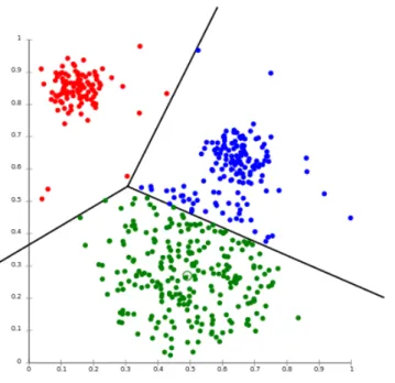
of is to find the properties of this probability density without the help of supervisor providing the correct answers [20, chapter 14, p. 486]. Clustering, self-organizing maps and principle component analysis are typical techniques used in unsupervised learning. Clustering partitions observations into groups (cluster), so that observa-tions in the same group are similar and observaobserva-tions in different groups tends to be dissimilar [20, chapter 14, p. 507]. Figure 2.2 shows an example of K-means clustering. K-means clustering requires the number of clusters k in advance. In this example, data was divided into three clusters which means k equals 3.

(10)

unsu-Figure 2.2: K-means Clustering fromhttps://en.wikipedia.org/wiki/Cluster_ analysis

pervised learning, which utilizes both labeled and unlabeled data. The motivation for semi-supervised learning is very practical: unlabeled data are cheaper and more plentiful to get than labeled data. It is easy to gain a great amount of unlabeled data in real world. For example, mountainous of images, documents and speech can be gained online. However, the prediction label for these data often requires human annotations and laboratory experiments [21]. One way to perform semi-supervised learning is called transductive learning. Using labeled data as training data and un-known data as test data, make predictions only for unlabeled data. Another method is called inductive learning, which is interested in predicting future test data [22].

2.2 Image Feature Extraction

Feature extraction transform the original data to a new dataset with a reduced number of variables. There are many reasons to perform feature extraction, for example reducing the size of input data, providing a relevant set of features for classification, and recovering new meaningful underlying variables to describe the data [23, chapter 10]. Feature extraction finds a transformation that lower the measurement dimension in order to gain a better understanding of data and improve classification performance. This transformation can be liner or non-linear and can be used in supervised or unsupervised learning .

(11)

CM Compact, robust Not enough to describe all colors, no spatial info

CCV Spatial info High dimension, high computation cost

Correlogram Spatial info Very high computation cost, sensitive to noise, rotation and scale DCD Compact, robust, perceptual meaning Need post-processing for spatial info

CSD Spatial info Sensitive to noise, rotation and scale

SCD Compact on need, scalability No spatial info, less accurate if compact

Texture is considered as an important feature for recognition and interpretation in human visual system. While color is usually a pixel property, texture can only be extracted from a group of pixels. Based on the domain where texture feature is ex-tracted, texture feature extraction methods can be divided into two main categories: spatial and spectral. For spatial text feature extraction method, pixel statistics or local pixel structures are computed and found in the original image domain. While spectral texture feature extraction method transforms an image into frequency do-main and then calculates features from the transformed image [26].

Figure 2.3: Shape Extraction by Subtraction and Thresholding [27]

Finding shapes in images belongs to high-level feature extraction. Many complex images can be decomposed into a set of simple shapes. For example, one approach for face recognition is to extract ears, eyes, nose and mouth such major facial shape features. Finding shape features including finding position, orientation and size of these components. Some simple feature extraction techniques are for example, thresholding, subtraction and template matching [27, chapter 5]. Figure 2.3 shows an example of shape extraction by subtraction and thresholding. Hough transform

(12)

is also a common technique for shape feature extraction in computer vision. Hough transform was first introduced to find lines and curves in images [28], but later it extends greatly and is used to locate positions of arbitrary shapes [29].

2.3 Neural Network

Artificial neural networks are computers simulating of biological networks of neuron in human brains. The earliest study in this field can be traced back to the 1940s. But due to limitations of the technology at that time, neural network was not so successful. Until the early 1980s, it caught the interests of researcher again. The central idea of neural network is to extract linear combinations of the inputs as derived features, and then model the target as a nonlinear function of these features [20].

Figure 2.4: unit neuron

Diagram of one neuron is presented in Figure 2.4. The variables x1, x2, x3 denote

inputs, while w1, w2, w3 are weights. The output is h(x), weighted sum of inputs

passed by activation function, as in the following equation

h(x) =g(w1x1+w2x2+w3x3) = g(WTx) (2.2)

where g is activation function, W =

   w1 w2 w3   and x=    x1 x2 x3   .

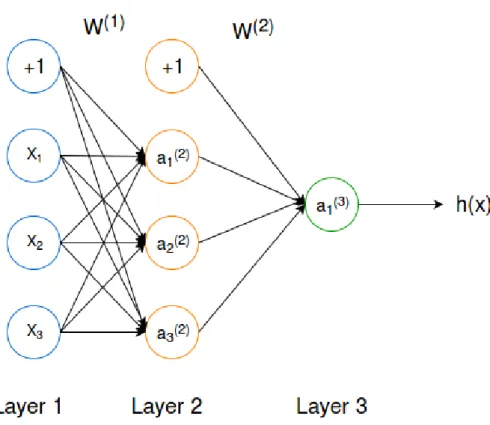
Neural networks are constructed by these neurons. A simple three-layer network structure is showed in Figure 2.5. Layer 1 and Layer 3 are input layer and output layer. Layer 2 is called hidden layer, a neural network can have many hidden layers in general. The equations of this three-layer network are given below:

a(j)=g(WTx) (2.3)

where a(_ij) is "activation" of unit i in layer j, and g represents is the activation function. The details of activation function will be discussed in subsection 2.3.1.

(13)

Figure 2.5: A Three-layer Neural Network

The output of this network is justa(3)_{, the activation at Layer 3. The input vector}

denotes as x and weight vector W(j) which maps from layer j to layer j+1. It is common to add bias units in neural network, such as the x0 and a

(2)

0 in Figure 2.5.

The initial weights of neural networks are usually chosen to be random values near zero. This model presented in Figure 2.5 is known as feed-forward neural network. Because there are no feed back connections which feed the outputs back to this network.

When design a neural network, how many layers the network should have, how layers connect to each other and how many units in each layer should all be taken in consideration. In the following subsections, we will talk about activation function, cost function and optimizer, which are very important concepts in neural network.

2.3.1 Activation Function

Activation can be considered as a switch in computational networks, which defines the output of a node given a set of inputs. It is also the key of transferring the learn-ing model from linear to non-linear. There are many common activation functions, such as Sigmoid, Tanh, rectified linear unit (ReLU) and softmax. AS we can see from Figure 2.6 and Figure 2.7, Tanh function converts a real value number into the range [-1,1], while sigmoid function maps the value into the range of [0,1]. Sigmoid function is used widely, which is also the predict function for binary logistic

(14)

regres-sion as mentioned in previous section. Equations of Tanh and Sigmoid functions are presented following: Tanh(x) = 2 1 +e−2x −1 (2.4) Sigmoid(x) = 1 1 +e−x (2.5)

From the equations we can see that Tanh is scaled version of Sigmoid, T anh(x) = 2Sigmoid(2x)−1.

Figure 2.6: Tanh Activation Function

Figure 2.7: Sigmoid Activation Function

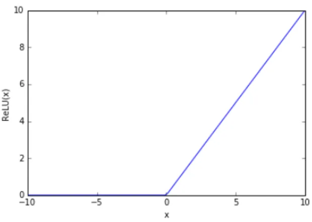
Figure 2.8 plots the activation function of ReLU. ReLU is the most popular activation function in deep neural network and Softmax is usually implemented as the last layer in neural network [30]. The equation of ReLU is shown below:

ReLU(x) = (

x if x >0

0 if x≤0 (2.6)

ReLU activation function has two advantages compared to Tanh and Sigmoid func-tions. First, it accelerates the convergence in stochastic gradient descent (we will

(15)

Figure 2.8: ReLU Activation Function

talk about stochastic gradient descent in next subsection 2.3.2). Second, it requires less operations compared to former two activation functions, which involves expo-nential computations. Softmax function is a generalization of Sigmoid function, it maps a K-dimensional vector of arbitrary real values into a a K-dimensional vector of values between 0 to 1.

2.3.2 Cost Function and Optimization

The cost function, also called loss function, or error function, is used to estimate parameters in statistics. Cost functions tell the difference between the predicted and real outputs. Common loss functions are mean squared error and logloss. The mean squared error loss function can be described as following equation,

J(θ) = 1 2m m X i=1 (ˆy(i)−y(i))2 (2.7)

whereyˆ(i) is estimated output, y(i) is real output ofith sample, and θis parameters vector of this learning model.

The logloss function, also known as binary cross-entropy, is often used in logistic regression problem. The logloss function equation is given below:

J(θ) =−1 m m X i=1 [y(i)loghθ(x(i)) + (1−y(i)) log(1−hθ(x(i)))] (2.8)

wherehθ(x)is the prediction rule,x(i)isith input,y(i)is is real output ofith sample.

Fitting a neural network is trying to find the model that fits the training data well. Optimizer finds best parameters when J(θ) value archives local minimal. A most common optimization method in large scale machine learning is called stochastic gradient descent [31]. The concept of gradient descent method is updating

(16)

param-eters in the opposite direction of gradient of cost function, ∇J(θ). The value of J(θ)decreases fastest in the direction of negative ∇J(θ). There are three kinds of gradient descent methods: batch gradient descent, stochastic gradient descent and mini-batch gradient descent.

In batch gradient descent, for each updating, the gradient of cost function with regard to θ is on the whole training data set. Take the logloss cost function for example. The equation of parameter updating is presented as following equations,

θ=θ−α ∂ ∂θJ(θ) (2.9) ∂ ∂θJ(θ) = 1 m m X i=1 (hθ(x(i))−y(i))x(i) (2.10)

where x(i) _{is the input of} _{ith sample and} _α _{is learning rate. Learning rate decides}

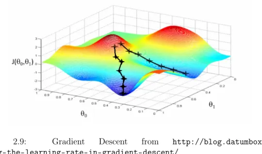
the step size of updating parameters. If the learning rate is too large, it is likely to miss the valley value of J(θ). Keep iterating θ using the Equation 2.9 until J(θ) converges to the local minimum. Figure 2.9 shows gradient descent with two parameters θ0 and θ1. The initial values of parameters will decide the descent path

and the final value ofJ(θ). As we can see from Figure 2.9, two different start values of θ0 and θ1 end up with two different paths and local minimum J(θ0, θ1) values. If

the training set is large, then the calculation of gradient descent is very slow. Thus, this method is not so commonly used in practice.

Figure 2.9: Gradient Descent from http://blog.datumbox.com/

tuning-the-learning-rate-in-gradient-descent/

Stochastic gradient descent (SGD) updates parameters taking one training exam-ple per time and updates repeatedly. Therefore, SGD is faster than batch gradient descent. The equation of SGD is presented in Equation 2.11.

(17)

tum was introduced to help accelerate SGD in the relative direction and reduces oscillations [32]. A comparison of SGD with and without momentum is presented in Figure 2.10. Momentum adding a fractionγ of the last step update vector to the current update vector as in the following equations:

Vt=γVt−1+α∇J(θ) (2.13)

θ =θ− Vt (2.14)

where V is the parameter update vector, initialized as α∇J(θ), α is the learning rate and the momentum parameterγ is usually set to 0.9.

(a)

(b)

Figure 2.10: (a) SGD Without Momentum (b) SGD With Momentum from http:

//sebastianruder.com/optimizing-gradient-descent

Nesterov accelerated gradient (NAG) [33] updates the weight vector based on the previous vector and the gradient at the approximate future position of parameters

(18)

according to the below equations:

Vt =γVt−1+α∇J(θ−γVt−1) (2.15)

θ =θ−Vt (2.16)

We know that we use momentumγVt−1 to compute the parameters, thusθ−γVt−1

gives us an approximation of the next parameters position. NAG is applied in SGD to help to speed up convergence, more details about NAG can be found in [34].

2.3.3 Backpropagation

In the beginning of this section, we talked about how to compute the output of neural network. This process is also called forward propagation. Backpropagation trains the network from last layer to first layer backwards. The goal of backpropagation is also minimizing cost function J(θ), just like what optimizer does in the last subsection. An illustration of back propagation is presented in Figure 2.11.

Figure 2.11: Back Propagation

The first step of backpropagation is feed forward propagation, just like normal neural network as we mentioned in the beginning of this section. Feed the input to neural network and compute the output for each node and store the values. Then back propagates the output activations to the neural network to compute the error for each node, which is marked as δ in the Figure 2.11, where δ_j(l) is the error for jth node in layer l. Recall that a(_jl) is the activation (output) for jth node in layer l. The error for the output layer can be computed with:

δ(L) =y−a(L) (2.17)

(19)

∂J(θ) ∂θ_i,j(l) =a (l) j δ (l+1) i (2.19)

We update the weight θ(_i,jl) by subtracting it with αa_j(l)δ(_il+1), like what SGD does, whereα is the learning rate.

Because the desired outputs of the data is required in backpropagation algorithm, so backpropagation is usually considered as a supervised learning method. From the analysis above, we can see that why this algorithm is called back propagation. Because the error values are counted from the last layer to the first layer backwards. Backpropagation is a vital and yet not an easily understood algorithm in neural network. Although we do not apply this algorithm in our thesis, backpropagation is widely used in artificial neural network. Backpropagation through time (BPTT) [35], a type of backpropagation algorithm, is usually used to train recurrent neural networks (RNN).

2.4 Deep Learning

The traditional machine learning system is limited in processing natural data with their raw form, such as speech, image and music. Therefore, for a long time machine learning requires expensive human labor and expertise to extract useful features from raw data. Representation learning or feature learning is a set of methods that can automatically find representations from raw data for classification or detection [36]. Deep learning is belonged to representation learning with many layers of represen-tations, that each layer transform the representation (starting from the raw input data) into a representation at a higher, slightly more abstract level [37]. It has been proven that deep learning methods can find intricate structures inside large amount of data and represented it with multiple levels of features. Deep learn-ing has archived many breakthroughs in the field of large-scale image classification [9; 10], object detection [38] and semantic segmentation [39; 40]. Two very popu-lar models in deep learning recently are convolutional neural network and recurrent

(20)

neural network [37]. Convolutional neural network is the key point of our paper, we will discuss it in Subsection 2.4.1

2.4.1 Convolutional Neural Network

Figure 2.12: Fully Convolutional Network for Content Based Image Retrieval

Figure 2.13: Fully Convolutional Network for Semantic Segmentation

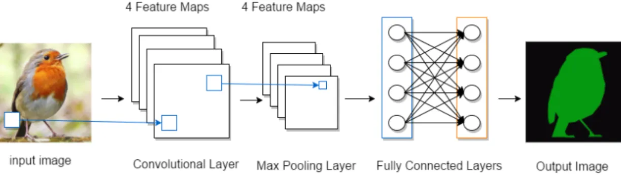
Convolutional neural network is designed to handle data that comes in the form of multiple arrays [37], for example of color images that has R, G, B three channels of 2D arrays. A typical use of CNN is for classification, where the output is a single class label, as in Figure 2.12. Input an image, the output predict the class of the image content, either its a bird or a car etc. Therefore CNN can be used for image retrieval. CNN can be also used for segmentation tasks, where the output is also an image that contain location information. In other words, a class label is assigned to every pixel in the output image. For example, in Figure 2.13, given a bird image as input, the output is also an image, where pixels belong to bird is colored with green and other pixels are marked as black. The first few stages of a typical CNN are composed of convolutional layers, ReLU layers and max pooling layers. Convolutional layers produce a set of linear combinations of inputs, as a form of feature map. Then the feature map pass through the ReLU non-linear activation function layer. Max pooling layer aggregates the information from ReLU layer and produces a feature map with smaller spatial size. A fully convolutional network

(21)

Figure 2.14: An example of 2D convolution [30]

The first layer is input image, with sizeh×wwith a depth of 3. handware height and width, belonging to spatial dimensions. The convolutional layer is composed of four feature maps, while each feature map is connected to the local region of the image in a spatial extend. The connection is fully along the depth axis. For example, if we apply a convolution kernel of size3×3, and the image has a depth of 3. Then each neuron of the feature map in the current layer has a3×3×3connections with the previous layer. Comparing with fully connected layers, convolutional layers reduce the parameters amount greatly. Figure 2.14 is an example of 2D convolution. In this figure the convolutional kernel size is 2×2, the kernel is also called receptive field or patch in some paper. The variables w, x, y, z represent kernel weights. The input is a4×3 image, where variables a, b, ..., l represent pixel values. The output is a3×2image, whose pixel values are indicated inside each box. The kernel moves inside the input image one pixel per time, which is stride 1. In this figure, we only output the position where the kernel is entirely inside the image, this is called valid convolution. But sometimes zero-padding will be needed if the remainder of image

(22)

size divided by filter size is not equal to zero. Zero-padding is padding the input image with value of zeros around the border. With zero-padding, we can control the output size of convolution.

The k-th feature map is denoted ashk and the weights areWk. The same feature map share the same weight. The parameters sharing scheme is applied under one reasonable assumption that the feature we learn at one spatial position should also be useful to other positions of the image. Parameters sharing reduces the parameters . The variablexij denotes the data vector of the input image at the coordinate(i, j).

Then the feature map can be obtained with

hk_ij =ReLU((Wk∗x)ij +bk) (2.20)

where ReLU is a non-linear activation function and∗represents convolution manip-ulation,bk is the bias.

Figure 2.15: Max Pooling

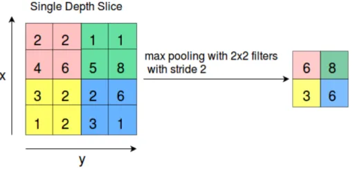
Usually the convolutional layer is followed by a ReLU non-linear layer and a max pooling layer. ReLU layer introduces the non-linearity into CNN. The role of pooling layer is to reduce the spatial size of feature maps to reduce the number of parameters and also control overfitting consequently. Max pooling decreases the computation work and increases the position invariance at the same time. The size of max pooling is usually 2×2, which means down sampling the feature map by 2. After max pooling, the depth dimension remains unchanged. Figure 2.4.1 shows an example of max pooling. The input is a single depth slice of size 8×8. The filter size is2×2, which outputs the maximum of value in the2×2input neighborhood.

2.4.2 Overfitting

A learning algorithm is used to predict unknown data after trained by training data. In training phase, model is trained by maximize the performance on train

(23)

Figure 2.16: Overfitting in Supervised Learning fromhttps://en.wikipedia.org/ wiki/Overfitting

data. However, the efficacy is measured by its ability to predict the unknown test data. When the model is excessively complex and the train data is rare, overfitting is likely to occur. Because the model begins to memorize the training data rather than learning the trend. When the training error is raising, but the validation error decreases, overfitting may have already occurred, as shown in Figure 2.16.

Cross-validation is often used for preventing overfitting in machine learning. The idea behind cross-validation is simple. One of cross-validation method is called k-fold cross-validation. The original sample is divided into k sub-samples of equal size. One of the sub-sample is used as validation data and the other k-1 sub-samples as train data. The cross-validation process is repeated for k times, with each sub-sample is used exactly once as validation data. The measured performance of k-fold cross validation is the average of computed values in the k loop. The goal of cross-validation is to measure how the model fit the data independent of the data used to train.

Deep learning models with a large amount of parameters are very powerful to learning intricate relationships inside data. However, with limited number of train-ing data, many of learned relationships will be result of sampltrain-ing noise. This leads to overfitting. Dropout is a regularization technique that used to prevent overfitting in neural networks [41]. The key idea of dropout is dropping out units from a neu-ral network. Dropping out a unit means removing it from the network temponeu-rally, along with its all incoming and outgoing units. The choice of dropping out which units is random. Each unit has a fixed probability to retain independent of other units. Figure 2.17 shows how drop out works in training and test phases. During each training, the original neural network is sampled to a new neural network. At test time, no dropout is applied, but the weights are scaled down. It has proven

(24)

(a) At Training Time

(b) At Test Time

Figure 2.17: Dropout. (a): A unit at training time that is present with probability p and is connected to units in the next layer with weights w. (b): At test time, the unit is always present and the weights are multiplied by p. The output at test time is same as the expected output at training time. [41]

that dropout technique can reduce overfitting significantly. Plus, applying dropout in neural networks improves the performance in general for a wide range of applica-tions such as computer vision, speech recognition and documents classification.

2.5 Semantic Segmentation

Humans can recognize the visual world easily. However, it is much more difficult for machines to interpret a image or a video. The goal of computer vision is making useful decisions of real physical objects and scenes based on images [8]. Object recognition, detection and segmentation are front areas in computer vision over the last two decades. Object detection finds bounding box of semantic objects inside a digital image. For example, Figure 2.18 is an example of object detection from Large Scale Visual Recognition Challenge 2014 [42]. Detecting face location [43] and face recognition [44] are the most popular applications of object detection. It is natural that progress from coarse detection to a fine prediction at every pixel, which is semantic segmentation.

The term of semantic segmentation refers to partition an image into different regions based on the semantic meaning of objects in the image at a pixel level. The input of semantic segmentation is an image and the output is also an image, where

(25)

Figure 2.18: Object Detection [42]

Figure 2.19: Semantic Segmentation [13]

each pixel of the image is labeled based on its semantic. For example, in Figure 2.19, the input image is a man riding on a horse. In the output image, the man is colored with pick and the horse shape is filled with magenta while the background is black. Traditional segmentation methods utilize region and parts information [45]. Alternative region-based approaches such as conditional random fields, refining top-down detection, scoring bottom-up region hypothesis.

With the development of deep learning, neural networks are used for semantic segmentation lately. CNN and RNN are state-of-art frameworks for this task. Many previous approaches have used CNN for semantic segmentation [40; 46; 47]. The first work to train FCN end to end for pixel-wise prediction and from supervised pre-training is [13]. However, most of the state-of-art semantic segmentation are based

(26)

on natural scenes. As far as we know, this thesis is the first work that perform semantic segmentation on human faces particularly.

2.6 Evaluation metrics

Model performance assessment is an important aspect in machine learning. To select the best performing algorithm, scientists usually apply evaluation metrics to rank the candidate algorithms. The most common semantic segmentation measurement is pixel-wise classification accuracy. There a a few evaluation metrics for pixel-level accuracy, such as pixel accuracy, mean accuracy and mean intersection over union. Let k ∈ _N be the number of classes, and nij with i, j ∈ 1, ..., k be the number of

pixels of class i which are predicted to belong to class j. (nij) is called a confusion

matrix. Let ti = P_j(nij) be the total number of pixels of class i. Pixel accuracy

measures the proportion of correctly labeled pixels: P

inii

P

iti . Mean accuracy measures

the proportion of correctly labeled pixels for each class and then averages it: 1_kP

i nii

ti .

Figure 2.20: Intersection and Union of Sets A and B

Here we focus on the mean intersection over union. This measurement is also called Jaccard index. Jaccard index is used for comparing similarity and diversity between sets. In our thesis, Jaccard will be used to measure the coincidence fraction of the face image actual location and prediction location. Thus we can assess the accuracy of segmentation in consequence. Figure 2.20 shows two sets A and B as well as their intersection and union. The Jaccard index calculation formula is given below: J ac(A, B) = |A T B| |AS B| (2.21)

If A and B are empty sets, we define J ac(A, B) = 1. The value of Jaccard index is between 0 and 1, the higher value meaning higher similarity between two sets.

(27)

In our experiment, we have two image databases, background images and faces images. The background images are pictures of random scenes in the campus of Tampere University of Technology, while face images are faces of students or staff from this university. Examples of background image and face image are shown in Figure 3.1 and Figure 3.2. To generate the training and test image database, we have to process these two original image database.

(28)

Figure 3.2: Face Image Example

Figure 3.3: Dataset Image Example

Step 1: crop and resize random selected background and face image. First, we crop the background image into a equal width and height image at a randomly chosen location, whose size is sampled from uniform distribution with low bound of 512 and high bound of 1024. Then resize the cropped background image to 512×512. Second, we crop the face image from 0.2×width to 0.8×width, and 0.2∼0.8×height because the human face is located in this area of face image. After cropping, the new face image size multiples by 0.7.

Step 2: add the face to background image. On the background image, randomly choose an area with the same size of face image and compute the stand deviation of its red channel. Repeating the step for 10 times, record the standard deviation

(29)

whereµis expectation andσis standard deviation of Gaussian distribution (normal distribution), whose figure is shown in Figure 3.4. When µ = 0 and σ = 1, it is called standard normal distribution. The equation of 2D Gaussian filter is shown following: G(x, y) = 1 σ√2 2πe −x2+y2 2σ2 _(3.2)

with x and y represent horizontal and vertical directions.

(a) Gaussian Distribution

(b) 2D Gaussian Distribution

Figure 3.4: Gaussian curves from https://en.wikipedia.org/wiki/Gaussian_

function

The figure of 2D Gaussian is shown in Figure 3.4. Applying a 2D Gaussian filter to an image is convolving the image with 2D Gaussian function. In theory, Gaussian

(30)

distribution is non-zero everywhere, which will require a infinitely large convolution kernel. Thus in practice, the influence of points greater that 3σ distance from the mean is removed. "Gaussian averaging operator has been considered to be optimal for image smoothing" [27, p. 88].

Iterating these two steps for 50000 times, keep all the face locations information in a text file for later use. Therefore, we gain a dataset consisting of 50000512×512

RGB images together with information of face location information in each. An ex-ample of generated image is shown in Figure 3.3. Figure 3.5 gives an straightforward look of the text file.There are many sections in this text file. In each section, the first row is the image name and the second row stores the image location. While the following rows indicate the face location in the image, while ulc:upper left col-umn; ulr: upper left row; lrc: lower right colcol-umn; lrr: lower right row. Figure 3.6 illustrates the face location indicators in a visual way.

Figure 3.5: Screen shot of Image Information File

Figure 3.6: Illustration of Face Location Information. The blue rectangle represents the image, and the red square is face area.

(31)

Figure 3.7: Our CNN Architecture. At the bottom of feature maps, their sizes are provided. A Conv Block consists of a convolutional layer, a ReLu non-linear layer and a max pooling layer.

In the thesis, we apply two different network architectures, our own CNN archi-tecture and U-net [48]. Our own CNN archiarchi-tecture is shown in Figure 3.7. For space reason, we only represent one convolutional layer version in this figure. As we see from the Figure 3.7, the input image will pass through threeConv blocks. A

Conv block is a combination of convolutional layers, a ReLU non-linear layer and a max pooling layer. The number of theConv blocks will affect the output image size, which is decided by the number of max pooling layers. Recall the main function of max pooling layer is down sampling, as we discussed in subsection 2.4.1. An illustra-tion of the relaillustra-tionship between the number ofConv block and size of output image is shown in Table 3.1. With the increasing of Conv blocks from 1 to 4, the size of output image is decreasing from128×128 to16×16. The number of convolutional layers in each Conv block can be changed also. Figure 3.8 shows Conv blocks with number of convolutional layers ranging from 1 to 3. A few convolutional layers stack in the beginning of Conv block, then followed with a ReLU non-linear layer and a max pooling layer. The sequence of ReLU and max pooling layer can be switched, which does not affect the architecture. However, it is a usual practice to put ReLu layer in front of max pooling layer.

In the first Conv block, we apply a drop out layer after convolutional layers to prevent over fitting. Due to space reason, we did not plot out the drop out layer in Figure 3.7. All convolution kernels have the same size of 3×3, which is the smallest size to capture the information from left&right, up&down, center. Zero-padding is

(32)

Number of Conv Block Size of Output Image

1 128×128

2 64×64

3 32×32

4 16×16

Table 3.1: Relationship between number of Conv Block and size of output image

Figure 3.8: Conv Blocks with Different Number of Convolutional Layers applied in all convolutional layers to keep the spatial size. Max pooling is performed over a 2×2 filter window, with stride 2. The output layer is also a 2D convolutional layer, with 1 output filter, followed by a sigmoid activation function. Thus the output variables only have two classes, where pixel belongs to face is labeled as 1, and pixel belongs to background is labeled as 0. Figure 3.9 shows an example of output image.

The second network architecture is called U-net [48]. The U-net architecture is showed in Figure 3.10. U-net consists of a contracting and an expansive path, where the expansive path is symmetric to the contracting path, yield a u-shape architecture. The input and output image have same spatial size. The contracting

path repeatedly apply two 3×3 convolutional layers, each followed with a ReLU

(33)

Figure 3.9: An Example of Output Image

sampling, the number of feature maps is doubled in the next level convolution. In the expansive path, each convolutional layer is followed with a ReLU layer and two convolutional layers is followed with a upsampling layer. The number of feature maps is halved after upsampling. Different from the U-net in [48], in this thesis we do not copy the corresponding cropped feature map from contracting path. The last layer is a 3x3 convolutional layer, with a Sigmoid activation unit. The output has only one channel, which means the output is a black and white image as former experiments.

Our CNN architecture applies a typical CNN structure. U-net has contracting path with down sampling layers and expansive path with upsampling layers. The obvious and biggest difference between our CNN and U-net is that our CNN does not have the expansive path. Adding expansive path does not only increase convolutional layers but also scale up the output image size. Another great difference is that U-net have much more feature maps than our CNN, which allow U-net to propagate richer context information to higher resolution layers.

(34)

Figure 3.10: U-net Architecture. Each blue box represents a multi-channel feature map. The number of feature channels is located at the top of the box. The spatial size of feature map is denoted at the lower left of the box.

(35)

Our experiments are performed using Python, Theano and Keras. Theano is a Python Library that allows users to define, optimize, and evaluate mathematical expressions involving multi-dimensional arrays efficiently [18]. A new technical re-port of Theano is [49]. "Keras is a minimalist, highly modular neural networks library, written in Python and capable of running on top of either TensorFlow or Theano" [17]. All the experiments are running on the Merope, the Linux-based clus-ter for parallel computing for tampere cenclus-ter for scientific computing with NVidia Tesla K40 and Tesla M2090 GPU’s.

The rest of this section will describe the details of our experiments. Subsection 4.1.1 will show how we prepare our data and pre-process them before we imple-menting deep learning. Subsection 4.1.2 will explain parameters we set for training networks. Last but not least, subsection 4.1.3 will discuss how and why we set all the experiments.

4.1.1 Image Preparation and Preprocessing

In image collection phase, we randomly choose a large amount of images from the database, which the total number is set by ourselves. 10% of selected images are used for testing and others for training. Recall that sizes of images from the database is512×512. Before we do image pre-processing, we first resize all the image sizes to

256×256. We perform image pre-processing by scaling all the image pixels to [0,1]. The range of pixel values for RGB image is [0,255]. We first subtract all the pixels values with minimum pixel value, then divide them by the maximum pixel value. The image pre-processing we do is called simple scaling in data normalization. This is useful for later processing since many parameters assume the data has already been scaled in reasonable range. Such data and image pre-processing is always needed in deep learning networks, We generate the true output images for training and test in this image collection phase also. The size of true output images is determined by the actual experiment. In the output images, face area pixels are labeled by 1 and pixels belong to background are labeled by 0.

(36)

4.1.2 Train

In subsection 2.3.2, we talked about mini-batch SGD, momentum and Nesterov accelerated gradient. We trained both networks by SGD with momentum, with a mini batch size of 16 images. The SGD used in Keras is actually mini-batch SGD. Training with a batch size of 16 meaning that propagate 16 image samples to train the network each time. An epoch is completed when every training image has already been fed into the network once. We use momentum of 0.9 and apply Nesterov momentum. We first set the training with 100 epochs and the learning rate to 0.001. However, after a few tests of the network, we realize that the accuracy still has the trend of growing at the end of 100 epochs. Thus, we decide to improve the epoch number to 200 and decrease the learning rate to 0.0008. The learning rate decay is 10−6. In practice, it is helpful to to renew the learning rate over time. The learning rate decay applies a slightly decay of learning rate over each update which prevents the learning rate from too high. The loss function is binary cross-entropy, which is logloss cost function as we mentioned in subsection 2.3.2.

4.1.3 Experiment Settings

There are four main experiments in this thesis, where the basic network architecture is our CNN in the first three experiments and U-net architecture is only used in the last experiment. In the first experiment, we want to test the effect of image number

to accuracy. Therefore, we fix the Conv Block number as 3 and 3 convolutional

layers in each block. Then we validate the network with image number of 5000, 10000, 15000, 20000 separately. The learning performance is indicated by Jaccard index.

In the second experiment, we want to test how the number convolutional layers affect the performance. In this experiment, we use 3Conv Blocks in total, the same as first experiment. However, this time we change the number of convolutional layers in the block. First, we only put 1 convolutional layer in each Conv Block. Then for the following settings, we increase the number of convolutional layer by 1 each time. The total training and test image number is fixed as 15000 during the whole second experiment. The learning performance is still indicated by Jaccard index. However, we add one more indication which is total parameters number in this experiment.

For the third experiment, we are interested in how our CNN architecture predict output images with various sizes. We have three different output image sizes in this experiment: 64×64,32×32and16×16. In order to alter the size of output image,

we must change the number of Conv Blocks correspondingly. For image output of

size 64× 64, the number of Conv Blocks is 2. Conv Blocks number of 3 and 4

(37)

4.2 Results

This section presents all the results of our thesis based on all the four experiments

described in the previous section. For the first experiment, we fix the network

architecture and alter the train&test total image number. The input image size is

256×256, and the size of output image is 32×32. The results of this experiment are given in Table 4.1, where we measure the network performance using Jaccard

Index. The Conv/block means the convolutional layers number in eachConv Block,

which is 3 in the first experiment. And there are 3Conv Blocks in total. When train and test out CNN with 5000 images, the Jaccard Index is 70.68%. After increasing the total image number from 5000 to 10000, the accuracy increases 12.66%. While the accuracy increase 3.41%, after image number increasing from 10000 to 15000. The performance increases even less, 1.25%, when image number increase to 20000. We can see that with the increasing of image number, the Jaccard index increases, which indicates a better performance. In other words, adding training images has a positive effect in convolutional neural network, which results a more accurate prediction. When the training images number is not large enough, adding images number will improve the performance rapidly. However, when the training images are already very large, increasing images will not improve performance so much.

Image Number Jaccard Index

5000 70.68%

10000 83.34%

15000 86.75%

20000 88.00%

Table 4.1: Conv Layers/block: 3, Conv Block: 3

In the second experiment, we would like to dig dipper on the convolutional neural network architecture. More precisely, we want to know how the depth of CNN affect the prediction accuracy. Therefore, we fix the training and test image number as 15000, and steadily increase the number of convolutional layers in eachConv Block.

(38)

The input image size is 256×256, and the size of output image is 32×32. The results of this experiment is presented in Table 4.2. The accuracy is still represented by Jaccard Index, but we add another two columns,total parameters number and total convolutional layer number, which indicate the complexity of neural network.

The number of Conv Blocks is fixed as 3. When there is only one convolutional

layer in each Conv Block, the total convolutional layers number is 5 including the 2 convolutional layers in the last stage. Increasing one convolutional layer for each

Conv Block will increase the total convolutional layers by 3. As a consequence, the total parameters number will increase by 27744. With the number of convolutional

layers in each Conv Block increasing, the accuracy also increases. However, the

magnitude of increment is descending, from the first 6.79% increment to 4.06% then to the final 1.00%. In conclusion, with the increasing of convolutional layers, the CNN gain a better prediction performance. This is not hard to understand that with more convolutional layers the network has a larger number features to learn images. But when the depth of network increased, the network also become more complex to train. Too many parameters will cause overfitting and troubles in finding local minimum. Thus the prediction accuracy will not rise linearly with the increasing of layers number.

Conv Layers/block Total Parameters Total Conv Layers Jaccard Index

1 28929 5 75.90%

2 56673 8 82.69%

3 84417 11 86.75%

4 112161 14 87.75%

Table 4.2: Image Number: 15000, Conv block: 3

Number of Conv Block Output Image Size Total Conv Layers Jaccard Index

2 64×64 8 71.68%

3 32×32 11 86.75%

4 16×16 14 88.36%

Table 4.3: Conv Layers/block: 3, Image Number: 15000

In the third experiment, we want to test how our CNN prediction result differs with distinct size of output image. The output image size we choose are 64×64,

32×32 and 16×16, while the size of input image is all the same, 256×256. Table 4.3 shows the results for our third experiment. From the list we realize that the network achieves a best accuracy when the output image size is16×16. One reason is that there are more convolutional layers for this output compared the other two. The other reason is that there are less pixels needed to be classified for the output

(39)

Conv Blocks has more max pooling layers. Because max pooling layer will aggregate the statics of features from various locations to get better features for classification. Figure 4.2 compares an example of real output image and predicted output image. We can see that the prediction result is quite good. An example of Jaccard Index Evolution is shown in Figure 4.3(a). In this figure, the accuracy rises slowly before 10 epochs. Between 10 to 50 epochs, Jaccard Index increases sharply. After running for 50 epochs, the Jaccard index floats in a tiny scope and rises slowly. Finally the value of Jaccard index trends to stay stable after 200 epochs. During our experiment, sometimes Jaccard index goes wrong like in Figure 4.3(b). Before 30 epochs, the Jaccard Index fluctuates dramatically. However, after 30 epochs, Jaccard index drops to 0 suddenly and is never able to come up again. One possible reason for this situation is that learning rate is set too high, SGD misses the local minimum value and goes further. An example of our validation loss curve is shown in Figure 4.4. The loss drops from 0.18 to 0.14 very fast at the first epoch, then successively decreases in the following epochs. This means our network is learning form the database and the optimizer is working well. Recall the goal of optimizer is minimizing the loss. The final loss is 0.024.

From the results of the first three experiments, we can draw a conclusion that our CNN architecture is suitable and accurate for human face semantic segmenta-tion. In addition, increasing image number and convolutional layers will improve the segmentation accuracy. However, after the image number is saturated and the convolutional neural network gets complex enough, adding image number and con-volutional layers will not continue increasing the accuracy. Besides, the output size of CNN affects the accuracy also. A smaller size of output image receives the best segmentation accuracy comparing with other bigger size outputs. This is because the neural network has less points to predict and more convolutional layers with a smaller output size. As far as our knowledge, there are no articles using our same database or network architecture. Thus, it is not possible to compare our results with the state-of-art work in semantic segmentation. However, this can be the future working direction that apply other deep learning architecture with our database, for

(40)

(a) output image size: 64x64

(b) output image size: 32x32

(c) output image size: 16x16

(41)

(a) True Output Image

(b) Predicted Output Image

Figure 4.2: A Comparison of True Output Image and Predicted Output Image. In the last experiment, we validate the U-net network with 15000 images includ-ing traininclud-ing and test images. The structure of U-net is plotted and explained in section 3.2. The input and output size share the same spatial size 256×256. The validation accuracy for U-net is 90.70% measured by Jaccard index. We compare the result of U-net with our CNN architecture in Table 4.4. The training and test

image number for our CNN is also 15000. Our CNN is a CNN with 4Conv Blocks

and 4 convolutional layers in eachConv Block and 18 convolutional layers in total, including the 2 convolutional layers in the last stage. The input size is 256×256

(42)

(a) A Normal Jaccard Index Evolution Curve

(b) When Evolution of Jaccard Index Went Wrong

Figure 4.3: Evolution of Jaccard Index

and the output size is 16×16. The accuracy for our CNN is 88.99%, slightly worse than the result of U-net. U-net model achieves a better performance than all the experiments using the first CNN architecture. However, U-net is much more slow to train due to its complexity. The former experiments all take around one day to train, while U-net takes approximately 8 days. Considering the accuracy and speed, we can make an conclusion that our CNN is better than U-net for the task of human face semantic segmentation.

Network Conv Layers Total Parameters Output Image Size Accuracy Training time our CNN 18 149153 16×16 88.99% ≈1 day

U-net 18 28209089 256×256 90.70% ≈8days

Table 4.4: Comparison of U-net and our CNN

To understand how our convolutional neural networks learn the images we feed them, we visualize the outputs of convolutional layers (after ReLU activation) and

(43)

Figure 4.4: Evolution of Validation Loss Example

first layer weights. Figure 4.5 shows the outputs of all convolutional layers of our CNN architecture with 2Conv Blocks and 2 convolutional layers in each block. The input image is Figure 3.3. Each convolutional layer has 32 feature maps. Every box corresponds to a feature map in that layer. We can see that many of the activations in feature maps are black, which means their values are zero. In the last convolutional layer which is also the output layer, the face area is activated as we can see the white square are in the output. Unfortunately, there are some areas are wrong activated in the output also. If we feed the same input image to the CNN architecture with 3 Conv Blocks and 3 convolutional layers in each block, the mistaken activated area disappear as shown in Figure 4.6. The first convolutional

layer weights are plotted in Figure 4.7. Each box denotes a 3×3 convolutional

kernel. In each convolutional kernel, lighter color indicates a smaller weight value and darker color indicates a larger weight value. Usually we only visualize weights of the first layer which deals with the raw image pixel data. But it is also possible to see weights of deeper layers.

(44)

(45)

Figure 4.6: Last Convolutional Layer Output of our CNN with 3Conv Blocks and 3 convolutional layers in each block.

(46)

5. CONCLUSIONS

This thesis is inspired by [13], which is known as the first work to train fully convo-lutional network for end-to-end and pixel-wise supervised training. This article has proven that fully convolutional networks can achieve the state-of-art segmentation for a wide range of objects. Our thesis explores the question that does convolutional neural network serves a good segmentation for human faces.

Our thesis applies two CNN structures, one is proposed by ourselves, the other is U-net. Both network architectures achieve good accuracies, our CNN gains accuracy up limited to 88.99%, while the U-net receives accuracy of 90.70%. The U-net performances slightly better than our proposed CNN. However, our CNN takes approximately one eighth time of U-net for training and test. Therefore, we can draw a conclusion that convolutional neural networks are accurate and suitable for human faces semantic segmentation. Besides, our CNN architecture is better than U-net considering factors of accuracy and speed.

After we confirming that convolutional neural network is efficient for human faces segmentation task, we would like to improve the performance. More precisely, we would like to investigate the factors that affect the validation accuracy. We proposed three most possible factors: the number of training and test images, the depth of network and the output image size.

We fix our CNN structure with 3Conv Blocks and 3 convolutional layers in each block, while changing the total train&test image numbers from 5000 to 20000, with increment of 5000 images per time. The accuracy for 5000 images is 70.68%; for 10000 images is 83.34%; for 15000 images is 86.75%; for 20000 images is 88.00%. Increasing the image number from 5000 to 10000, the accuracy improves significantly. However, when image number is already large enough, adding images only increase the accuracy slightly.

In order to discover how the depth of CNN affects the accuracy, we apply a CNN architecture with 3Conv Blocks and increasing the convolutional layers number per

block from 1 to 4. The CNN with one convolutional layer in each Conv Block gets

the lowest accuracy, 75.90%. While the CNN with 4 convolutional layers in each

Conv Block gets the highest accuracy, 87.75%. In conclusion, increasing the depth of CNN will increase the accuracy. But this increment is not unlimited. As the CNN gets more complex, adding layers has a more micro improvement of the accuracy.

(47)

Deep convolutional networks are often applied in the field of large-scale image classification, object detection and semantic segmentation. Our thesis has proven that convolutional neural network is also efficient, accurate and suitable for human faces segmentation. Besides, adding training and test image number, convolutional layers and decreasing the size of output image are all beneficial for the segmentation accuracy. However, because of the uniqueness of our database and convolutional neural network architecture, it is not possible to compare our results with the state-of-art segmentation. This could be our future research direction, that apply pre-trained CNN models on our database.

(48)

REFERENCES

[1] Bruce G Buchanan. A (very) brief history of artificial intelligence. Ai Magazine, 26(4):53, 2005.

[2] James H Martin and Daniel Jurafsky. Speech and language processing.

Inter-national Edition, 710, 2000.

[3] Igor Kononenko. Machine learning for medical diagnosis: history, state of the art and perspective. Artificial Intelligence in medicine, 23(1):89–109, 2001. [4] Nicu Sebe. Machine learning in computer vision, volume 29. Springer Science

& Business Media, 2005.

[5] Christopher M. Brown Dana H. Ballard. Computer Vision. Prentice Hall, 1982. [6] Paul Viola and Michael Jones. Rapid object detection using a boosted cascade

of simple features. In Computer Vision and Pattern Recognition, 2001. CVPR

2001. Proceedings of the 2001 IEEE Computer Society Conference on, volume 1, pages I–511. IEEE, 2001.

[7] Navneet Dalal and Bill Triggs. Histograms of oriented gradients for human

detection. In 2005 IEEE Computer Society Conference on Computer Vision

and Pattern Recognition (CVPR’05), volume 1, pages 886–893. IEEE, 2005.

[8] Linda Shapiro and George C Stockman. Computer vision. 2001. ed: Prentice

Hall, 2001.

[9] Alex Krizhevsky, Ilya Sutskever, and Geoffrey E Hinton. Imagenet classification

with deep convolutional neural networks. In Advances in neural information

processing systems, pages 1097–1105, 2012.

[10] Karen Simonyan and Andrew Zisserman. Very deep convolutional networks for large-scale image recognition. arXiv preprint arXiv:1409.1556, 2014.

[11] Kaiming He, Xiangyu Zhang, Shaoqing Ren, and Jian Sun. Deep residual learning for image recognition. arXiv preprint arXiv:1512.03385, 2015.

[12] Liang-Chieh Chen, George Papandreou, Iasonas Kokkinos, Kevin Murphy, and Alan L Yuille. Semantic image segmentation with deep convolutional nets and fully connected crfs. arXiv preprint arXiv:1412.7062, 2014.

[13] Jonathan Long, Evan Shelhamer, and Trevor Darrell. Fully convolutional

net-works for semantic segmentation. In Proceedings of the IEEE Conference on

(49)

2016.

[16] Marta R Cojussà and Carlos Escolano. Morphology generation for

sta-tistical machine translation using deep learning techniques. arXiv preprint

arXiv:1610.02209, 2016.

[17] François Chollet. Keras. https://github.com/fchollet/keras, 2015.

[18] Theano Development Team. Theano: A Python framework for fast computation of mathematical expressions. arXiv e-prints, abs/1605.02688, May 2016. [19] Jaime G Carbonell, Ryszard S Michalski, and Tom M Mitchell. An overview

of machine learning. In Machine learning, pages 3–23. Springer, 1983.

[20] Jerome Friedman, Trevor Hastie, and Robert Tibshirani. The elements of

sta-tistical learning, volume 1. Springer series in statistics Springer, Berlin, 2001. [21] Xiaojin Zhu. Semi-supervised learning. In Encyclopedia of machine learning,

pages 892–897. Springer, 2011.

[22] Olivier Chapelle. Semi-Supervised Learning. MIT Press, 2006.

[23] Andrew R Webb. Statistical pattern recognition. John Wiley & Sons, 2003. [24] Peter Stanchev, David Green Jr, and Boyan Dimitrov. High level color

similar-ity retrieval. 2003.

[25] Dengsheng Zhang, Md Monirul Islam, and Guojun Lu. A review on automatic image annotation techniques. Pattern Recognition, 45(1):346–362, 2012.

[26] Dong ping Tian. A review on image feature extraction and representation

techniques. International Journal of Multimedia and Ubiquitous Engineering,

8(4):385–396, 2013.

(50)

[28] Richard O Duda and Peter E Hart. Use of the hough transformation to detect lines and curves in pictures. Communications of the ACM, 15(1):11–15, 1972. [29] Dana H Ballard. Generalizing the hough transform to detect arbitrary shapes.

Pattern recognition, 13(2):111–122, 1981.

[30] Ian Goodfellow, Yoshua Bengio, and Aaron Courville. Deep learning. Book in preparation for MIT Press, 2016.

[31] Léon Bottou. Large-scale machine learning with stochastic gradient descent. In

Proceedings of COMPSTAT’2010, pages 177–186. Springer, 2010.

[32] Ning Qian. On the momentum term in gradient descent learning algorithms.

Neural networks, 12(1):145–151, 1999.

[33] Yurii Nesterov. A method of solving a convex programming problem with

convergence rate o (1/k2). In Soviet Mathematics Doklady, volume 27, pages

372–376, 1983.

[34] Yurii Nesterov. Introductory lectures on convex optimization: A basic course, volume 87. Springer Science & Business Media, 2013.

[35] Paul J Werbos. Backpropagation through time: what it does and how to do it.

Proceedings of the IEEE, 78(10):1550–1560, 1990.

[36] Yoshua Bengio, Aaron Courville, and Pascal Vincent. Representation learning:

A review and new perspectives. IEEE transactions on pattern analysis and

machine intelligence, 35(8):1798–1828, 2013.

[37] Yann LeCun, Yoshua Bengio, and Geoffrey Hinton. Deep learning. Nature,

521(7553):436–444, 2015.

[38] Ross Girshick, Jeff Donahue, Trevor Darrell, and Jitendra Malik. Rich feature

hierarchies for accurate object detection and semantic segmentation. In

Pro-ceedings of the IEEE conference on computer vision and pattern recognition, pages 580–587, 2014.

[39] Bharath Hariharan, Pablo Arbeláez, Lubomir Bourdev, Subhransu Maji, and Jitendra Malik. Semantic contours from inverse detectors. In2011 International Conference on Computer Vision, pages 991–998. IEEE, 2011.

[40] Clement Farabet, Camille Couprie, Laurent Najman, and Yann LeCun. Learn-ing hierarchical features for scene labelLearn-ing. IEEE transactions on pattern anal-ysis and machine intelligence, 35(8):1915–1929, 2013.

(51)

[43] Kwok-Wai Wong, Kin-Man Lam, and Wan-Chi Siu. An efficient algorithm for human face detection and facial feature extraction under different conditions.

Pattern Recognition, 34(10):1993–2004, 2001.

[44] Mostafa Mehdipour Ghazi and Hazim Kemal Ekenel. A comprehensive anal-ysis of deep learning based representation for face recognition. arXiv preprint arXiv:1606.02894, 2016.

[45] Pablo Arbeláez, Bharath Hariharan, Chunhui Gu, Saurabh Gupta, Lubomir Bourdev, and Jitendra Malik. Semantic segmentation using regions and parts.

In Computer Vision and Pattern Recognition (CVPR), 2012 IEEE Conference

on, pages 3378–3385. IEEE, 2012.

[46] Saurabh Gupta, Ross Girshick, Pablo Arbeláez, and Jitendra Malik. Learn-ing rich features from rgb-d images for object detection and segmentation. In

European Conference on Computer Vision, pages 345–360. Springer, 2014. [47] Bharath Hariharan, Pablo Arbeláez, Ross Girshick, and Jitendra Malik.

Si-multaneous detection and segmentation. InEuropean Conference on Computer

Vision, pages 297–312. Springer, 2014.

[48] O. Ronneberger, P.Fischer, and T. Brox. U-net: Convolutional networks for

biomedical image segmentation. In Medical Image Computing and

Computer-Assisted Intervention (MICCAI), volume 9351 of LNCS, pages 234–241.

Springer, 2015. (available on arXiv:1505.04597 [cs.CV]).

[49] Rami Al-Rfou, Guillaume Alain, Amjad Almahairi, and et al. Theano: A

python framework for fast computation of mathematical expressions. CoRR,