Deep Neural Network Architectures and Learning Methodologies for Classification and Application in 3D Reconstruction Timothy Forbes A Thesis in The Department of
Computer Science and Software Engineering
Presented in Partial Fulfillment of the Requirements for the Degree of Master of Computer Science at
Concordia University Montreal, Quebec, Canada
December 2018
c
CONCORDIA UNIVERSITY School of Graduate Studies
This is to certify that the thesis prepared
By: Timothy Forbes
Entitled: Deep Neural Network Architectures and Learning Methodologies for Classifica-tion and ApplicaClassifica-tion in 3D ReconstrucClassifica-tion
and submitted in partial fulfillment of the requirements for the degree of
Master of Computer Science
complies with the regulations of the University and meets the accepted standards with respect to originality and quality.
Signed by the final Examining Committee:
Chair T. Glatard Examiner A. Krzyzak Examiner T. Popa Co-Supervisor S. P. Mudur Co-Supervisor C. Poullis Approved by Chair of Department 2019 Dean of Faculty
ABSTRACT
Deep Neural Network Architectures and Learning Methodologies for Classification and Application in 3D Reconstruction
Timothy Forbes
In this work we explore two different scenarios of 3D reconstruction. The first, urban scenes, is approached using a deep learning network trained to identify structurally important classes within aerial imagery of cities. The network was trained using data taken from ISPRS benchmark dataset of the city of Vaihingen. Using the segmented maps generated by the network we can proceed to more accurately reconstruct the scenes by a process of clustering and then class specific model generation. The second scenario is that of underwater scenes. We use two separate networks to first identify caustics and then remove them from a scene. Data was generated synthetically as real world datasets for this subject are extremely hard to produce. Using the generated caustic free image we can then reconstruct the scene with more precision and accuracy through a process of structure from motion. We investigate different deep learning architectures and parameters for both scenarios. Our results are evaluated to be efficient and effective by comparing them with online benchmarks and alternative reconstruction attempts. We conclude by discussing the limitations of problem specific datasets and our potential research into the generation of datasets through the use of Generative-Adverserial-Networks.
ACKNOWLEDGEMENTS
I would like to thank Charalambos Poullis for convincing me to pursue my studies and continue on with this Masters. After a fulfilling two years I have come to appreciate everything I have learned regardless of the trouble I went through learning it. I would also like to thank Sudhir Mudur and Poullis for their amazing help and presence as my supervisors. They were always there for me and while my communication skills were often lacking, their patience and understanding was not.
CONTRIBUTION OF AUTHORS
I find it necessary to mention Mark Goldsmith whose previous work in our lab helped guide decisions taken in a portion of the work detailed in this thesis.
Contents
List of Figures viii
List of Tables ix
1 Introduction 1
1.1 Case Study #1: Large-scale Urban Areas . . . 1
1.2 Case Study #2: Underwater Scenes . . . 2
1.3 Technical Contributions . . . 2 1.4 Thesis Organization . . . 2 2 Fundamentals 4 2.1 Keywords . . . 4 2.2 Concepts . . . 5 3 Related Works 8 3.1 Semantic Segmentation . . . 8 3.2 Caustic Removal . . . 9 3.3 Reconstruction . . . 10
4 Case Study #1: Urban Scene Classification and Reconstruction 12 4.1 Overview . . . 12 4.2 Urban Classification . . . 12 4.2.1 Dataset . . . 12 4.2.2 Network Architecture . . . 13 4.2.3 Training . . . 14 4.2.4 Validation . . . 15 4.2.5 Network Comparison . . . 17 4.3 Network Design . . . 19 4.3.1 Structure . . . 19 4.3.2 Parameters . . . 19 4.4 Urban Reconstruction . . . 20 4.4.1 Buildings . . . 20 4.4.2 Cars . . . 21
4.4.3 Trees . . . 22
4.4.4 Roads, Low vegetation and Clutter . . . 23
4.5 Experimental Results . . . 24
5 Case Study #2: Caustics Removal and Underwater Scene Reconstruction 25 5.1 Overview . . . 25 5.2 SalienceNet . . . 25 5.2.1 Dataset . . . 25 5.2.2 Network Architecture . . . 26 5.2.3 Training . . . 27 5.2.4 Validation . . . 28 5.3 DeepCaustics . . . 29 5.3.1 Dataset . . . 29 5.3.2 Network Architecture . . . 31 5.3.3 Training . . . 31 5.3.4 Validation . . . 32 5.3.5 Network Comparison . . . 34 5.4 Network Design . . . 35 5.4.1 Structure . . . 35 5.4.2 Parameters . . . 36 5.5 Reconstruction . . . 37 5.5.1 Discussion . . . 38
6 Summary and Concluding Remarks 40 6.1 Case Study #1: Urban Scene Classification and Reconstruction . . . 40
6.2 Case Study #2: Caustics Removal and Underwater Scene Reconstruction . . . 40
6.3 Concluding Remarks . . . 41 7 Future Work 42 7.1 Data Generation . . . 42 7.1.1 Urban Scenes . . . 42 7.1.2 Underwater Scenes . . . 42 7.2 General . . . 42 Bibliography 44
List of Figures
1 Caustics and image classification . . . 4
2 Semantic segmentation . . . 5
3 Gradient descent . . . 6
4 Urban reconstruction pipeline . . . 12
5 SegNeXt architecture . . . 14
6 V-0003 results . . . 16
7 V-0012 results . . . 17
8 Clustering of V-0003 . . . 20
9 Building extrusion . . . 21
10 Car placement parking lot . . . 22
11 Close proximity cars . . . 23
12 Tree models . . . 23
13 Tree placement . . . 24
14 Final results for V-0000 (a) and V-0004 (b). . . 24
15 Final result for V-0013. . . 24
16 SalienceNet architecture . . . 26
17 Color transfer of images into training space . . . 27
18 Caustic training set . . . 28
19 SalienceNet training and validation error . . . 29
20 Results of caustic saliency maps . . . 30
21 DeepCaustics training set . . . 31
22 DeepCaustics architecture . . . 31
23 DeepCaustics trainnig and validation error . . . 32
24 Results caustic removal . . . 33
25 Caustic removal, temporal comparison . . . 34
26 Caustic removal extreme . . . 35
27 Caustic removal extreme . . . 35
28 Result caustic removal back into color space . . . 37
List of Tables
1 Evaluation of test images . . . 16
2 ISPRS Benchmark results . . . 18
3 Parameter emperical study . . . 36
4 Surface fitting metric for different faces of the 3D reconstructed cube. . . 38
1
Introduction
The reconstruction of 3D models of objects or scenes has always been one of the main objectives in computer vision. Typically, classification has been used to assist the process by identifying the class of each object prior to its reconstruction. Many successful applications which follow this paradigm have already been proposed and it has been shown that there is a direct dependency between the accuracy of the classification and the quality of the reconstruction. This is because if prior information about the object is known i.e. its class, then assumptions can be made which can simplify and further improve its reconstruction.
In this thesis, we investigate the use of deep neural network architectures and learning methodologies for address-ing the problem of classification and thereby improvaddress-ing the quality and accuracy of reconstruction. We present two different case studies with distinct characteristics and requirements.
Firstly, we focus onsupervised learningfor the classification and reconstruction of large-scale urban areas for whichtraining data is available. We present a novel network architecture which (i) reduces the number of parameters in the network and (ii) eliminates the need for post-processing. We also propose a number of reconstruction algorithms for each class.
Secondly, we focus on supervised learning for the classification of caustics and reconstruction of underwater scenes for whichtraining data is very hard to create and to the best of our knowledge, not presently available from any external source. We present how synthetic data can be used to train a novel, fast, two-stage network architecture for identifying and removing caustics in real underwater videos. We show that removing caustics using the proposed technique prior to reconstructing achieves better results in terms of accuracy for shallow underwater objects.
1.1
Case Study #1: Large-scale Urban Areas
For large-scale urban areas, data is typically found in the form of topographic images of the site with corresponding ground truth. These images are semantically segmented into a set of classes of geospatial features e.g. buildings, roads, trees, etc. Given a semantically segmented image and its corresponding depth map one can use the segmentation to drive the reconstruction of a virtual scene representing the urban area. Thus, there is a clear dependency between the accuracy of the semantic segmentation and the final reconstruction.
In order to achieve high-accuracy semantic segmentation a Convolutional Neural Network (CNN) is used. To train the network we use the ISPRS (International Society for Photogrammetry and Remote Sensing) benchmark dataset [1] and in particular a dataset of an urban area from a historical city in Germany (Vaihingen). The data is in the form of high resolution orthophotos and a depth map generated using Structure-from-Motion(SfM) and Multi-View Stereo(MVS) techniques. The geospatial feature classes present in the data are buildings, roads, trees, low vegetation, cars, and clutter which are then converted into virtual representations of the urban area.
1.2
Case Study #2: Underwater Scenes
In the case of underwater scenes the automated processing traditionally involves extracting and describing distinc-tive features in each of the images, matching them, and then applying a combination of Structure-from-Motion(SfM)-based and Multi-View Stereo(MVS)-Structure-from-Motion(SfM)-based techniques. In the context of underwater archaeology, this has been shown to produce good results [2] especially in deep waters i.e.>40m, where no natural light reaches the site. However, in shallow waters i.e.<10m, these techniques almost completely fail because of natural light coming in from above the water surface causing caustic effects on the seabed. Fast changes in illumination caused by the rapid motion of the wa-ter surface adversely affect feature detection and matching. As a result, all subsequent processing results in erroneous results. Real ground truth for caustics is not available and is extremely labour intensive to generate. One method of training, in this work, is done by synthesizing a shallow underwater environment and then rendering images with and without caustics to use as a training dataset. The network is then applied on the real data for caustic classification and removal and subsequent 3D underwater object reconstruction.
1.3
Technical Contributions
Out contributions are:• A complete framework for geospatial feature classification and reconstruction of large-scale urban areas. We present the design and development of a novel network architecture for supervised learning which reduces the number of parameters and eliminates the need for post-processing of the semantic segmentation results.
• We propose a pipeline framework for automatically processing the semantic segmentation result and generating 3D models according to the class of each object in the image.
• The design and development of a two-stage network architecture: (i) SalienceNet, a small and easily trainable CNN architecture for the classification of caustics, and (ii) DeepCaustics, a CNN architecture for the removal of caustics. Although, the networks are trained using synthetic data, we show that real data can be processed quickly and successfully by this trained network to generate higher accuracy reconstruction of underwater ob-jects.
1.4
Thesis Organization
The current chapter establishes a basis behind the research done in this thesis. Chapter 2, provides a comprehensive set of definitions and explanations for the terminology and concepts used within the work, and serves to clarify a number of terms unambiguously. In Chapter 3 we explore various techniques that address the same or related problems addressed in this thesis. Chapter 4 presents a pipeline centered around a novel deep neural network architecture
proposed for semantic labeling and subsequent reconstruction of urban scenes, labelled as Case Study #1. Chapter 5, Case Study #2, presents a two-stage, lightweight, fast, dual deep neural network architecture used for segmenting and removing caustics from underwater images. In Chapter 6 we summarize the proposed techniques and methodologies, discuss the challenges faced We identify potential research directions for future work in Chapter 7.
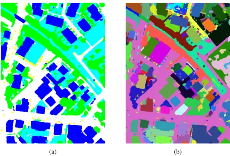
Figure 2: Each pixel in the generated image has been classified into six different classes (one class not present in the image).
Ground Truthis the desired output of the network, the correct answer that the network must achieve. In most cases the ground truth has to be created with considerable manual effort.
2.2
Concepts
Deep learningis a form of machine learning that consists of multiple layers of non-linear processes with modi-fiable parameters. Information is fed forward through the layers achieving multiple hierarchies of abstraction. Deep learning refers to large neural networks that employ supervised or unsupervised learning for their training.
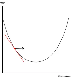
Supervised learning works by producing an error value as a result of a comparison between the output of the network and the desired output, or, ground truth. This error value is then back-propagated through the network in order to modify the networks parameters such that the error is minimized on the next pass. In a simplistic case, as seen in Figure 3, the error can be interpreted as a convex curve. Each point on the curve represents an error produced by the network as a function of its parameters. Using the negative gradient of the error with respect to the parameters allows a modification of the parameters in the direction of the minimum. This is commonly referred to asgradient descent and is a fundamental aspect of neural network training [3; 4].
Error
Parameters
Figure 3: The red line represents the gradient and the arrow represents the direction in which to modify the parameters in order to minimize error.
Unsupervised learningtechniques do not have any ground truth to derive an error. Error values are generated using a variety of different ways including probability distribution divergence [5] and pattern analysis [6].
CNNsor Convolutional Neural Networks are a type of neural network consisting mainly of convolution layers, hence its name. Aconvolution layer operates by traversing an image’s pixels using a kernel of a predetermined size. Thekernelis a block of weights, or parameters, that are multiplied to an image’s pixels and produce a value representing a pixel in a new image of some higher abstraction. Say we have an imageIand a kernelW of size3×3
then the operation to produce the new imageI∗would be as follows:
I∗ i,j= 3 X x=0 3 X y=0 Wx,yIi+x,j+y (1)
Often, as in many other neural networks a bias is added to the result.
Deconvolution layers also, and more correctly, known as transposed convolution layers, are present in image generation. Normally a convolution layer will reduce the spatial dimension and increase abstraction. Deconvolution layers tend to decrease abstraction into higher image dimension. This layer essentially performs the inverse of the convolution producing multiple pixel values given a single input pixel [7].
ReLUor rectified linear units are a method of introducing non-linearity into the feed-forward process of learning. It outputs the input value if it is greater than zero or zero, as can be seen in (2) [8]. This activation function is the one
most used in this work and generally follows a convolution layer.
f(x) =max(x,0) (2)
In a CNN, there is also commonly apooling layer, which reduces an area of pixels into an average (3) or into the maximum (4). Given a pooling size of2×2:
I∗ i,j= 1 4 2 X x=0 2 X y=0 Ii+x,j+y (3) I∗
i,j=max(Ii,j, Ii+1,j, Ii,j+1, Ii+1,j+1) (4)
Batch Normalizationis a process of normalizing the output of the preceding layer. It subtracts the batch mean and divides by the batch standard deviation. This allows for separation of learning between layers [9].
GANsor Generative-Adversarial-Networks consist of two networks competing against each other. One network, the discriminator, learns to identify real images from fake images. The other network, the generator, learns to generate images that look real. As the discriminator gets better at determining the false generated images the generator gets better at producing more realistic ones. Ideally the system converges when the discriminator can only tell with50%
certainty that a generated image is fake [5]. A common analogy is that of a counterfeiter making fake currency and a policeman identifying them. As the policeman learns to identify the counterfeit bills the counterfeiter learns to make them more realistic. Effectively, the generator learns to implicitly match the distribution of the real images. Upon convergence the generator can be used to produce realistic images within the distribution of the real images.
3
Related Works
Below we provide a brief overview of the state-of-the-art in the areas of (i) semantic segmentation, (ii) caustic removal, and (iii) urban and underwater scene and reconstruction.
3.1
Semantic Segmentation
Both in urban semantic segmentation and caustic labeling the goal is to achieve semantic labeling in order to proceed onto the next parts of the pipeline. The problem of semantic labeling has been explored through a variety of methods. Prior to deep learning, semantic labeling relied on hand engineered features. One of these methods proposed the generation of features that were classified into unary potentials then fed into conditional random fields (CRF), localizing the label and segmenting object instances [10].
Deep learning, over the past few years, has proved to be very effective at object recognition due to its ability to learn important features. Convolutional neural networks, first introduced by Yann Lecun in 1989, provide an effective method of extracting important features [11]. Girshick et al. use convulutional layers as a step within their system of segmentation [12]. One of the first cases of solely using deep learning in semantic segmentation was done by Long et al. in their work: ”Fully Convolutional Networks for Semantic Segmentation”. They employ a network that uses convolutional layers to abstract high level information which can then be used to infer a label map [13]. However, applying deep learning to semantic segmentation becomes a challenge as localized information is often lost in favor of high-level information. Chen et al. [14; 15] apply a CRF or a discriminatively trained domain transform to the model’s output to preserve edge information and to smooth semantic segmentation. Noh et al. [16] perform deconvolution to reach the original input resolution allowing the network to learn localization through deconvolution kernels.
Other works have the deep network perform the segmentation by preserving low-level information for the net-work’s segmentation process. SegNet [17], the network that inspired our work, consists of encoders and decoders that share pooling indices in order to preserve lower level information. Several other works apply this concept with slight variations [18; 19]. Pohlen et al. keep a single residual stream with information at the original resolution [20]. One network consists of holding previous pixel-specific layer activations within vectorized columns [21]. Another uses visual and geometric cues during unpooling [22]. Lin et al. use separate network paths to capture all available infor-mation from earlier layers [23]. A few high-performing networks base their work on the idea that a convolution has less contextual reach than assumed and they employ larger kernels [24], global image information [25], and different pooled feature maps [26; 27]. A major contribution to this approach in semantic segmentation was that of dilated
con-volutions. High resolution images are generally very heavy to process and depending on the kernel size there maybe be many operations that do not benefit to the abstraction of higher, larger context level features. Dilated convolutions introduced by Yu and Koltun allows the aggregation of multi-scaled contextual information without loosing resolution [28].
The previously mentioned works have a tendency to perform pixel-to-pixel level classification, this means that the classification can be done on a variable sized input to the model. Another approach is that of patch-to-pixel which occasionally performs well [29; 30; 31] but comes at the cost of processing time and neighboring contextual patch information.
Variants of the aforementioned network architectures have been employed in the context of semantic labeling of geospatial features each with unique advantages and trade-offs [32].
3.2
Caustic Removal
Although a plethora of work has already been reported on caustics generation, only a handful of techniques have been proposed for caustics removal; the majority within the context of image enhancement.
Trabes and Jordan [33] present a technique for tuning a sunlight-deflickering filter for moving scenes underwater. They propose a continuous parameter optimization inside a basic filter, which employs feedback in order to improve the performance. As reported in their paper there is a high sensitivity of the filter’s performance to badly optimized parameters and in particular, the segmentation parameter which is part of the objective function in the optimization.
A different approach was presented by Gracias et al. [34]. The authors present a mathematical solution which involves calculating the temporal median between images within a sequence. A strong assumption of this work, is the fact that feature matching ( a Harris corner detection variant established by Gracias and Santos-Victor [35]) is employed for the formation of the sequence which makes this approach very susceptible to the light variations in the images and in particular caustics effects. This work has since been extended in Shihavuddin et al. [36] by proposing an online sunflicker removal method which treats caustics as a dynamic texture. As reported in the paper this only works if the seabed or bottom surface is flat. Similar approaches have also been proposed for general cases of dehazing and descattering of images [37; 38; 39].
Schechner and Karpel [40] propose a method based on processing a number of consecutive frames. These frames are analyzed by a non-linear algorithm which preserves consistent image components while filtering out fluctuations. Their proposed method however does not take into account the camera motion which almost always leads to
registra-tion inaccuracies.
In order to avoid registration inaccuracies Swirski and Schenchner [41] present a method for removing caustics using a stereo-rig. The stereo cameras provide depth maps which can then be registered together using ICP (Iterative Closest Point; a technique for aligning multiple geometries to one another). This again makes a strong assumption on the rigidity of the scene which is seldom the case in underwater.
Trabes and Jordan, propose an approach which employs optical flow techniques and curvature predictions of pixel traces during the motion [42]. As with the aforementioned technique there are strong assumptions on the small motion and color constancy between consecutive frames.
3.3
Reconstruction
Reconstructing caustic scenes has been rarely attempted. Some tried using structure from motion techniques with poor results [43; 44]. Although the scene is static and the camera is moving smoothly the variation in illumination throws off the feature matching algorithm.
Urban reconstruction, on the other hand, has been an active research area since the early 80s hence it is no surprise that a vast body of work exists. A comprehensive survey of state-of-the-art can be found in Musialski et al. [45] where techniques proposed over the past few years are categorized according to the objective, type, and scale of data.
There are techniques which use symmetries and regularities in the geometry. Zhou et al. [46] proposed an auto-mated system which given theexact bounding volume of a buildingcan simplify the geometry based on dual contouring while retaining important features. Using this technique the authors were able to simplify the original geometry con-siderably. On a similar line of research, Verdie et al. [47] proposed a method which produces excellent reconstructed models from pointcloud data which can also produce models at different levels-of-detail. Although tghbese techniques produce impressive results, they do require considerable user interaction during the pre-processing stage typically in the form of carefully identifying the objects’ points.
Other techniques aim for full-automation and are therefore entirely data-driven. One such example is the work of Poullis et al. [48] where pointcloud data is converted automatically to polygonal 3D models. This technique is applicable directly on the raw pointcloud data without requiring any user interaction. Later, Poullis [49] extended the work to include a fast boundary refinement algorithm based on graph-cuts which was used to refine the boundaries. Overall, these techniques scale well with vast amounts of data however this comes at the cost of increasing the difficulty of enforcing symmetry constraints such as the Manhattan world assumption. In other words, larger areas can be
processed but the generated models are noisier than the previous approach of using regularities. A solution to this side-effect was proposed by Arikan et al. [50] where a system for generating polyhedral models from semi-dense unstructured point-clouds was developed. Planar surfaces were first extracted automatically based on prior semantic information, and later refined manually by an operator.
Finally, a rather different approach was proposed by Xiao et al. [51] where the authors used inverse constructive solid geometry to address the reconstruction problem. Rather than using boolean operations on simple primitives to generate a complex structure, they start off with a point cloud representing the indoor area of a structure and decompose that into layers which are then grouped into higher-order elements. This works very well for highly regularized scenes such as indoor spaces however it does not produce useful results for large-scale outdoor areas.
orthophoto of the historical city Vaihingen, Germany, has an average resolution2000×2500, and a sampling density of 9cms. For each IRRG-depth image pair, a ground-truth image is also provided showing the manually assigned per-pixel classification into six classes: (a) buildings (blue), (b) roads (white), (c) trees (green), (d) red (clutter), (e) low vegetation/natural ground (cyan), (f) cars (yellow). The ‘clutter’ class contains areas for which a class could not be assigned e.g. water, vertical walls, areas where computing the depth (SfM+MVS) has failed, etc. The ‘low vege-tation/natural ground’ class contains areas on the ground covered by vegetation other than trees such as low bushes, grass, etc.
4.2.2 Network Architecture
A number of network architectures have already been reported for semantic labeling. State-of-the-art performance is generally associated with how deep and wide the networks are. However this introduces a significant drawback since the deeper/wider the network, the larger the number of parameters that need to be optimized during the training phase; and although training time is often overlooked it is an important factor when assessing the overall applicability and deployment of a network architecture.
Furthermore, when dealing with deep network architectures the resolution of the input data deteriorates as the data progresses through to the deeper layers. This often materializes as non-smooth and noisy predictions during the final upsampling stages in the network. A common way of addressing this is to smooth the predictions using a conditional random field based post-processing approach.
In our work, we propose a distinct network architecture which uniquely combines the strength of convolutional au-toencoders with feed-forward links in generating smooth predictions and reducing the number of learning parameters, with the effectiveness which cardinality-enabled residual-based building blocks have shown in improving prediction accuracy and outperforming deeper/wider network architectures with less learning parameters, to address the afore-mentioned limitations of existing state-of-the-art. The closest related work in terms of network architecture is with SegNet presented in [17] where the concept of feeding forward pooling indicesfrom the encoders to the decoders was introduced, and the ResNeXT building blocks presented in [53] where the concept ofcardinalitywas introduced and was shown that increasing cardinality was more effective than deeper/wider network architectures. Hence, to summarize, the topology of the proposed network resembles that of SegNet with the main differences that the feed forward connections are between feature maps (as opposed to pooling indices) and each encoder or decoder consists of a ResNeXT block.
Data Input
Our network takes in patches of150×150 that are selected from the 16 available training images. We select random points within each image and construct a patch around each point. This decision is based on the observations that (a) given the high resolution of the images random sampling results in patches with large content variability, and (b) due to this large content variability (i.e.16×5million patches per2K×2.5Kimage) the overall accuracy on the training images can be used as a proxy (i.e. almost the same) for the overall accuracy on the validation/testing images. Each patch is represented as a3-dimensional tensor containing the IRRG data and the corresponding depth map. We select 2 patches from each of the 16 image-pairs for each batch resulting in a total batch size of32different patches of150×150×4. Class balancing (near equal training samples from different classes) was also tested but did not show any improvement in learning which could be attributed to the large amount of data used.
4.2.4 Validation
The proposed network was validated against the additional 17 image pairs available for testing for which ISPRS did not make the ground truth publicly available. In order to generate our test images we employ a sliding window approach that evaluates each patch at intervals of10pixels in the diagonal in order to minimize context based errors. Our results are then averaged into one final image.
The network’s performance is measured in terms of Precision (P), Recall (R), andF1score which are defined as,
P = tp tp+f p R= tp tp+f n F1= 2× P×R P+R (5)
wheretpindicates the true positives,f pindicates the false positives, andf nindicates the false negatives.
Table 1 shows the evaluation of the overall classification results for the 17 test images and as it can be seen the overall accuracy is89.2%. At the moment of writing the highest overall performance is91.2%from a deep fully-convolutional neural network (FCN) ensemble followed by post-processing using a fully connected CRF (F-CRF) for further improving the results. Close inspection of our evaluation results indicate that there is about a1−2%variation between our classification (buildings, trees, roads, and clutter) and the state-of-the-art, and a highest difference of about
4%for the car class. We can only assume that the ensemble consists of networks tuned at different scales although no publication is available to corroborate this. Despite the lower overall accuracy on the entire test dataset, there are cases where the overall accuracy of our network outperforms the state-of-the-art, such as test images V-0004 shown in Figure 14b. This can be attributed to the fact that our network is under-performing (compared to state-of-the-art) in
classifying cars so in the presence of many cars in the test image the overall accuracy drops; similarly, in cases where not many cars are present in the test images the overall accuracy increases and surpasses other competing networks. Figures 6 and 7 show the results for two of the 17 test images, namely V-0003 and V-0012.
Furthermore, we have also tested variations of the proposed network architecture. In particular, we have ex-perimented with (a) data augmentation, (b) atrous convolution [54], (c) CRF-based post-processing. There were no improvements in the overall accuracy which was in fact lower in the range of84−89%. For the CRF-based post-processing the results were almost identical i.e. 89.1%which verifies the claim that deep autoencoders with feed-forward links between feature maps produce smooth, non-noisy results.
ref.→
pred.↓ roads building low veg tree car clutter
roads 0.937 0.023 0.031 0.007 0.002 0.000 building 0.048 0.931 0.018 0.003 0.000 0.000 low veg. 0.047 0.015 0.800 0.138 0.000 0.000 tree 0.010 0.003 0.077 0.911 0.000 0.000 car 0.209 0.056 0.006 0.003 0.726 0.000 clutter 0.379 0.345 0.016 0.003 0.054 0.204 Precision 0.896 0.949 0.847 0.865 0.862 0.979 Recall 0.937 0.931 0.800 0.911 0.726 0.204 F1 0.916 0.940 0.823 0.887 0.788 0.338
Table 1: The overall evaluation of the classification results for the 17 test images for which ground truth was not provided. The network performance statistics were computed by and provided by the ISPRS Working Group II/4 organizers as part of their urban classification benchmark. All shown values are percentages.
(a) (b) (c)
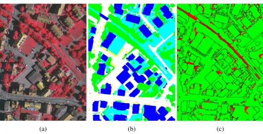
Figure 6: The evaluation result for one of the 17 test images. Resolution1887×2557(a) Satellite image of the urban area V-0003. (b) Generated label map. (c) Red/green image, indicating wrongly classified pixels. The railroad is classified incorrectly as a low vegetation instead of clutter.
(a) (b) (c)
Figure 7: The evaluation result for another of the 17 test images. (a) Satellite image of the urban area V-0012. (b) Generated label map. (c) Red/green image, indicating wrongly classified pixels.
4.2.5 Network Comparison
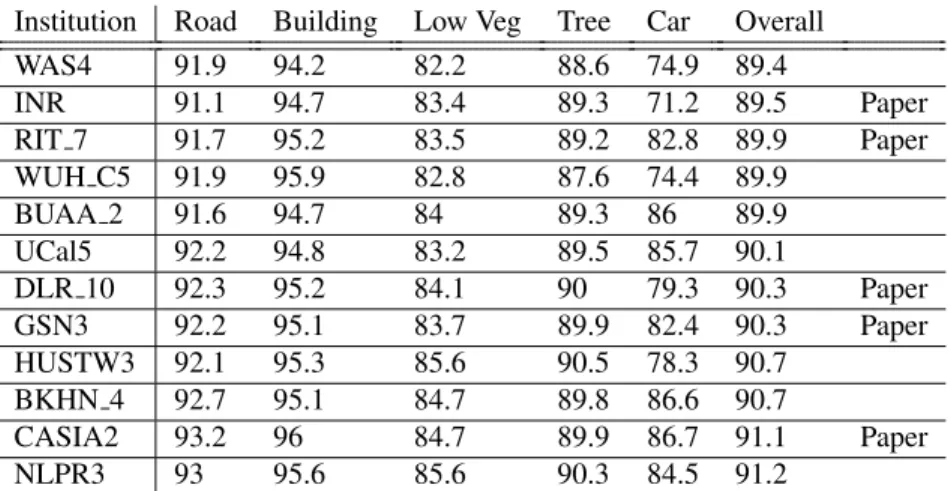
Results on this dataset are posted to the public on the ISPRS benchmark website. From there we could gather information about higher performing networks, if the authors have made that information available with their submis-sion. Unfortunately not many of the highest performing networks give detailed information, although a brief abstract of their work is sometimes found. As mentioned earlier, at the time of submission, the highest performing network achieved accuracy of91.2%. This network, labelled NLPR3, is defined as an ensemble of fully-convolutional neural networks followed by fully connected conditional random fields. The use of ensemble networks generally means that the size of the whole system is significantly larger thus also means more training time and memory.
We evaluate other networks that made their work available and that performed better on the dataset compared to our network. We do this in an attempt to further understand how improvements can be made or to justify and explain why other networks had higher accuracy.
Liu et al. present the second best performing network in table 2. Their network comprises of a similar encoder-decoder structure. However they implement a cascade of multi-scale contexts appended to their encoder. They do this in order to distinguish confusing man-made objects present in the scene. Their work is well explained a performs extremely well given they do not use and depth data. Their model is appended onto existing encoder and so its size is not much greater than any of the current state of the art networks. Unfortunately their work was published later than our submission and could not be used as insight to any valuable decision [55].
Wang et al. also perform exceptional results with their GSN submission considering they forgo the use of DSM in their training. Their model consists of using a gated convolutional network that allows more effective information to
be passed from feature maps of different sizes. The only downside of their work is the size of their network as it bases off of ResNet and hence requires a lot of memory and training time [56]. Marmanis et. al achieve similar performance to GSN with their DLR 10 submission. They make use of DSM and nDSM and implement an explicit edge detection in the intial phases of their network. They also make use of an ensemble network meaning their system is very large and requires a lot of memory to run in parrallel or time to run sequentially [57].
The RIT submission explores networks that consist of fusing branches of the convolutional streams and then concatenating those features for further processing to obtain the final output result. Some of their networks perform well and require little training parameters however their most performing one, the composite fusion network, requires larger branches of network streams meaning more parameters and longer computation time. They also make use of DSM and nDSM in their network [58].
Finally the INR submission makes use of DSM in a similar network to SegNet but instead of upsampling and convolving they unpsample every encoder result and then contantenate everything into a final output. This results in a network with fewer parameters [59].
It is important to note that the ground truth data was done by hand and as such it is prone to human error which is commonly said as1%−5%. This simply means that many different networks could perform better or worse given a different dataset, and given different annotations for the ground truth.
Institution Road Building Low Veg Tree Car Overall
WAS4 91.9 94.2 82.2 88.6 74.9 89.4 INR 91.1 94.7 83.4 89.3 71.2 89.5 Paper RIT 7 91.7 95.2 83.5 89.2 82.8 89.9 Paper WUH C5 91.9 95.9 82.8 87.6 74.4 89.9 BUAA 2 91.6 94.7 84 89.3 86 89.9 UCal5 92.2 94.8 83.2 89.5 85.7 90.1 DLR 10 92.3 95.2 84.1 90 79.3 90.3 Paper GSN3 92.2 95.1 83.7 89.9 82.4 90.3 Paper HUSTW3 92.1 95.3 85.6 90.5 78.3 90.7 BKHN 4 92.7 95.1 84.7 89.8 86.6 90.7 CASIA2 93.2 96 84.7 89.9 86.7 91.1 Paper NLPR3 93 95.6 85.6 90.3 84.5 91.2
Table 2: Results of highest performing systems submitted by each institution that performed better that our network. The last column dictates whether the institution attached a paper to their submission.
4.3
Network Design
4.3.1 Structure
Our initial attempts at urban classification consisted of building a network that would identify a single pixel on each forward pass. The reasoning was that as a patch is convolved the data is abstracted from surrounding pixels accumulating into a very condensed array of information that would give an accurate classification of that single pixel. While this proved somewhat true final results were not very good in boundary delineation. We assume this is because a boundary can delineate two classes within one pixel difference, hence two very similar condensed arrays could represent two different classes.
We then attempted a cascade method which consisted of models that were unique to each class. Since each model would produce a probability of a pixel being a specific class or not we could then find the class with the highest probability. Our system consisted of first running the network on input patches of size55through a vegetation class network. We would then produce the output from that network and concatenate it to the input and pass it through the tree class network. We proceeded the same way for cars, buildings, and finally ground. While this improved boundary delineation and each model converged faster it still took hours for testing of a single image. We also determined that cascading also ended up accumulating errors.
Our next attempts consisted of simple convolutions followed by deconvolutions. This produced faster results but boundary delineation was not good. Further research pushed the idea to have links between each encoder and decoder block. Around this time ResNeXt [53] was a popular well performing network. Applying it to our network improved performance without increasing parameter size and convergence time. This architecture proved effective and yielded good results so we settled on that.
4.3.2 Parameters
Having such a large network with so many parameters proved extremely difficult. Parameters defining convolution kernel sizes were chosen based on similar models created by other researchers. Slight changes were made but no significant improvements were noted and so some parameters were set for symmetry and ease of presentation. Patch size was determined by testing different models going from55×55to256×256, at different intervals. As patch size increased our batch size had to decrease (due to our hardware memory limitation) during training and testing. Once we reached a patch size of150we noted that convergence times were significantly greater and did not justify the slight increase in performance. We also noted that as batch size decreased classes with smaller pixel coverage (such as
cars) performed worse. We later assumed that as batch size decreases variation in pixels does too, meaning that each backward pass generalizes less to less consistent pixels. Class balancing may have been a suitable course of action at this stage if we had thought of it.
Parameters were iterated through randomly, and occasionally manually tested based on educated assumptions. Through an empirical study of the tested parameters we reached a model that performed well and we were able to move onto reconstruction of the urban scenes.
4.4
Urban Reconstruction
The result of SegNeXt is a per-pixel classification into one of the six classes i.e. cars, buildings, trees, roads, low vegetation, and clutter. Next, the 2D per-pixel classification image is used as a proxy to cluster the 3D points in the depth map. This results in a cluster map shown in Figure 8b containing disjoint, contiguous regions. Based on the cluster’s classification, an automatic per-class reconstruction is performed to generate the 3D models for each class. Finally, the 3D models are fused together to create a complete virtual representation of the entire site.
(a) (b)
Figure 8: (a) SegNeXt predictions for test image V-0003. (b) Agglomerate clustering of neighbouring points in (a) of the same class.
4.4.1 Buildings
Perhaps one of the most important aspects in urban reconstruction is the accurate modeling of buildings where large depth discontinuities appear as jagged edges in the captured remote sensing data. Typically, a refinement and smoothing operation is performed as a first step prior to further processing.
5
Case Study #2: Caustics Removal and Underwater Scene Reconstruction
5.1
Overview
In order to improve reconstruction quality and accuracy of underwater scenes the first step is to identify caustics and remove them. Caustic detection and removal from real images was attempted using a Convolutional Neural Network with an architecture similar to that of a Convolutional Autoencoder reported in [60], where the first layers perform convolution, and subsequent layers perform de-convolution. CNNs are a natural choice when dealing with images; however, unlike traditional convolutional networks, which rarely attempt pixel level classification, we require an architecture that produces images of sizes matching input image sizes, hence the need for de-convolution layers. In order to perform the removal of caustics on a video we required the network to perform on each frame as fast as possible and hence be very small. SfM can then be used on the resulting images to produce a higher quality and more accurate reconstruction.
Images with caustic are fed into a first network called SalienceNet which outputs a salience map corresponding to the probability of a pixel being a caustic. This salience map is then concatenated to the original image and fed into another network, DeepCaustics, where the caustics are removed from image producing a caustic free image that can be used for more accurate reconstruction. This section of work has been published in the IEEE Journal of Oceanic Engineering [61].
5.2
SalienceNet
5.2.1 Dataset
Since there is no ground truth data available for real world underwater caustics, we decided on supervised learning using synthetic data for ground truth. Using sample underwater video images with caustics we created a set of synthetic data using 3D objects for underwater seabeds, multiple lighting and global illumination for rendering caustic effects with the virtual camera located below the water surface as in real world shallow water imaging. In addition to the rendered caustics images, we rendered the masks containing confidence values of a caustic occurring at a pixel and also corresponding caustic-free images. The dataset was created with Arnold Renderer using photon mapping [62] in Autodesk Maya 2017. The masks containing the confidence values are used as ground truth to the SalienceNet. The input to SalienceNet is a rendered RGB image containing caustics of an underwater scene. The network operates on a batch of32images of size400×400. Each pixel of the output image takes a value in the range of[0,1], corresponding
to the confidence of caustics occurring at that pixel, hence the output is a single channel black and white image.
5.2.2 Network Architecture
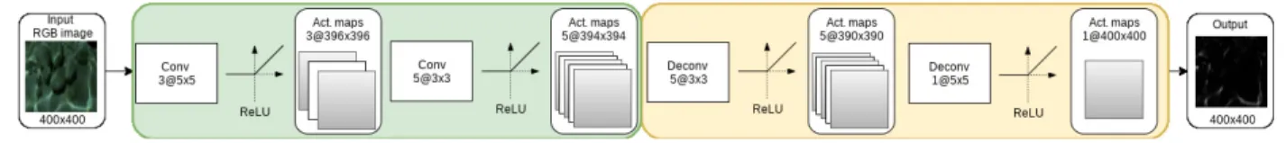
After extensive experimentation, we have concluded that the network architecture with the optimal performance relative to size consists of four hidden layers; the first two consisting of 3 and 5 convolution filters respectively, and the last two consisting of 5 and 1 de-convolution filters respectively. The filter sizes are5×5,3×3,3×3,5×5in each layer respectively. This results in a total of2×(5×3×3) + (4×5×5)weight parameters and8 + 6bias parameters, for a total of204 parameters to be learned. Such a small number of parameters means that each forward pass on the network during testing will be extremely fast. This means that a whole video sequence can be processed almost in real-time. Each convolution/deconvolution in the network is followed with a ReLU activation unit [63]. Initially, sigmoid activation units were used in the last layer to ensure that the final output is in the range[0,1]however, our experiments have shown that ReLU units perform better [they still map the output in the range [0,1]provided the input data falls within the manifold learned] and, in addition computing the gradients becomes more stable during back-propagation i.e. no ‘squashing’ leading to vanishing gradients. Adding more units and/or more layers has also been tested, but with no improvements important enough to justify longer processing times. Larger filter sizes were also tested, but yielded blurry results. In order to get reasonable results with an initial layer consisting of larger filters, more layers with decreasing filter size were needed, but this required a reduction in the size of the images in the data set due to memory constraints, and added no significant advantages. A diagram of the network’s architecture, chosen based on all the experimental evaluations and considerations described above, is shown in Figure 16
Figure 16: SalienceNet: a 4-layer CNN consisting of 2 convolutional layers followed by 2 deconvolutional layers.
Thus, the network models the following operation,
ReLU(Ψ−1
∗ReLU(Ψ−1
∗ReLU(Ψ? ReLU(Ψ? X))))→Φp (6)
where p is a pixel andΦis its saliency value. In the above equation X denotes the input data,Ψdenotes a convolu-tion kernel,?denotes the convolution operation,Ψ−1
denotes a de-convolution kernel,∗denotes the de-convolution operation, andReLU(.)is the rectified linear unit activation function.
the saliency value the higher the confidence of caustics occurring at that pixel.
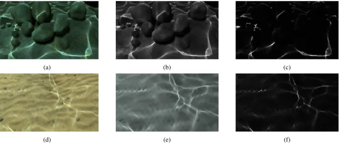
Figure 17: Color transfer [64] and histogram matching [65] of the luminance channel are applied to the real images in order to make the real images fall within the manifold learned from the training images and remove possible bias to colors. The images showing the luminance are shown as grayscale images.
5.2.3 Training
The network was implemented and trained using Theano API [66] on a set of 500 synthetic images. 60 synthetic images were reserved for validation. Figure 18 shows example pairs of input and ground truth images used for training the SalienceNet. The left column shows the rendered RGB image used as input and the center column shows the rendered caustics masks using global illumination and final gathering. Indirect lighting results in almost all pixels having a non-zero brightness value. The right column shows the thresholded caustics mask used during training as the ground truth saliency map.
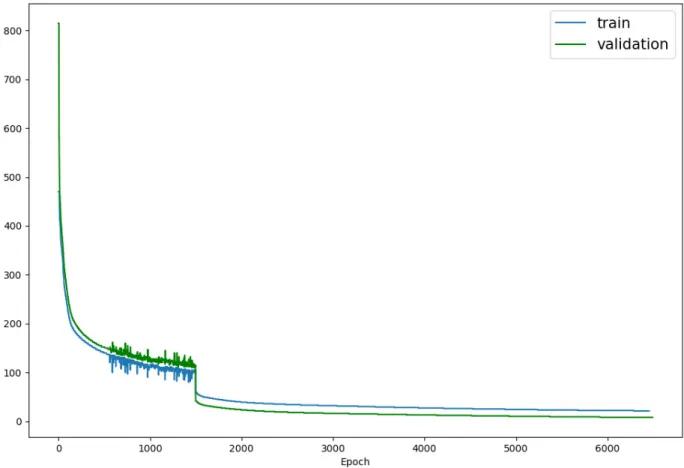
Although a synthetic data set was used for training, we were ultimately interested in the network’s performance on the real data set which can be considered a form of transfer learning. The network was trained for1500epochs at a learning rate of0.001, which required approximately9.5hours of training on an GeForce GTX 1070 8GBVRAM GPU, followed by an additional5000epochs at a learning rate of0.0001. A batch size of32was used. We also experimented with dropout [67], but no improvements were noticed, which indicates that overfitting was not a problem during the training process. Figure 19 shows the cost function error, modeled as a Mean-Squared Error (MSE) for 6500 epochs. Mean-Squared Error is the sum of squares of difference in pixel values from the ground truth and our predicted results.
(a) (b) (c)
(d) (e) (f)
Figure 18: Examples of the training data. Left column: The rendered RGB image used as input to SalienceNet and DeepCaustics. Center column: The rendered caustics masks using global illumination and final gathering. Indirect lighting results in almost all pixels having a non-zero brightness value. Right column: The thresholded caustics mask used during training as the ground truth saliency map.
The formula is as follows,
1 n n X j=1 (ptruthij −p pred ij ) 2 (7)
wherepijis a pixel in theithrow andjthcolumn in the ground truth image or the SalienceNet image result.
5.2.4 Validation
As previously mentioned our main goal is to transfer the learning to real data sets. Towards this goal of transfer learning, due to the color variance of the water, seabed and caustics, the real images are first preprocessed such that the color space manifold matches that of the training set. Given a real image the preprocessing involves performing color transfer described by Reinhard et al. [64], converting from RGB color space to Luv, performing histogram matching as done by Coltuc et al. [65] on the luminance channel L, and converting back to RGB color space. Figure 17 shows an example of this process.
Following the training of SalienceNet using synthetic data, we processed a number of varied real world underwater videos through this network and obtained very good results. Although we cannot directly assess the accuracy of the SalienceNet in removing caustics given the lack of ground truth on the real images, we do evaluate its performance in terms of the reconstruction metrics described in Section 5.5. In other words, the metrics used to evaluate the reconstruction serve as a proxy for determining the performance of the networks. Five images from distinctive videos taken underwater are shown in the left column Figure 20 and the resulting saliency maps produced by SalienceNet are
Figure 19: SalienceNet Cost Function Error (training and validation curves are almost identical): First1500epochs at a learning rate of 0
.001and the next 5000 epochs at a learning rate of0.0001. The cost function used is Mean-Squared Error (MSE).
shown in the right column.
5.3
DeepCaustics
5.3.1 Dataset
The input to DeepCaustics is the pair of an image containing caustics and the saliency map generated by SalienceNet. The two are first coupled together into a 4-channel RGBA format where the fourth channel contains the saliency value for the corresponding pixel. The ground truth used for training is a rendered caustic-free image corresponding to the synthetic input images. An example is shown in Figure 21. The network operates on a batch of16images of size
Figure 20: (right) The saliency maps generated by SalienceNet for the five real images (left) from distinctive videos taken underwater containing caustics of varying frequencies and shape.
(a) (b) (c)
Figure 21: Examples of the training data for DeepCaustics. (a) The rendered RGB image used as input to DeepCaustics. (b) The saliency map generated by SalienceNet. These two images [(a), (b)] become the input to the DeepCaustics network. (c) The ground truth used for training is a rendered caustic-free image corresponding to (a),(b).
5.3.2 Network Architecture
After extensive experimentation, we have concluded that the network architecture with the optimal performance consists of six hidden layers; the first three consisting of 4, 2, and, 7 convolution filters respectively, the last three consisting of 7, 2, and 3 de-convolution filters respectively. The filter sizes are3×3,7×7,3×3,3×3,7×7,3×3in each layer respectively. This results in a total of(4×3×3)+2×(2×7×7)+2×(7×3×3)+(3×3×3)weight parameters and(4 + 2×2 + 2×7 + 3)bias parameters, for a total of410parameters to be learned. Similarly to SalienceNet, after each [de-] convolution in the network follows a ReLU activation unit [63]. Figure 22 shows the architecture of the DeepCaustics network. An important observation first reported by [68] which was also confirmed during our experimentation is that scaling up the number of activation maps while scaling down the kernel size produces considerably better results.
Figure 22: DeepCaustics: a 6-layer CNN consisting of 3 convolutional layers followed by 3 deconvolutional layers. A ReLU activation unit follows each [de-]convolution operation.
5.3.3 Training
The colour transfered pre-processed images along with the saliency values generated by SalienceNet form the input for the trained DeepCaustics. Again, the expected output is a caustic-free image. The network is trained using 180 synthetic image-pairs, and 20 synthetic image-pairs for validation. We trained the DeepCaustics network on the same hardware as for SalienceNet. Figure 23 shows the cost function error, modeled as a structural similarity index (SSIM); a quality measure of one of the images being compared, provided the other image is the ground truth.
SSIM evaluates images accounting for the fact that the human visual system is sensitive to changes in local structure. SSIM is implemented by creating patches from the ground truth images (y) and the predicted images generated from DeepCaustics (x). For each patch we calculate the SSIM:
SSIM(x, y) = (2µxµy+C1) + (2σxy+C2) (µ2
x+µ2y+C1)(σx2+σy2+C2)
(8)
such thatµis the average value of the patches,σ2
is the variance,σxyis the covariance between patchesxandyand
σis the standard deviation of the patches.
Our experiments have shown that it performs better than MSE in terms of network training as it has been also discussed by Zhao et al. [69]. The network was trained for2700epochs with a learning rate of0.001. The choice of
2700epochs is somewhat arbitrary; the learning curve shows that much of the training progress occurs within the first
80epochs.
Figure 23: DeepCaustics cost function error. The cost function used is Structural Similarity index (SSIM). SSIM is a quality measure of one of the images being compared, provided the other image is the ground truth. SSIM evaluates images accounting for the fact that the human visual system is sensitive to changes in local structure.
5.3.4 Validation
As previously mentioned this work is motivated by the real world challenges in underwater archaeology. Pro-cessing videos for underwater entities in the presence of caustics is very hard. Figure 24 demonstrates that using the proposed approach successfully removes the caustics from the images therefore allowing more accurate further processing towards 3D reconstruction. In the first column we show five sample frames from real world RGB videos containing caustics of varying characteristics. When these images are input to DeepCaustics along with their saliency maps generated by SalienceNet the results obtained are shown in Figure 20. The second column in 24 shows the five RGB images after color transfer and histogram matching. In the third column we show the results generated by
DeepCaustics on the original images i.e.withoutany color transfer and histogram matching operations. As expected the network does not perform well for any images which fall outside the learned manifold. The last column shows the caustic-free images generated by DeepCaustics on the color matched RGB images shown in the second column. The caustics have been successfully removed and therefore further processing with structure-from-motion and multi-view stereo techniques becomes possible.
Figure 24: First column: The original RGB images for five selected scenes which contain caustics of varying characteristics. Second column: The RGB images after color transfer and histogram matching. Third column: The results generated by DeepCaustics on the original images withoutcolor transfer and histogram matching i.e. first column. Fourth column: The caustic-free images generated by DeepCaustics on the color matched RGB images shown in the second column. The caustics have been successfully removed and therefore further processing with structure-from-motion and multi-view stereo techniques is possible.
As said earlier, the images shown in the figures are individual sample frames taken from videos. We actually carry out the process for all frames in the video. Although there is no temporal information being taken into account when processing the video i.e. each frame is individually processed, we have seen that the resulting caustic-free video is smoothly varying and consistent across sequential frames. Figure 25 shows the saliency maps and caustic-free images are consistent between frames 25, 30 although there is considerable camera motion as well as caustic motion between
them.
(a) (b) (c)
(d) (e) (f)
Figure 25: Frames 25 and 30 are processed independently i.e. no temporal information is used. The saliency maps and caustic-free images are consistent although considerable motion [camera, caustics] has occurred between the two frames.
An extreme case of caustics produced by turbulent water motion which causes caustics of varying frequencies which are not well defined in terms of structure is shown in Figure 26. Similarly Figure 27 shows another complex example of caustics appearing on rocks with barnacles. Despite the complexity of the scene the proposed approach is able to correctly classify pixels as caustics/non-caustics and remove them. An example of this is the shadow of the boat being consistently classified as non-caustic throughout the video sequence.
5.3.5 Network Comparison
An in depth evaluation of the technique on other datasets was performed at the Cyprus University of Technology. The evaluation explains how this technique improves the images and provides more robust feature matches between image pairs [70]. Unfortunately it is very hard to compare this method with other techniques as there is no public reference dataset that can be used as a benchmark to our knowledge, and, other techniques are hard to replicate or get a hold of. However we attempt a comparison of different systems by exploring their published work.
In Trabes et al.’s work they establish a sunlight-deflickering filter for scenes that are very similar to those in our work. While they explain how there method works they do not provide very much visual evidence of an effective algorithm. Because of their feedback system their algorithm is stable to fluctuating changes in scene illumination and structure. There method does not require as much resources as other systems yet to perform well it must run consistently to determine its new parameter values. Another limitation to their work is that they require future frames for a section of their algorithm meaning it cannot work on an on-line setting [33].
Another method uses multiple frames a adjusts them through the use of temporal information. However, in order to make use of the temporal information they must be aligned and to do so requires a robust feature matching algorithm. Given the intensity of the caustics then the feature matching algorithm could fail and the method would not work [34]. Several techniques that involve temporal information generally have significant disadvantages relative to our work. Schechner’s technique unfortunately does not consider changes in camera movement and as such provides images that would not help much for later reconstruction [40].
Shihavuddin’s approach relies on previous frames but not future frames. Their mathematical approach is not affected by camera motion and works by predicting the caustics in the coming frame. While their method is effective it requires around6seconds per frame, thus proving to be slow [36].
3Deflicker from motion by Swirski method is perhaps the most performing however it requires stereo cameras which prevent it from working on existing monocular video. It also requires expensive and specific technology [41].
(a) (b) (c) (d)
Figure 26: An extreme example of caustics caused by turbulent water movement. (a) The RGB image. (b) The color transferred images. (c) The saliency map generated by SalienceNet. (d) The caustic-free image generated by DeepCaustics.
(a) (b) (c) (d)
Figure 27: Another complex example of caustics appearing on rocks barnacles. (a) The original RGB image. (b) SalienceNet’s result. (c) Color-inverted saliency map. Note that objects like the shadow of the boat are consistently classified as non-caustics throughout the video sequence. (d) The caustic-free image generated by DeepCaustics. Note the occasional loss of color information due to processing.
5.4
Network Design
5.4.1 Structure
When exploring different structures for our system we had to stay within our most important constraint: size. The smaller the network the faster our forward pass and the more effective our system can be in real-time. This led to a network that would not surpass the 10 layers and where operations consisted of significantly small kernels. A smaller
network also reduces overfitting which is crucial when dealing with transfer learning as in this case.
One critical design choice with regards to our structure was having two different networks instead of a single one. Our main argument is, again, that of working with transferred learning. By sequentially breaking the process we ensure that the learning is transferred correctly onto real-world data in a more controlled manner minimizing a potentially unseen cascading error.
5.4.2 Parameters
In order to find the right parameters for our networks we went through several trials. We ran our networks for 200 epochs and selected the best parameters based on error, prediction results, and number of parameters. Our errors can be seen in Table 3 with bold values representing our selections of each network.
Activation Kernel SalienceNet (MSE) DeepCaustics (SSIM)
3,3 3,3 86.56 0.1628 3,5 5,3 94.50 0.1265 3,5,10 15,7,3 103.85 0.1947 4,2,7 3,7,3 115.56 0.0361 5,10,20 5,9,5 91.06 0.0359 5,10,20 15,9,5 116.55 0.0251 5,12,24 27,13,5 97.32 0.0245 20,10,15 3,7,5 71.06 0.0120 20,10,15 5,13,7 76.66 0.0179
Table 3: Errors for different network parameters after 200 epochs. Note that SalienceNet and DeepCaustics have different error functions, hence the different ranges of values. Activation column represents the feature maps for each layer with respect to the Kernel values squared for the kernel size. The first row would be a network of two layers, with the first layer consisting of 3 activation maps and a kernel size of 3x3. The second layer would also have 3 activation maps and a kernel size of 3x3.
When selecting our SalienceNet we noticed improvement when increasing layers and layer complexity however the trade off between the error and the number of parameters was too large to ignore. We also noticed that our last two tests, while having low error, over fit towards the artificial data producing erroneous salience images for real images. A similar issue happened with our DeepCaustics network. Our tests removed inefficient parameters but also permitted us to observe how differences in kernel size and how depth affected our results. Again increased complexity provided lower error but this meant more parameters and often over fitting.
The proposed approach has been extensively tested on real videos of underwater scenes containing caustics. The videos contain a large variability in terms of the color, the frequency of the caustics i.e. wave speed and formations, the background i.e. geometry and color [sand, rock, barnacles, etc], and shape i.e. wave interference.
5.5
Reconstruction
In order to evaluate the results of our method we constructed a 3D object from a sequence of thresholded images and a sequence of images generated by DeepCaustics. This was done to demonstrate the effectiveness of our method relative to a simple thresholding of brightness in an image.
(a) (b) (c)
Figure 28: Examples of the images that are used in the 3D reconstruction. (a) The original RGB image. (b) The thresholded image. (c) DeepCaustic generated image placed back into its original colorspace.
The 3D object consists of a block of concrete found underwater. We construct a 3D object using Agisoft’s Photo-Scan (SfM) from our image sequences, then we extract planes from four different sides of the cube. From these planes we calculate (1) a surface fitting metric evaluating the “smoothness of our reconstruction” and (2) the orthogonality with all adjacent faces. All faces, except opposing ones, should have an orthogonality of 90 degrees to represent how they are perpendicular. Opposing faces should be parallel. The metrics are defined below.
Surface fitting metric
A surfaceΠis reconstructed and a planeΠf itted =hα, β, γ, δiwith normalNΠf itted =hnx, ny, nziis fitted on
the resultingℵ3D points. The plane fitting is performed using RANSAC and the average errorEavgand average
RM SEis computed as follows, Eavg= ℵ X i=0 |δ−(α× ℵx i +β× ℵ y i +γ× ℵ z i)|/||ℵ|| (9) RM SE= s Pℵ i=0{δ−(α× ℵ x i +β× ℵ y i +γ× ℵzi)}2 ||ℵ|| (10)
We reconstruct several different planar surfaces shown in Table 4 and perform plane fitting using RANSAC. This metric is measured as the distance of all points from the fitted surface in terms of the average errorEavg and the
Threshold DeepCaustics
Top 0.8276 0.9690
Front 0.9965 0.9974
Left 0.9787 0.9882
Right 0.9207 0.9564
Table 4: Surface fitting metric for different faces of the 3D reconstructed cube.
Top Front Left Right
Top - 90.99 91.86 85.76
Front 56.65 - 92.29 56.28
Left 56.98 57.27 - 31.75
Right 57.26 52.83 35.47
-Table 5: Orthogonality between different faces of the 3D reconstructed cube. The upper triangle of the table are re-sults from images processed with DeepCaustics. The lower triangle contains results from images where brightness has been thresholded.
Orthogonality metric
A set of perpendicular surfaces are reconstructed and four planes Π1,Π2,Π3,Π4 are fitted respectively using
RANSAC. The orthogonality metric is defined as the magnitude of the six dimensional vector containing the measured angles between the four planes in terms of the dot product as follows,
Eortho= ||hNΠ1f itted·N 2 Πf itted, N 1 Πf itted·N 3 Πf itted, N 1 Πf itted·N 4 Πf itted, ..., N 3 Πf itted·N 4 Πf ittedi||L2 (11)
We reconstructed the concrete block object containing orthogonal planes. For each of the four planes a linear surface is fitted using RANSAC. This metric is measured as the angle formed between the four planes as shown in Table 5.
5.5.1 Discussion
It is somewhat surprising that a small network achieved the success that it did. Although this may be due to some underlying simple properties of the synthetic data set that the network was able to exploit, the fact that good results were achieved on the real data set suggests that this is not a sufficient explanation. Alternatively, it may be that there is some simple property related to caustics, such as brightness or contrast, that is present in both the synthetic and real data set, which the network was able to pick up on, even with relatively few parameters. Small data sets, like our own, lead to over-fitting very early in the learning phase. Having a larger training set would increase the performance of our network as it learns to generalize to a wider set of inputs. Our small set of real test images resulted in biased evaluations as we could not test our system’s performance on a wider variety of caustic images. Other examples of learning from small datasets are not unheard of [71]. However, while the size of the data set affects performance our greatest liability is the quality of our dataset. Having real image pairs with and without caustics and with the right
6
Summary and Concluding Remarks
6.1
Case Study #1: Urban Scene Classification and Reconstruction
We presented a complete framework for urban reconstruction based on semantic labeling. Our contribution is two-fold: First, we have presented a novel network architecture which uniquely leverages the strengths of deep con-volutional autoencoders with feed forward links and cardinality-enabled ResNeXT blocks. In an important result, we have shown that the network is capable of producing smooth results without the need for CRF-based post-processing. The results on benchmark data indicate that the proposed technique can produce comparable and in some cases better classification without the need for excessive computational requirements or training time. Secondly, we have proposed a pipeline for the automatic reconstruction of urban areas based on semantic labeling. An agglomerative clustering is performed on the points based on their class. Each cluster is further processed according to its class and generic objects such as trees and cars are removed and replaced by procedurally generated tree models and car CAD mod-els, respectively. Buildings’ boundaries are extracted, extruded and triangulated to generate 3D models. All other classes are triangulated and simplified to form a digital terrain model. Finally, we have extensively tested the proposed framework on all 17 test images and show the realistic virtual environments generated as a result.
6.2
Case Study #2: Caustics Removal and Underwater Scene Reconstruction
In the second case study we reported a deep-learning solution to classification and removal of caustics from shallow underwater images. Given the difficulty to obtain ground truth for the large volumes of pixel data in underwater videos, our solution uses a small synthetic data set created using a standard 3-D modeling software. In creating the synthetic data, we create two ground truth components, a caustics confidence mask and a caustic-free scene. We use the first caustics confidence component to train a CNN, called SalienceNet, which yields a saliency value (confidence of being a caustic) per pixel. Using the saliency as the alpha value in RGBA format and the second caustic-free component as ground truth, we train another CNN, called DeepCaustics, to yield caustic-free versions of input images with caustics. Our tests on a number of real-world underwater videos show that our solution yields good results, which would certainly make further processing of these images more reliable and robust. As can be seen from the results, even with these extremely small networks and small synthetic training data set, we were able to transfer the learning to real-world data quite effectively. Investigating this further would be

![Figure 17: Color transfer [64] and histogram matching [65] of the luminance channel are applied to the real images in order to make the real images fall within the manifold learned from the training images and remove possible bias to colors](https://thumb-us.123doks.com/thumbv2/123dok_us/38303.2505365/36.918.101.784.141.526/figure-transfer-histogram-matching-luminance-manifold-training-possible.webp)