A Generative Model for Semi-Supervised Learning

Fall 2019

A Generative Model for Semi-Supervised Learning

A Generative Model for Semi-Supervised Learning

[email protected]

Follow this and additional works at: https://lib.dr.iastate.edu/creativecomponents

Part of the Artificial Intelligence and Robotics Commons

Recommended Citation Recommended Citation

Da, Shang, "A Generative Model for Semi-Supervised Learning" (2019). Creative Components. 382.

https://lib.dr.iastate.edu/creativecomponents/382

This Creative Component is brought to you for free and open access by the Iowa State University Capstones, Theses and Dissertations at Iowa State University Digital Repository. It has been accepted for inclusion in Creative Components by an authorized administrator of Iowa State University Digital Repository. For more information, please contact [email protected].

Shang Da

A Creative Component submitted to the graduate faculty in partial fulfillment of the requirements for the degree of

Master of Science in Computer Science

Program of Study Committee:

Dr. Jin Tian, Major Professor Dr. Jia Liu, Committee Member

Dr. Wensheng Zhang, Committee Member

The student author, whose presentation of the scholarship herein was approved by the program of study committee, is solely responsible for the content of this dissertation. The Graduate College will ensure this dissertation is globally accessible and will not permit alterations after a degree is conferred.

Iowa State University Ames, Iowa

2019

TABLE OF CONTENTS

Page

LIST OF FIGURES ... iii

LIST OF TABLES ... iv ACKNOWLEDGMENTS ...v ABSTRACT ... vi CHAPTER 1. INTRODUCTION ...1 CHAPTER 2. BACKGROUND ...3 2.1 Variational Inference ... 3

2.2 The evidence lower bound (ELBO) ... 3

2.3 Variational auto-encoders ... 4

CHAPTER 3. RELATED WORK ...6

3.1 Berkhahn et al. ... 6

3.2 Kingma’s M2 model ... 7

CHAPTER 4. PROPOSED MODEL ...9

4.1 Probabilistic model ... 9

4.2 Loss function ... 11

4.3 Model architecture ... 13

CHAPTER 5. EXPERIMENTS ...15

5.1 Experiment Setup ... 15

5.2 Semi-supervised learning performance ... 16

5.2.1 Benchmarking ... 16

5.2.2 The effect of unlabeled data ... 18

5.3 Conditional data generation ... 19

5.3.1 Style and content separation ... 19

5.3.2 Conditional data generation performance ... 20

CHAPTER 6. CONCLUSION...22

LIST OF FIGURES

Page

Figure 1. Architecture of Berkhahn’s model ... 6

Figure 2. Architecture of Kingma M2 model ... 8

Figure 3. Probabilistic model for data generation ... 9

Figure 4. Probabilistic model for data generation in Berkhahn’s and Kingma’s work ... 10

Figure 5. Probabilistic model for inference ... 11

LIST OF TABLES

Page Table 1. 𝑆𝑆𝐿𝐺𝑀𝑓𝑐 model structure ... 15

Table 2. 𝑆𝑆𝐿𝐺𝑀𝑐𝑛𝑛 model structure ... 16

ACKNOWLEDGMENTS

I would like to thank my committee chair, Dr. Jin Tian, who has provided me with valuable guidance in every stage of the writing of this thesis. His keen and vigorous academic observation enlightens me not only in this thesis but also in my future study. I would also like to express my gratitude towards my committee members, Dr. Jia Liu, and Dr. Wensheng Zhang, for their valuable support.

In addition, I would also like to thank my friends, colleagues, the department faculty and staff for making my time at Iowa State University a wonderful experience. I want to also offer my appreciation to my parents for supporting me in my study.

ABSTRACT

Semi-Supervised learning is of great interest in a wide variety of research areas, including natural language processing, speech synthesizing, image classification, genomics etc. Semi-Supervised Generative Model is one Semi-Semi-Supervised learning approach that learns labeled data and unlabeled data simultaneously. A drawback of current Semi-Supervised Generative Models is that latent encoding learnt by generative models is concatenated directly with predicted label, which may result in degradation in representation learning. In this paper we present a new Semi-Supervised Generative Models that removes the direct dependency of data generation on label, hence overcomes this drawback. We show experiments that verifies this approach, together with comparison with existing works.

CHAPTER 1. INTRODUCTION

Nowadays massive raw data is generated everyday thanks to the development of data gathering and storage techniques. However manual labeling of the large dataset is very time- and labor-consuming. In practice the number of unlabeled data is often far greater than that of labeled data. Hence, Semi-Supervised learning, which considers the problems of utilizing unlabeled data to assist supervised learning tasks, is of great interest in a wide variety of research areas,

including natural language processing [6], speech synthesizing [7], image classification [8], genomics [9] etc. Existing semi-supervised learning models can be categorized into three main categories: unsupervised feature learning approach, graph-based regularization approach and multi-manifold learning approach.

Unsupervised feature learning approach achieves semi-supervised learning in two separate stages: feature representation learning stage and classification stage. In the first stage a set of latent representations are learnt from both labeled and unlabeled data with unsupervised generative models. In the second stage unlabeled data is classified based on learnt latent representations. For example, Kingma’s M1 model [1] first learn latent representations with auto-encoders then use an SVM to classify the results, and Johnson Rie et al. [10] use Local Region Convolution block to learn Two-View Embedding feature and then use a Convolution neural network for classification.

Study of Berkhahn et al [2] shows that classification results can serve as a regularizer to generative model, while generative model can provide extra information to the classifier. They achieve better performance with regard to both classification accuracy and feature representation learning by allowing mutual influence between the two models and training them

called Semi-Supervised Generative Model. It is first proposed by Kingma [1]. One drawback of most existing Semi-Supervised Generative Models is that they assume data generation is directly influenced by label. As a consequence, such models concatenate classification result with the latent encodings directly. This may result in degradation of representation learning [3].

Therefore, in this paper we present a new flavor of Semi-Supervised Generative Model which overcomes this problem. The proposed model is also able to handle both labeled and unlabeled data. Similar to Kingma and Berkhahn’s work, it utilizes the power of variational auto-encoder (VAE) for representations learning. But unlike existing works, the direct dependency of data generation on label is removed thanks to a new probabilistic modeling of data generation process.

In the future sections, we start with background knowledge, including Variational Inference and Variational auto-encoders in chapter 2. In chapter 3 we introduce some related approach prior to this work. In chapter 4 we propose the new model and in chapter 5 we present some experiments validating the new model.

CHAPTER 2. BACKGROUND

This section covers the necessary background knowledge to the proposed work, including a brief introduction to Variational Inference, the evidence lower bound and Variational auto-encoders.

2.1 Variational Inference

The goal of unsupervised learning is to learn a set of latent variables 𝒛 = 𝑧_1:𝑛to represent observed data 𝒙 = 𝑥_1:𝑛. This requires learning the posterior distribution 𝑝(𝒛|𝒙). Directly

computing 𝑝(𝒛|𝒙) is often intractable since it often requires computing integration ∫ 𝑝(𝒛, 𝒙) 𝑑𝒛

where 𝒛 is often a high dimensional variable.

Variational Inference [4] is one approach to estimate the intractable posterior distribution

𝑝(𝒛|𝒙). The core idea of variational inference is:

1. Introduce a tractable hypothesis probability distribution 𝑞(𝒛; 𝜆) parameterized by 𝜆. 2. Find a 𝜆 that makes 𝑞(𝒛; 𝜆) approximate 𝑝(𝒛|𝒙), namely

𝜆∗= 𝑎𝑟𝑔𝑚𝑖𝑛𝜆 𝐷(𝑝(𝒛|𝒙), 𝑞(𝒛; 𝜆)), (1)

where 𝐷(⋅) is a measurement of distance between two probability distributions. In practice one of the most wildly used measurement in Variational Inference is KL divergence.

𝜆∗ = 𝑎𝑟𝑔𝑚𝑖𝑛𝜆 𝐾𝐿(𝑞(𝒛; 𝜆)||𝑝(𝒛|𝒙)) (2)

2.2 The evidence lower bound (ELBO)

Directly minimizing 𝐾𝐿(𝑞(𝒛)||𝑝(𝒛|𝒙)) in (2) is intractable because of the dependency on the evidence log 𝑝(x):

𝐾𝐿(𝑞(𝒛)||𝑝(𝒛|𝒙)) = 𝐸𝒛~𝑞(𝒛)log 𝑞(𝒛) − 𝐸𝒛~𝑞(𝒛)log 𝑝(𝒛|𝒙)

= 𝐸_{𝒛~𝑞(𝒛)}log 𝑞(𝒛) − 𝐸_{𝒛~𝑞(𝒛)}log 𝑝(𝒛, 𝒙) + log 𝑝(𝑥) (3)

Therefore, the evidence lower bound (ELBO) is introduced. It consists of the negative KL term plus evidence log 𝑝(x), which is a constant with respect to 𝑞(𝒛). Maximizing the ELBO is equivalent to minimizing the KL term, which is the goal of variation inference:

log𝑝(𝑥) − 𝐾𝐿(𝑞(𝒛)||𝑝(𝒛|𝒙)) = 𝐸_{𝒛~𝑞(𝒛)}log 𝑝(𝒛, 𝒙) − 𝐸_{𝒛~𝑞(𝒛)}log 𝑞(𝒛) ∶= 𝐸𝐿𝐵𝑂 (4)

2.3 Variational auto-encoders

Variational auto-encoder (VAE) is proposed by Kingma & Welling [5]. They first start with the ELBO in (4).

𝐸𝐿𝐵𝑂 = 𝐸_{𝒛~𝑞(𝒛)}log 𝑝(𝒛, 𝒙) − 𝐸_{𝒛~𝑞(𝒛)}log 𝑞(𝒛)

= 𝐸_{𝒛~𝑞(𝒛)}log 𝑝(𝒙|𝒛) + 𝐸_{𝒛~𝑞(𝒛)}log 𝑝(𝒛) − 𝐸_{𝒛~𝑞(𝒛)}log 𝑞(𝒛)

= 𝐸_{𝒛~𝑞(𝒛)}log 𝑝(𝒙|𝒛) − 𝐸_{𝒛~𝑞(𝒛)}log𝑞(𝒛)

𝑝(𝒛)

= 𝐸_{𝒛~𝑞(𝒛)}log 𝑝(𝒙|𝒛) − 𝐾𝐿(𝑞(𝒛)||𝑝(𝒛)) (5)

To optimize the ELBO in deep learning framework. The author used an autoencoder-decoder structure. A generative model (autoencoder-decoder) 𝑝_𝜃(𝒙|𝒛) is chosen to learnt 𝑝(𝒙|𝒛) while simultaneously an inference model (encoder) 𝑞_𝜙(𝒛|𝒙) is chosen for the arbitrary probability distribution 𝑞(𝒛) in variational inference setting. The objective becomes:

𝐸𝐿𝐵𝑂 = 𝐸_{𝒛~𝑞𝜙(𝒛|𝒙)}log 𝑝_𝜃(𝒙|𝒛) − 𝐾𝐿(𝑞_𝜙(𝒛|𝒙)||𝑝_𝜃(𝒛)) (6)

Then maximizing the ELBO becomes minimizing reconstruction error and a KL term.

𝑞_𝜙(𝒛|𝒙) and 𝑝_𝜃(𝒛) are often chosen to be multivariate gaussian distribution with diagonal variance matrix so that the KL term is easily computable.

In this setting 𝒛 becomes a probability distribution. Rather than output latent encoding 𝒛

directly, the encoder estimates parameters (𝝁, 𝝈) of a gaussian distribution. Latent encoding is first sampled from the distribution and then fed to decoder. However, directly sampling from gaussian is not differentiable. In order to train the model with stochastic gradient descent. The author introduced a method called reparameterization trick: Instead of directly sample

𝒛 ~ 𝑁(𝝁, 𝝈), we compute 𝑧 = 𝝁 + 𝝈2⋅ 𝝐, where 𝝐 ~ 𝑁(𝟎, 𝑰). This is equivalent to sampling from 𝑁(𝝁, 𝝈), but it’s differentiable hence trainable.

CHAPTER 3. RELATED WORKS

In this chapter we introduce two Semi-Supervised Generative Model given by Berkhahn et al. [2] and Kingma [1]. These two pieces of work serve as inspiration for this paper. A further comparison to the proposed model is given in chapter 5.

3.1 Berkhahn et al.

Berkhahn et al [2] present a Semi-Supervised Generative Model makes minimal changes to vanilla variational-autoencoder structure: the only addition is a classification layer 𝜋 that is attached to the topmost encoder layer. The input of decoder becomes concatenation of 𝜋(𝑥) and

𝒛:

𝒙_{𝑟𝑒𝑐𝑜𝑛}~𝑝_𝜃(𝜋, 𝒛) = 𝑝_𝜃(𝜋 ⊕ 𝒛)

Figure 1. Architecture of Berkhahn’s model

The loss function of this model is traditional ELBO term plus classification error:

𝐿 = 𝐿𝐸𝐿𝐵𝑂+ 𝐿𝑐𝑙 (7)

𝐿_𝑐𝑙 = − 𝛼(𝑦)

#𝑙𝑎𝑏𝑒𝑙𝑒𝑑∑ 𝑦𝑖 ⋅ log(𝜋𝑖)

𝑖

3.2 Kingma’s M2 model

Kingma M2 model is proposed in [1]. It is the first Semi-Supervised Generative Model. It assumes that data is generated by a latent class variable y in addition to a continuous latent variable 𝒛. Posterior is modeled by a decoder network taking 𝒚 and 𝒛 as input:

𝑝𝜃(𝒙|𝒚, 𝒛) = 𝑓(𝒙; 𝒚, 𝒛, 𝜽) (9)

The approximate posterior 𝑞_𝜙(𝒚, 𝒛|𝒙) has a factorized form:

𝑞_𝜙(𝒚, 𝒛|𝒙) = 𝑞_𝜙(𝒛|𝒙)𝑞_𝜙(𝒚|𝒙) 𝑞_𝜙(𝒚|𝒙) = Cat (𝒚|𝜋_𝜙(𝒙))

𝑞_𝜙(𝒛|𝒙) = 𝑁 (𝒛|𝝁𝜙(𝑥), 𝑑𝑖𝑎𝑔 (𝝈𝜙2(𝑥))) (10)

where 𝑞_𝜙(𝒛|𝒙) is modeled by an encoder network and 𝝁_𝜙, 𝝈_𝜙2, 𝜋_𝜙 are modeled by neural networks.

The model uses two different loss functions to handle both labeled and unlabeled data in semi-supervised learning setting.

For labeled data:

log p_θ(x, y) ≥ Eq_{φ(z|x, y)} [log p_θ(x|y, z) + log pθ(y) + log p(z) − log qφ(z|x, y)] (11)

= −L(x, y)

For unlabeled data:

log pθ(x) ≥ Eqϕ(𝒚, 𝒛|𝒙) [log pθ(𝐱|𝐲, 𝐳) + log pθ(𝐲) + log p(𝐳) − log qφ(𝐲, 𝐳|𝐱)] (12)

Figure 2. Architecture of Kingma M2 model

Figure 2. shows the architecture of Kingma M2 model. Addition to vanilla VAE model, a classifier is applied to handle labeled data. Latent encoding 𝒛 and label𝒚 or 𝒚′are concatenated before fed to decoder.

CHAPTER 4. PROPOSED MODEL

This chapter describes the proposed model in detail. We first introduce a new

probabilistic model for data generation and inference. Then we show the corresponding loss functions for labeled and unlabeled data. Finally, we propose the model architecture.

4.1 Probabilistic model Data generation model

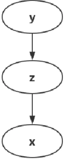
We assume the following data generation process: first a label 𝒚is chosen, aset of latent encoding 𝒛 is generated conditioned on 𝒚. Then data 𝒙 is generated given purely latent encoding

𝒛. Figure 2. shows the probabilistic model of the above generation process.

Figure 3. Probabilistic model for data generation Hence, we have:

𝑝(𝒙, 𝒚, 𝒛) = 𝑝(𝒙|𝒛)𝑝(𝒛|𝒚)𝑝(𝒚)

Similar to VAE. We choose a deep generative network 𝑝_𝜃(𝒙|𝒛; 𝜽) to learn the true probability distribution 𝑝(𝒙|𝒛).

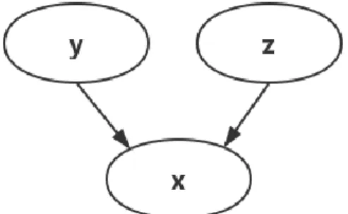
Compared with Berkhahn’s model and Kingma’s M2 model, the proposed generative model removes the direct dependency of data 𝒙 on label 𝒚. Therefore, latent encodings 𝒛have all the information about reconstructing 𝒙. This is a more desirable property for representation learning [3].

Figure 4. Probabilistic model for data generation in Berkhahn’s and Kingma’s work

Inference model

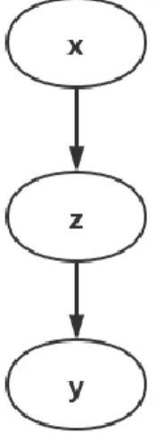
In variation inference setting we use an inference model to approximate posterior distribution 𝑝(𝒛|𝒙, 𝒚) and 𝑝(𝒛, 𝒚|𝒙). Figure 4. describes the inference model. We assume 𝒚can be inferenced by latent encoding𝒛while𝒛can be inferenced directly from 𝒙. Namely, we have:

𝑞_𝜙(𝒙, 𝒚, 𝒛) = 𝑞𝜙(𝒛|𝒙)𝑞𝜙(𝒚|𝒛)𝑞𝜙(𝒙)

Figure 5. Probabilistic model for inference

This is a reasonable assumption because all information about data 𝒙, including

information about label, should be encoded by 𝒛. Therefore, we can infer the label directly from

𝒛. Thissetting also allows us to utilize the nice latent encoding we’ve learnt from generative model for the downstream classification task. We can benefit from the potential disentanglement provided by VAE model.

4.2 Objective function

Similar to Kingma’s work. We also use two different loss function to handle labeled and unlabeled data.

Labeled Data

For labeled data. 𝒚is treated as observed variable. We minimize the following KL term:

𝐾𝐿(𝑞_𝜙(𝒛|𝒙, 𝒚)||𝑝_𝜃(𝒛|𝒙, 𝒚)) = 𝐸_{𝒛~𝑞𝜙(𝒛|𝒙, 𝒚)}log𝑞𝜙(𝒛|𝒙, 𝒚) 𝑝_𝜃(𝒛|𝒙, 𝒚) = 𝐸_{𝒛~𝑞𝜙}(𝒛|𝒙)log

𝑞_𝜙(𝒛|𝒙)𝑝_𝜃(𝒙, 𝒚) 𝑝𝜃(𝒙, 𝒚, 𝒛)

= 𝐸𝒛~𝑞𝜙(𝒛|𝒙)log 𝑞_𝜙(𝒛|𝒙)𝑝_𝜃(𝒙, 𝒚) 𝑝𝜃(𝒙|𝒛)𝑝𝜃(𝒛|𝒚)𝑝𝜃(𝒚) = log 𝑝𝜃(𝒙, 𝒚) − 𝐸𝒛~𝑞𝜙(𝒛|𝒙)log 𝑝𝜃(𝒙|𝒛) − log 𝑝_𝜃(𝑦) +𝐾𝐿(𝑞𝜙(𝒛|𝒙)||𝑝𝜃(𝒛|𝒚)) (15)

Hence, we have the evidence lower bound for labeled data:

ELBOlabeled = log 𝑝𝜃(𝑥, 𝑦) − 𝐾𝐿(𝑞𝜙(𝒛|𝒙, 𝒚)||𝑝𝜃(𝒛|𝒙, 𝒚))

= 𝐸_{𝒛~𝑞𝜙}(𝒛|𝒙)log 𝑝𝜃(𝒙|𝒛) − 𝐾𝐿(𝑞𝜙(𝒛|𝒙)||𝑝𝜃(𝒛|𝒚)) (16)

A classification error 𝐿_𝑐𝑙 = 𝐶𝑟𝑜𝑠𝑠𝐸𝑛𝑡𝑟𝑜𝑝𝑦(𝒛, 𝒚) is also added in order to learn conditional probability 𝑝(𝒚|𝒛).

𝐿(𝒙, 𝒚) = 𝐿_𝑐𝑙− 𝐸𝐿𝐵𝑂_{𝑙𝑎𝑏𝑒𝑙𝑒𝑑} (17)

Unlabeled Data

For unlabeled data. 𝒚is treatedas unobserved latent variable. We minimize:

𝐾𝐿(𝑞_𝜙(𝒛, 𝒚|𝒙)||𝑝_𝜃(𝒛, 𝒚|𝒙)) = 𝐸𝒛~𝑞𝜙(𝒛|𝒙) 𝒚~𝑞𝜙(𝒚|𝒙) log𝑞𝜙(𝒛, 𝒚|𝒙) 𝑝_𝜃(𝒛, 𝒚|𝒙) = 𝐸𝒛~𝑞𝜙(𝒛|𝒙) 𝒚~𝑞𝜙(𝒚|𝒙) log𝑞𝜙(𝒛|𝒙)𝑞𝜙(𝒚|𝒛)𝑝𝜃(𝒙) 𝑝𝜃(𝒙, 𝒚, 𝒛) = 𝐸𝒛~𝑞𝜙(𝒛|𝒙) 𝒚~𝑞𝜙(𝒚|𝒙) log𝑞𝜙(𝒛|𝒙)𝑞𝜙(𝒚|𝒛)𝑝𝜃(𝒙) 𝑝_𝜃(𝒙|𝒛)𝑝𝜃(𝒛|𝒚)𝑝𝜃(𝒚) = log 𝑝𝜃(𝒙) − 𝐸𝒛~𝑞𝜙(𝒛|𝒙)log 𝑝𝜃(𝒙|𝒛) − 𝐸_{𝒚~𝑞𝜙(𝒚|𝒙)}log 𝑝𝜃(𝑦) +𝐸_{𝒚,𝒛~𝑞} 𝜙(𝒚, 𝒛|𝒙)log 𝑞𝜙(𝒚|𝒛) +𝐸_{𝒚~𝑞𝜙(𝒚|𝒛)}𝐾𝐿(𝑞_𝜙(𝒛|𝒙)||𝑝_𝜃(𝒛|𝒚)) (18)

Hence, we have the evidence lower bound for unlabeled data:

−𝐸_{𝒚,𝒛~𝑞𝜙(𝒚, 𝒛|𝒙)}log 𝑞_𝜙(𝒚|𝒛)

−𝐸_{𝒚~𝑞𝜙(𝒚|𝒛)}𝐾𝐿(𝑞_𝜙(𝒛|𝒙)||𝑝_𝜃(𝒛|𝒚)) = −𝑈(𝑥) (19)

Total Loss function

Finally, the total loss function for the entire dataset is now:

𝐿𝑜𝑠𝑠 = ∑ 𝐿(𝑥, 𝑦) (𝑥,𝑦) ∈ 𝑙𝑎𝑏𝑒𝑙𝑒𝑑 + ∑ 𝑈(𝑥) 𝑥 ∈ 𝑢𝑛𝑙𝑎𝑏𝑒𝑙𝑒𝑑 (20) 4.3 Model architecture

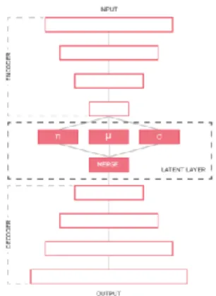
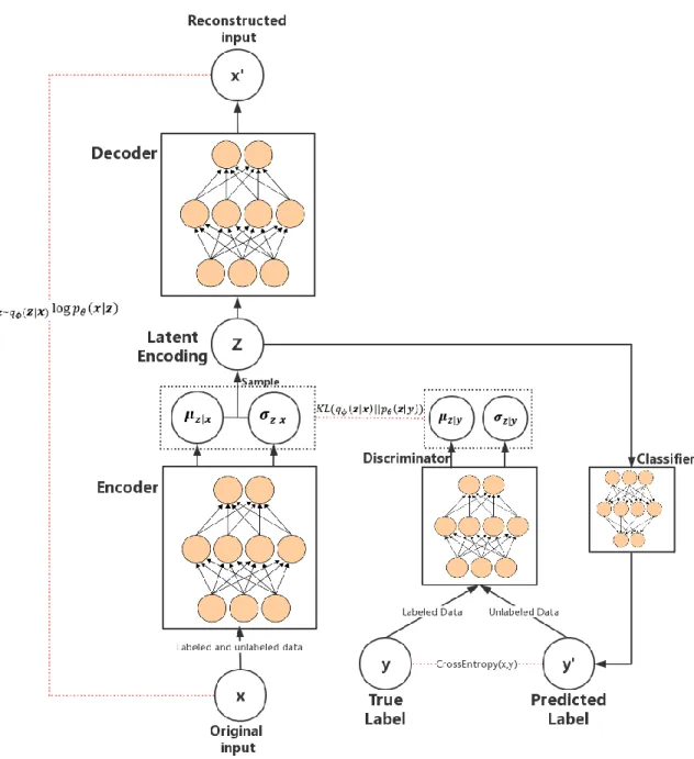
As is shown in Figure 5. Our model is a modified version of vanilla

variational-autoencoder. In order to optimize (16) and (19), some addition structures are added, including a classify-layer that outputs conditional probability 𝑞_𝜙(𝒚|𝒛) and predicts label 𝒚′, and a

discriminator taking 𝒚 or 𝒚′ as input and outputs 𝝁𝒛|𝒚 and 𝝈𝒛|𝒚.

When a labeled input 𝒙_𝒍is fed to the model. The classify-layer tries to learn 𝑝(𝒚|𝒛) by minimizing cross entropy loss. The true label 𝒚is fed to discriminator therefore

𝐾𝐿(𝑞𝜙(𝒛|𝒙)||𝑝𝜃(𝒛|𝒚)) is then computed.

When an unlabeled input 𝒙_𝒖is fed to the model. The classify-layer outputs probability

𝑞_𝜙(𝒚|𝒛). Then predicted label 𝒚′is fed to the discriminator so that

𝐸_{𝒚~𝑞𝜙(𝒚|𝒛)}𝐾𝐿(𝑞_𝜙(𝒛|𝒙)||𝑝_𝜃(𝒛|𝒚)) is computed.

For both labeled and unlabeled data. Reconstruction error is computed, which is equivalent to term 𝐸_{𝒛~𝑞𝜙}(𝒛|𝒙)log 𝑝𝜃(𝒙|𝒛).

CHAPTER 5. EXPERIMENTS

In this chapter, we show an empirical evaluation of the proposed model, referred to as SSLGM (Semi-Supervised Learning with Generative Model) in this report. We show that the proposed model effective in Semi-Supervised learning, as well as competitive comparing with other related works. Open source code, together with most important figures and results, is available at: https://github.com/Fuu3214/SSLGM.git.

5.1 Experiment Setup Dataset

We use the well-known MNIST hand written digit dataset for experiment. The data set for semi-supervised learning is created by randomly splitting 60000 training data into labeled and unlabeled set. The size of labeled data is chosen to be 100, 600 and 1000 separately.

Model Setup

We experiment with two SSLGM models. The first model consists of shallow MLP encoder and decoder, with 10-dimensional latent variable 𝒛. The secondmodel uses more complex Convolutional Neural networks as encoder and decoder, with 50-dimensional latent variable. Table 1 shows the detail for two models.

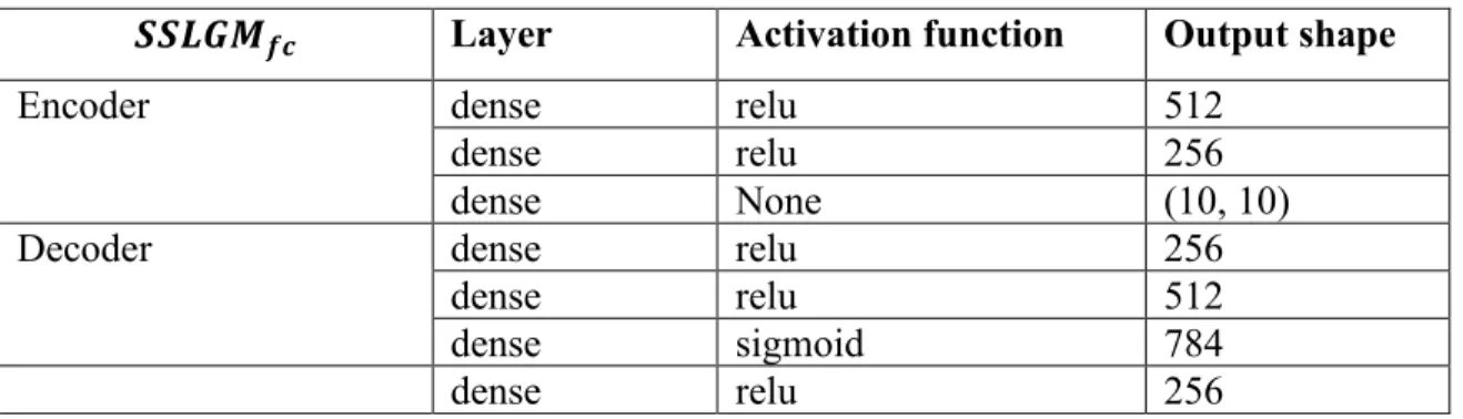
Table 1. 𝑆𝑆𝐿𝐺𝑀_𝑓𝑐 model structure

𝑺𝑺𝑳𝑮𝑴_𝒇𝒄 Layer Activation function Output shape

Encoder dense relu 512

dense relu 256

dense None (10, 10)

Decoder dense relu 256

dense relu 512

dense sigmoid 784

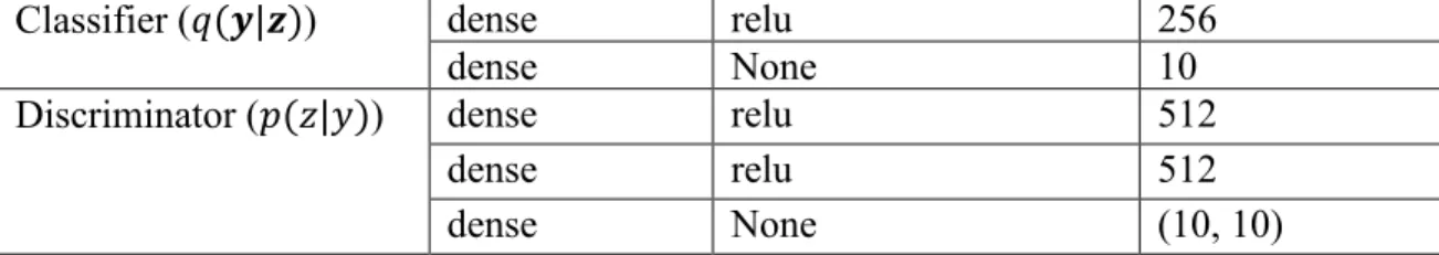
Classifier (𝑞(𝒚|𝒛)) dense relu 256

dense None 10

Discriminator (𝑝(𝑧|𝑦)) dense relu 512

dense relu 512

dense None (10, 10)

Table 2. 𝑆𝑆𝐿𝐺𝑀_𝑐𝑛𝑛 model structure

𝑺𝑺𝑳𝑮𝑴_𝒄𝒏𝒏 Layer Activation

function

Number of filters

Encoder 3 × 3 convolutional relu 32 max_pooling2d 3 × 3 convolutional relu 64 max_pooling2d 3 × 3 convolutional relu 32 max_pooling2d dense None (30, 30)

Decoder dense relu 256

dense relu 512

dense sigmoid 784

Classifier (𝑞(𝒚|𝒛)) dense relu 256

dense relu 256

dense None 30

Discriminator (𝑝(𝑧|𝑦)) dense relu 512

dense relu 512

dense None (30, 30)

5.2 Semi-supervised learning performance 5.2.1 Benchmarking

For benchmarking, we compare our model with supervised models such as fully

connected neural work and convolutional neural network trained on labeled data only, as well as related semi-supervised learning models such as Kingma’s M1 and M2 model and Berkhahn et

Result

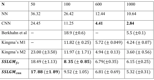
Table 3 shows the benchmarking result. Given fewer labeled examples, both of our models perform better than other models, including purely supervised models as well as semi-supervised models, demonstrating the effectiveness of latent representation learnt by VAE on the downstream classification tasks. However, when number of labels becomes larger, the power of CNN on image classification tasks becomes more significant. It performs better compared with all semi-supervised learning models.

Comparing two of our models 𝑺𝑺𝑳𝑮𝑴_𝒇𝒄and𝑺𝑺𝑳𝑮𝑴_𝒄𝒏𝒏. 𝑺𝑺𝑳𝑮𝑴_𝒄𝒏𝒏performs slightly better than 𝑺𝑺𝑳𝑮𝑴_𝒇𝒄 thanks to the power of CNN on extracting image features as well as preventing from overfitting.

Table 3. Semi-supervised MNIST classification results

N 50 100 600 1000 NN 36.32 26.42 12.44 10.64 CNN 24.45 11.25 4.41 2.84 Berkhahn et al − 18.9 (±0.6) − 5.5 (±0.1) Kingma’s M1 − 11.82 (± 0.25) 5.72 (± 0.049) 4.24 (± 0.07) Kingma’s M2 23.00 (±3.50) 11.97 (± 1.71) 4.94 (± 0.13) 3.60 (± 0.56) 𝑺𝑺𝑳𝑮𝑴_𝒇𝒄 18.49 (±1.13) 𝟖. 𝟑𝟓 (± 𝟎. 𝟖𝟓) 6.79(±0.35) 6.15 (±0.25) 𝑺𝑺𝑳𝑮𝑴𝒄𝒏𝒏 𝟏𝟕. 𝟖𝟖 (±𝟏. 𝟖𝟗) 9.52 (± 1.05) 6.81 (± 0.69) 5.32 (±0.31)

5.2.2 The effect of unlabeled data

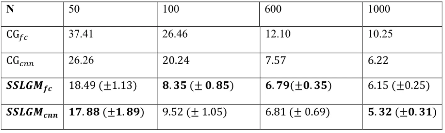
We show that unlabeled data improves classification performance in our model. We compare our model with control groups CG_𝑓𝑐 and CG_𝑐𝑛𝑛. The control group models are obtained by first removing the unsupervised components and then train the model only on labeled data. We choose exactly the same hyper-parameters, including number of hidden units, dimension of latent variables, number of layers of MLP and number of filters for CNN. We use classification error rate on testing dataset as our evaluation metric.

Result

The result in Table 4 shows that, in our model setting, unlabeled data is extremely helpful in improving semi-supervised classification performance, especially when we are given less labeled data. We also observe that, without unlabeled data, both of the control group models tend to overfit after a small number of training epochs. However, 𝑺𝑺𝑳𝑮𝑴_𝒇𝒄and𝑺𝑺𝑳𝑮𝑴_𝒄𝒏𝒏hardly overfit even after a few hundred epochs. This shows that unlabeled data serves as a regularizer to the model.

Table 4. MNIST classification results compared with control groups

N 50 100 600 1000

CG𝑓𝑐 37.41 26.46 12.10 10.25

CG_𝑐𝑛𝑛 26.26 20.24 7.57 6.22

𝑺𝑺𝑳𝑮𝑴_𝒇𝒄 18.49 (±1.13) 𝟖. 𝟑𝟓 (± 𝟎. 𝟖𝟓) 𝟔. 𝟕𝟗(±𝟎. 𝟑𝟓) 6.15 (±0.25) 𝑺𝑺𝑳𝑮𝑴𝒄𝒏𝒏 𝟏𝟕. 𝟖𝟖 (±𝟏. 𝟖𝟗) 9.52 (± 1.05) 6.81 (± 0.69) 𝟓. 𝟑𝟐 (±𝟎. 𝟑𝟏)

5.3 Conditional data generation 5.3.1 Style and content separation

To demonstrate that model is capable of learning useful latent representation with a small number of labeled data. We use the decoder of 𝑺𝑺𝑳𝑮𝑴_𝒇𝒄model trained on 100 labeled data. In the first experiment we examine the style and content separation. First, we first randomly pick a class label and feed it to discriminator to acquire (𝝁_𝒛|𝒚, 𝝈_𝒛|𝒚). Then we randomly select two dimensions [𝑧_𝑎, 𝑧_𝑏] of the latent encoding 𝒛and we range them as follow:

𝑧_𝑎 = 𝑃𝑃𝐹_𝑁(𝜇 𝑧|𝑦 𝑎 _,𝜎 𝑧|𝑦𝑎 )(𝛼) 𝑧𝑏 = 𝑃𝑃𝐹_𝑁(𝜇 𝑧|𝑦 𝑏 _,𝜎 𝑧|𝑦𝑏 )(𝛽) (20)

Where 𝑃𝑃𝐹 is the Percent Point Function and 𝛼 and 𝛽 are evenly spaced numbers over

[0.05, 0.95].

For other dimensions we simply sample each of them from gaussian distribution

𝑧𝑖~𝑁(𝜇𝑧|𝑦𝑖 , 𝜎𝑧|𝑦𝑖 ) once and then fix them. This guarantees that only two dimensions changes. To

generate MNIST examples we simply feed 𝒛 to the decoder.

Result

In Figure 7 we choose dimension (𝑧₀, 𝑧₁) and generate 3 sets of digits from label 2,3,7. We see that as 𝑧₀ becomes larger, the width of digit tends to becomes smaller, while as 𝑧₁

becomes larger the digit tends to becomes more rounded. In Figure 8 we choose dimension

(𝑧₀, 𝑧₅) and generate digits from label 0, 5. We observe that as 𝑧₀ becomes larger, the width of digit also becomes smaller, while as 𝑧₅ becomes larger, the angle of digits change.

Figure 7. Conditional generation by fixing other dimensions while varying 𝑧₀, 𝑧₁

Figure 8. Conditional generation by fixing other dimensions while varying 𝑧₀, 𝑧₅

5.3.2 Conditional data generation performance

In the second experiment we use the decoder of 𝑺𝑺𝑳𝑮𝑴_𝒇𝒄model trained on 100 labeled data to evaluate the conditional generation performance. To generate data, we simply sample 𝒛

Result

Figure 9 demonstrate an example of conditional data generation performance of our

𝑺𝑺𝑳𝑮𝑴_𝒇𝒄model trained on 100 labeled data. Our model creates more accurate and more diverse data conditional on the label compared with Kingma’s M2 model shown in Figure 10.

Figure 9. Conditional data generation performance of 𝑺𝑺𝑳𝑮𝑴𝒇𝒄. Data is generated conditioned

on label 0, 5, 6 respectively.

Figure 10. Conditional data generation performance of Kingma’s M2 model. Data is generated conditioned on label 0, 5, 6 respectively.

CHAPTER 6. CONCLUSION

We propose a new semi-supervised generative model to overcome a drawback of existing approaches. We remove the direct dependency of data generation on label. Compared with related works that directly concatenate latent encoding with label, our new approach improves quality of latent representations. Moreover, unlike existing works, our approach is capable of utilizing the nice latent representations obtained by variational autoencoder in the downstream classification tasks. Experiments also demonstrate the efficiency of our approach with respect to semi-supervised learning performance and conditional data generation given a relatively small number of labeled data.

One drawback of our model is overfitting. In some scenario such as few-shot or one-shot learning, the number of labeled data is extremely small. In these situations, the performance of our model will drop sharply. This is because the supervised component is overfitting while unsupervised component is still underfitting. Given unlabeled data, classifier gives wrong predictions frequently and influence conditional generation, hence impacts the quality of latent representation. We observe the same problem in other existing semi-supervised generative models as well. By adopting methods such as adding dropout layer and batch normalization, our model partially overcome this problem. But further investigation is still needed to improve performance on fewer labeled data. This can be a direction for our future work. Another potential direction for future work is applying our model in other domains. For example, text image

transformation, where image is generated conditioned on text information obtained by some NLP models.

REFERENCES

[1] D. P. Kingma, S. Mohamed, D. J. Rezende, and M. Welling, “Semi-supervised learning with

deep generative models,” in Advances in neural information processing systems, 2014, pp. 3581–3589.

[2] F. Berkhahn, R. Keys, W. Ouertani, N. Shetty, and D. Geißler, “One model to rule them all,”

arXiv preprint arXiv:1908.03015, 2019.

[3] Y. Bengio, A. Courville, and P. Vincent, “Representation learning: A review and new

perspectives,” IEEE transactions on pattern analysis and machine intelligence, vol. 35, no. 8, pp.

1798–1828, 2013.

[4] D. M. Blei, A. Kucukelbir, and J. D. McAuliffe, “Variational inference: A review for statisticians,” Journal of the American Statistical Association, vol. 112, no. 518, pp. 859–877, 2017.

[5] D. P. Kingma and M. Welling, “Auto-encoding variational bayes,” arXiv preprint

arXiv:1312.6114, 2013.

[6] Y. Cheng, “Semi-supervised learning for neural machine translation,” in Joint Training for Neural Machine Translation. Springer, 2019, pp. 25–40.

[7] Y.-A. Chung, Y. Wang, W.-N. Hsu, Y. Zhang, and R. Skerry-Ryan, “Semi-supervised training for improving data efficiency in end-to-end speech synthesis,” in ICASSP 2019-2019 IEEE International Conference on Acoustics, Speech and Signal Processing (ICASSP). IEEE, 2019, pp. 6940–6944.

[8] R. Fergus, Y. Weiss, and A. Torralba, “Semi-supervised learning in gigantic image

collections,” in Advances in neural information processing systems, 2009, pp. 522–530.

[9] M. Shi and B. Zhang, “Semi-supervised learning improves gene expression-based prediction

of cancer recurrence,” Bioinformatics, vol. 27, no. 21, pp. 3017–3023, 2011.

[10] R. Johnson and T. Zhang, “Semi-supervised convolutional neural networks for text

categorization via region embedding,” in Advances in neural information processing systems,