1
Two-level survival analysis models
The dataThe data set for this example is taken from Schoenwald & Henggeler (2005). Children in the study were assigned to therapists and followed across time. At the child level, data were collected at baseline (pre-treatment,T0), post-treatment (T1), 6 months post-treatment (T2), and 12 months post- treatment (T3). The outcome of interest is whether a child was suspended in the current school year, assessed at T0, T1, T2,or T3. Specifically, here, we will focus on the time until the first school suspension as the "survival" outcome. As indicated in more detail later, this is indicated by a combination of the variables Event and Suspend: for example, if the student was suspended, the indicator Event is given the value 1 and Suspend will indicate the
time period during which this occurred. However, there are also subjects who do not experience the event (i.e., were not suspended), and who drop out of the study before its end. Such subjects are considered to be right-censored in the survival analysis literature, and for these subjects the Event variable is coded 0 and the Suspend variable indicated the last time
period prior to their dropout from the study. For subjects who never experience the event and who never drop out, they receive Event codes of 0 and Suspend codes equal to the final time
point. In addition to these data concerning school suspension, the gender of each student was also recorded, as well as whether or not the student's family was receiving financial assistance. The first 8 cases of the data set suspend.ss3 are shown below.
2
The variables of interest are:
o Therapst is the patient therapist ID (443 level-2 units).
o YouthID is the child's ID (1914 level-1 units).
o Suspend is an ordinal outcome variable that assumes values 1, 2, 3 or 4, corresponding
to the time points T0, T1, T2,and T3.
o Event is the event indicator, where 1 indicates suspension took place and 0 that the
observation was censored.
o SexF indicates the child's gender (1 = female; 0 = male).
o FinnAsst equals 1 if financial assistance is given to the student's family and 0 otherwise
o SexFin equals SexF × FinnAsst and therefore assumes values of 0 and 1. The model
Let yij denote an ordinal outcome variable that takes on discrete positive values t=1,2, , . m In previous examples we assumed that yij has C categories. For example
• 1 = not depressed, • 2 = mildly depressed, • 3 = depressed and • 4 = extremely depressed.
The subscript ( , )i j denotes subject j, j=1,2,ni nested within level-2 unit i, i=1,2, , N . In the present context the level-1 units j indicates children and the level-2 unit i indicates therapists. Note, that as another example of this type of model, one could have multiple failure times nested within individuals.
3
Let δij denote the censor/event indicator, then δij =1 if the event occurs and δij =0 if an observation is censored. In survival analysis each ij is observed until time tij and if an event occurs tij =t and δij =1. If the observation is censored at tij =t then δij =0.
In the case of censoring it is assumed that a unit is observed at tij but not at tij+1. Hedeker,
Siddiqui & Hu (2000) showed that if events occur within continuous time intervals (i.e., grouped-time), for example, a student is suspended in the past year, use of the complementary log-log link for an ordinal outcome is equivalent to a proportional hazards model in continuous time. Therefore, the grouped-time proportional hazards mixed model can be written as:
( )
(
)
log log 1− −P tij = +γt w′ijα x β+ ′ij i
where wij is a vector of explanatory variables and xij a vector of fixed effects. Typically, the elements of xij are a subset of wij. For example, the elements of xij might correspond to the intercept and age, whereas wij would include these two terms plus any additional model covariates. It is assumed that the random effects βi are from a normal distribution with mean zero and covariance matrix Φ.
( )
ijP t denotes the probability that an event takes place in the interval designated at time tij. t
γ represent threshold values, and in the present context these reflect the baseline hazard (i.e., the hazard when all covariates equal 0). The plus sign following γt means that a positive α indicates an increased hazard (i.e., the event occurs sooner) as values of the covariate increase. Survival data as ordinal outcomes
Assume 4 time points with no intermittent censoring and let y denote the outcome variable. Let us first consider subjects who were suspended at some point in the study. For these subjects, the variable Event will be coded as 1 and the coding of the Suspend variable will be as follows. Suspend:
1:
ij
y = Student first suspended at T0. 2 :
ij
y = Student not suspended at T0, but first suspended at T1. 3:
ij
4 4 :
ij
y = Student not suspended at T0, T1 or T2 , but first suspended at T3.
Similarly, subjects who were never censored would have the variable Event coded as 0, and the following codes for the Suspend variable.
Suspend: 1:
ij
y = Student not suspended at T0 and no data beyond T0. 2 :
ij
y = Student not suspended at T0or T1 , and no data beyond T1. 3:
ij
y = Student not suspended at T0,T1 , or T2 , and no data beyond T2(i.e., no data at T3
). 4 :
ij
y = Student not suspended at T0, T1 , T2 , or T3.
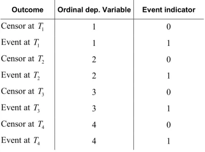
Table 3.10 shows how values are assigned to yij, and the relationship between the yij outcomes and the event indicator.
Table 3.10: Four time points with censoring
Outcome Ordinal dep. Variable Event indicator
Censor at T1 1 0 Event at T1 1 1 Censor at T2 2 0 Event at T2 2 1 Censor at T3 3 0 Event at T3 3 1 Censor at T4 4 0 Event at T4 4 1
It should be noted that one could also fit grouped-time survival models using dichotomous indicators of event/censoring across the study time points. This approach, which is described in Singer and Willett (1993), can also be done in SuperMix, though additional data setup and
5
manipulation is required. The advantage of representing the survival data as ordinal outcomes is that there is no need to include time indicators since the thresholds take care of this. The ordinal presentation is also more efficient in terms of data set size, especially when the number of time points is large. More information on these two different approaches can be found in Hedeker, Siddiqui & Hu (2000).
Example
The model is fitted to the data in suspend.ss3as follows. The first step is to create the ss3 file shown above from the Excel file suspend.xls. This is accomplished as follows:
o Use the Import Data File option on the File menu to load the Open dialog box.
o Browse for the file suspend.xls in the Examples, Survival folder.
o Select the file and click on the Open button to open the following SuperMix spreadsheet
window for suspend.ss3.
Setting up the analysis
We start by selecting the New Model Setup option on the Filemenu to load the Model Setup window.
6
First, enter the titles Survival Analysis Using Ordered Responses and Complementary log-log link function in the Title 1 and Title 2 text boxes respectively. Select the ordinal outcome variable Suspend from the Dependent Variabledrop-down list box. The variable Therapst, which defines
the levels of the hierarchy, is selected as the Level-2 ID from the Level-2 IDs drop-down list box.
Also set the number of iterations to 50.
Next, click on the Variables tab of the Model Setup window. SexF, FinnAsst, andSexFin are
specified as the predictors (explanatory variables) of the fixed part of the model by checking the corresponding boxes in the E column of the Available grid on the Variables screen. These actions will produce the following screen.
7
To specify the number of quadrature points and link function (Function Model), we proceed to the Advanced screen by clicking on the Advanced tab. Change Model Terms from subtract to add and select complementary log-log as the Function Model. Select non-adaptive quadrature as Optimization Method, and request 25 quadrature points. Finally, set the Right-censoring field to include,
and select the variable Event as Censor Variable.
To complete the model setup, we will illustrate use of the Linear Transforms option. In the current model specification, the baseline hazard is a function of the model intercept and thresholds. Specifically, the baseline hazard estimate at the first time point equals the estimated model intercept, the baseline hazard estimate at the second time point is the sum of the model intercept and the first estimated threshold, the baseline hazard at the third time point is the sum of the model intercept and the second estimated threshold, and the baseline hazard estimate at the final time point is a sum of the estimated intercept and the third estimated threshold. Thus, three of these baseline hazard estimates involve sums of the estimated parameters. To obtain these linear transforms of the model estimates, click on the Linear Transforms tab. The three linear transforms are specified as follows:
Intercpt SexF FinnAsst SexFin Random Intercpt (L-2)
Threshold 1 Threshold 2 Threshold 3
1 0 0 0 0 1 0 0
1 0 0 0 0 0 1 0
1 0 0 0 0 0 0 1
8
For the second transform, values of 0, 1, 0 are assigned for the thresholds. The third transform contains values of 0, 0, 1 for the three thresholds. This step completes the model set-up. Use the File, Save option to save the model setup to a file named suspend1.mum. Next, use the Analysis, Run option on the main menu bar to run the analysis.
Discussion of results
The portion of the output file shown below indicates that there are 443 therapists. Nested within these level-2 units are 1914 subjects. A summary of the number of level-1 observations per level-2 unit (only first two lines shown) is also given.
9
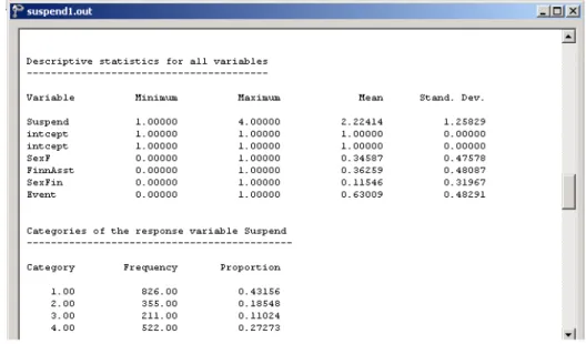
This part of the output is followed by descriptive statistics for all the variables. The variable
Suspend has four categories with values 1, 2, 3 and 4. Except for the intercept term, the
remaining variables are all dichotomous.
The proportions of subjects assigned a value of 1, 2, 3 or 4 are 0.432, 0.185, 0.110 and 0.273 respectively. A crosstabulation of Suspend by Event is given in Table 3.11. It follows that, for
example, 773 students out of the 1914 in the study were suspended prior to treatment (T0). For 53 children, we only know that they were not suspended at T0, thereafter they are missing and treated as right-censored.
Table 3.11: Crosstabulation of Suspend by Event
0
T T1 T2 T3
773 255 106 72
53 100 105 450
Parameter estimates are given in the next part of the output. We conclude that there is no gender-financial assistance interaction and that all the remaining parameter estimates are significant. The effect of SexF is negative indicating that girls have a significantly decreased hazard (i.e., a longer
time to the first suspension), relative to boys. The FinnAsst estimate is positive indicating an
increased hazard (shorter time to first suspension) for children from families receiving financial assistance, relative to children from families not receiving this assistance.
10
The last part of the output contains an estimate of the intracluster correlation. Although this estimate indicates a modest therapist effect, the random effect variance term is highly significant. From this we conclude that the time until suspension does vary significantly across therapists.
11
A summary of the transforms (given in transposed form) is given followed by a significance test for each transform. In combination with the intercept estimate, these provide the estimates of the baseline hazard (i.e., the hazard when all covariates equal 0). Specifically, the baseline hazard estimates for the four study time points are -0.65649, -0.22377, -0.03265, and 0.12110. These can be converted to the probability scale using the inverse of the complementary log-log function, namely,
( ) 1 exp[ exp( )]
P z = − − z
This yields probability estimates of the baseline hazard for the first school suspension as .405, .550, .620, and .677 across these four study time points. Note that these are conditional estimates, conditional on the therapist effects. In other words, they are estimates controlling for the effect of therapist on the individual student outcomes.