ORNA AGMON BEN-YEHUDA, MULI BEN-YEHUDA,
ASSAF SCHUSTER and DAN TSAFRIR, Technion – Israel Institute of Technology
Cloud providers possessing large quantities of spare capacity must either incentivize clients to purchase it or suffer losses. Amazon is the first cloud provider to address this challenge, by allowing clients to bid on spare capacity and by granting resources to bidders while their bids exceed a periodically changing spot price. Amazon publicizes the spot price but does not disclose how it is determined.
By analyzing the spot price histories of Amazon’s EC2 cloud, we reverse engineer how prices are set and construct a model that generates prices consistent with existing price traces. Our findings suggest that usually prices are not market-driven, as sometimes previously assumed. Rather, they are likely to be generated most of the time at random from within a tight price range via a dynamic hidden reserve price mechanism. Our model could help clients make informed bids, cloud providers design profitable systems, and researchers design pricing algorithms.
Categories and Subject Descriptors: G.3 [Probability and Statistics]: Time Series Analysis General Terms: Economics, Design
Additional Key Words and Phrases: Amazon EC2, reverse engineering, spot instances ACM Reference Format:
Agmon Ben-Yehuda, O., Ben-Yehuda, M., Schuster, A., and Tsafrir, D., T. F. 2012. Deconstructing Amazon EC2 Spot Instance Pricing. ACM Trans. Econ. Comp. V, N, Article A (January YYYY), 21 pages.
DOI=10.1145/0000000.0000000 http://doi.acm.org/10.1145/0000000.0000000 1. INTRODUCTION
Unsold cloud capacity is wasted capacity, so cloud providers would naturally like to sell it. They would especially like to sell the capacity of machines which cannot be turned off and have higher overhead expenses. Clients might be enticed to purchase this capacity if they are provided with enough incentive, notably, a cheaper price. In late 2009, Amazon was the first cloud provider to attempt to provide such an incentive by announcing itsspot instancespricing system. “Spot Instances [...] allow customers to bid on unused Amazon EC2 capacity and run those instances for as long as their bid exceeds the current Spot Price. The Spot Price changes periodically based on supply and demand, and customers whose bids exceeds it gain access to the available Spot Instances” [Amazon 2009]. With this system, Amazon motivates purchasing cheaper capacity while ensuring it can continuously act in its best interest by maintaining control over the spot price.Section 2summarizes the publicly available information regarding Amazon’s pricing system.
A preliminary version of this work, which did not utilize cloud workload traces, appeared in IEEE CloudCom 2011 [Agmon Ben-Yehuda et al. 2011].
This work was partially supported by the Technion Hasso Plattner Center.
Authors’ addresses: O. Agmon Ben-Yehuda and M. Ben-Yehuda and A. Schuster and D. Tsafrir, Computer Science Department, Technion – Israel Institute of Technology, Haifa, Israel. {ladypine, muli, assaf, dan}@cs.technion.ac.il.
Permission to make digital or hard copies of part or all of this work for personal or classroom use is granted without fee provided that copies are not made or distributed for profit or commercial advantage and that copies show this notice on the first page or initial screen of a display along with the full citation. Copyrights for components of this work owned by others than ACM must be honored. Abstracting with credit is per-mitted. To copy otherwise, to republish, to post on servers, to redistribute to lists, or to use any component of this work in other works requires prior specific permission and/or a fee. Permissions may be requested from Publications Dept., ACM, Inc., 2 Penn Plaza, Suite 701, New York, NY 10121-0701 USA, fax+1 (212) 869-0481, or [email protected].
c
YYYY ACM 1946-6227/YYYY/01-ARTA $15.00
Amazon does not disclose its underlying pricing policies. Despite much interest from outside Amazon [Chohan et al. 2010; Samovskiy 2011; Mattess et al. 2010; Wee 2011; Javadi and Buyya 2011], its spot pricing scheme has not, until now, been deciphered. The only information Amazon does reveal is its temporal spot prices, which must be publicized to make the pricing system work. While Amazon provides only its most re-cent price history, interested parties record and accumulate all the data ever published by Amazon, making it available on the Web [Lossen 2010; Vermeersch 2010]. We lever-age the resulting trace files for this study. The trace files, along with the methodology we employ to use them, are described inSection 3.
Knowing how a leading cloud provider like Amazon prices its unused capacity is of potential interest to both cloud providers and cloud clients. Understanding the con-siderations, policies, and mechanisms involved may allow other providers to better compete and to utilize their own unused capacity more effectively. Clients can likewise exploit this knowledge to optimize their bids, to predict how long their spot instances would be able to run, and to reason about when to purchase cheaper or costlier capac-ity.
Motivated by these benefits, we attempt in Sections 4–5 to uncover how Ama-zon prices its unused EC2 capacity. We construct a spare capacity pricing model and present evidence suggesting that prices are typicallynotdetermined according to Ama-zon’s public definition of the spot pricing system as quoted above. Rather, the evidence suggests that spot prices are usually drawn from a tight, fixed range of prices, reflect-ing a random reserve price that is not driven by supply and demand. (Areserve price
is a hidden price below which bids are ignored.) Consequently, published spot prices reveal little about actual, real-life client bids; studies that assume otherwise (in par-ticular [Zhang et al. 2011; Chen et al. 2011]) are, in our view, misguided.We speculate that Amazon utilizes such a price range because its spare capacity usually exceeds the demand.
InSection 6we put our model to the test by conducting pricing simulations (based on cloud and grid workloads) and by showing their results to be consistent with EC2 price traces. We then discuss the possible benefits of using dynamic reserve price sys-tems (such as the one we believe is used by Amazon) inSection 7. Finally, we survey the related work inSection 8and offer some concluding remarks inSection 9.
2. PRICING CLOUD INSTANCES
Amazon’s EC2 clients rent virtual machines calledinstances, such that each instance has a type describing its computational resources as follows: m1.small, m1.large and m1.xlarge denote, respectively, small, large, and extra-large “standard” instances; m2.xlarge,m2.2xlarge, and m2.4xlargedenote, respectively, large, double extra-large, and quadruple extra-large “high memory” instances; and c1.medium and c1.xlargedenote, respectively, medium and extra-large “high CPU” instances.
An instance is rented within a geographical region. We use data from four EC2 re-gions: us-east,us-west,eu-westandap-southeast, which correspond to Amazon’s data centers in Virginia, California, Ireland, and Singapore.
Amazon offers three purchasing models, all requiring a fee from a few cents to a few dollars, per hour, per running instance. The models provide different assurances regarding when instances can be launched and terminated. Paying a yearly fee (of hun-dreds to thousands of dollars) buys clients the ability to launch onereserved instance
whenever they wish. Clients may instead choose to forgo the yearly fee and attempt to purchase an on-demand instancewhen they need it, at a higher hourly fee and with no guarantee that launching will be possible at any given time. Both reserved and on-demand instances remain active until terminated by the client.
launch or termination time. When placing a request for a spot instance, clients bid the maximum hourly price they are willing to pay for running it (calleddeclared price
or bid). The request is granted if the bid is higher than the spot price; otherwise it waits. Periodically, Amazon publishes a new spot price and launches all waiting in-stance requests with a maximum price exceeding this value; the inin-stances will run until clients terminate them or the spot price increases above their maximum price. All running spot instances incur a uniform hourly charge, which is the current spot price. The charge is in full hours, unless the instance was terminated due to a spot price change, in which case the last fraction of an hour is free of charge.
In this work, we assume that instances with bids equal to the spot price are treated similarly to instances with bids higher than the spot price.
3. METHODOLOGY
Trace Files.We analyze 64 (= 8×4×2) spot price trace files associated with the 8 aforementioned instance types, the 4 aforementioned regions, and 2 operating sys-tems (Linux and Windows). The traces were collected by Lossen [Lossen 2010] and Vermeersch [Vermeersch 2010]. They start as early as 30 November 2009 (traces for regionap-southeastare only available from the end of April 2010). In this paper, unless otherwise stated, we use data accumulated until 13 July 2010.
Availability. We define the availability of a declared price as the fraction of the time in which the spot price was equal to or lower than that declared price. Formally, a per-sistent requestis a series of requests for an instance that is immediately re-requested every time it is terminated due to the spot price rising above its bid. Given a declared priceD, we define D’savailability to be the time fraction in which a persistently re-quested instance would run ifD is its declared price. Formally, letH be a spot price trace file, and letTbandTebe the beginning and end of a time interval withinH. The
availability ofDwithinHduring[Tb, Te]is:
availabilityH(D)|[Tb,Te]= TH
b→e(D)
Te−Tb
, whereTbH→e(D)denotes the time betweenTb andTeduring which the spot price was
lower than or equal toD. The availability of priceD reflects the probability that spot instances with this bid would be immediately launched when requested at some uni-formly random time within[Tb, Te].
4. EVIDENCE FOR ARTIFICIAL PRICING INTERVENTION 4.1. Market-Driven Auctions
Amazon’s description of “How Spot Instances Work” [Amazon 2009] gives the impres-sion that spot prices are set through a uniform price, sealed-bid, market-driven auc-tion. “Uniform price” means all bidders pay the same price. “Sealed-bid” means bids are unknown to other bidders. “Market-driven” means the spot price is set according to the clients’ bids. Many auctions fit this description. One example of such an auction is an(N+ 1)thprice auction of multiple goods, with retroactive supply limitation (after
clients bid). Of course, Amazon could be using some other market-driven mechanism consistent with their description.
In an(N + 1)th price auction of multiple goods, each client bids for a single good
(i.e., a spot instance). The provider sorts the bids and chooses the topN bidders. The provider is free to set the number of sold goods N, as long asN does not exceed the available capacity. The provider may set N up-front as the available capacity, but it may also retroactively further restrictNafter receiving the bids, to maximize revenue.
0.5 1 1.5 2 2.5 0 0.2 0.4 0.6 0.8 1 availability
declared price [$/hour]
us−east m1 instances us−east m2.xlarge instance us−east m2 2xlarge and 4xlarge us−east c1 instances other regions m1 instances other regions m2.xlarge instances
other regions m2 2xlarge and 4xlarge instances other regions c1 instances
Floor Price (F)
Knee at Ceiling Price (C)
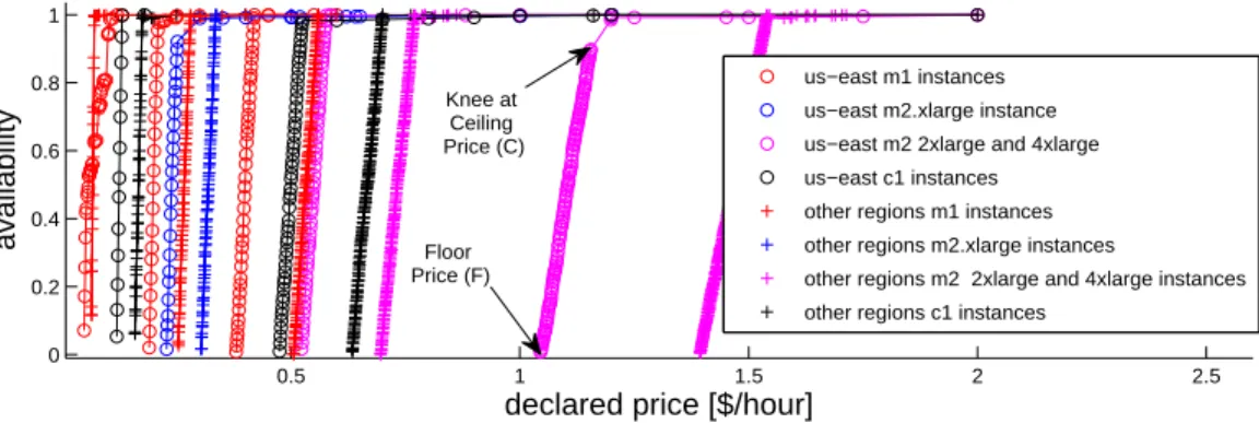
Fig. 1. Availability of Windows-running spot instance types as a function of their declared price. The legend is multiplexed:us-west,eu-west,ap-southeastall appear in the legend as “other regions”.m1.small,m1.large andm1.xlargeall appear asm1.c1.mediumandc1.xlargeappear asc1.
The provider sets the uniform price to the price declared by the highest bidder whodid notwin the auction (bidder numberN+ 1) and publishes it. The topNwinning bidders pay the published price and their instances start running. In this case, the published price is a price bid by an actual client.
The provider may also decide to ignore bids below a hiddenreserve priceor below a publicly knownminimal price, to prevent the goods from being sold cheaply, or to give the impression of increased demand.
We conjecture that usually, contrary to impressions conveyed by Amazon [Amazon 2009] and assumptions made by researchers [Zhang et al. 2011; Chen et al. 2011], the spot price is set according to a constantly changing reserve price, disregarding client bids. In other words, most of the time the spot price isnotmarket-driven but is set by Amazon according to an undisclosed algorithm.
4.2. Evidence: Availability as a Function of Price
In support of this conjecture, we analyze the relationship between an instance’s de-clared price (how much a client would be willing to pay for it) and the resulting avail-ability between 20 January 2010 and 13 July 2010. Fig. 1 shows the availavail-ability of different spot instance types as a function of declared price (price-availability graphs), for all examined Windows spot instance types in all regions. Results for instances run-ning Linux (not shown) are qualitatively similar. The prices of different resources are usually in different ranges (e.g.,us-east.c1.medium’s usual price range is a third of us-east.c1.xlarge’s), but they all share the same functional shape: a sharp linear increase in availability, during which the price resolution is 0.1 cent. The increase may last un-til an availability of 1.0 is reached, or end with a kneeat a high availability (usually above 0.95). A knee is a sharp change in the graph’s slope; it is usually accompanied by a sharp decrease in the graph’s resolution. Above the knee, the availability grows with declared price, but at a slower, varying rate.
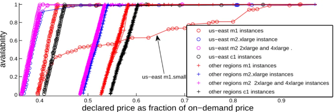
Fig. 2 shows normalized price-availability graphs for Linux: each spot price is di-vided by the price of a similar on-demand instance. We see that Linux types can be classified by region. Each of the two region classes has a distinct normalized price range in which the availability’s dependency on the price is linear. One class contains us-east, and the other class contains the other regions.
Fig. 3 shows the data presented in Fig. 1 as normalized price-availability graphs. As in Fig. 2, different types can be classified by region: us-eastor all other regions. Not
0.3 0.35 0.4 0.45 0.5 0.55 0.6 0.65 0.7 0.2 0.4 0.6 0.8 1 availability
declared price as fraction of on−demand price
us−east m1 instances us−east m2.xlarge instance us−east m2 2xlarge and 4xlarge . us−east c1 instances
other regions m1 instances other regions m2.xlarge instances
other regions m2 2xlarge and 4xlarge instances other regions c1 instances
Fig. 2. Availability of Linux-running spot instance types as a function of their normalized declared price. The declared price is divided by the price of a similar on-demand instance. The legend is multiplexed as in Fig. 1. All 32 curves are shown in full, but most of them overlap.
0.4 0.5 0.6 0.7 0.8 0.9 0 0.2 0.4 0.6 0.8 1 availability
declared price as fraction of on−demand price
us−east m1 instances us−east m2.xlarge instance us−east m2 2xlarge and 4xlarge . us−east c1 instances
other regions m1 instances other regions m2.xlarge instances
other regions m2 2xlarge and 4xlarge instances other regions c1 instances
us−east m1.small
Fig. 3. Availability of Windows-running spot instance types as a function of their normalized declared price. The declared price is divided by the price of a similar on-demand instance. The legend is multiplexed as in Fig. 1. All the data is shown in full, but many of the curves overlap.us-east.windows.m1.smallis indicated by an arrow.
as in Fig. 2, different types have different normalized prices within a class, and the relative price difference between any type pair is the same in each class. Them1.small type, indicated in Fig. 3 by an arrow, has a particularly low knee, with an availabil-ity of 0.45. The normalized ranges of theus-east.windows.c1instances, whose absolute prices so differed in Fig. 1, are now identical. Figs. 1–3 show that availability strongly depends on declared price for all regions and all instance types, and that this depen-dency has a typical recurring shape, which can be explained by assuming that Amazon uses the same mechanism to set the price in different regions. The particular shape of the dependency could be explained in one of two ways: either Amazon’s spot prices reflect real client bids and the shaped dependency occurs naturally, or the spot prices are the result of a dynamic hidden reserve price algorithm, of which the shaped depen-dency is an artifact.
Let us first consider the assumption that the shaped dependency occurs naturally due to real client bids. The differences between absolute price ranges of the same type in different regions (Fig. 1) show that different regions experience different supply and demand conditions. This means that uncoordinated client bids for different types and regions would have to naturally and independently createallof the following
macro-economic phenomena: (1) normalized prices turning out identical for various Linux types but different for Windows types; (2) a rigid linear connection between availability and price that turns out to be identical for different types and regions; (3) a distinct region having a normalized price range different than all the rest (which turn out to have identical ranges); and (4) normalized prices for Windows instances which differ from one another by identical amounts in each of the two region classes, creating the same pattern for both.
If real client bids shape these dependencies, then real clients bid below the knee. If that is indeed the case, then many spot instance clients present irrational micro-economic behavior. As many researchers working from client perspectives have found [Chohan et al. 2010; Mattess et al. 2010; Samovskiy 2011; Wee 2011], bidding below the knee is not cost-effective because it will subject the instance to frequent un-availability events. Slightly raising the bid, however, will result in the instance being almost completely protected. Bidding below the knee is not only irrational in light of low availability and a long waiting time for the price to drop below the bid, but also in light of the short continuous intervals in which the low prices are valid, as noted especially by Chohan et al. [2010]. Such short intervals might prohibit the successful completion of a task, forcing the client to repeat it (and possibly pay for some of the useless compute time).
For the sake of argument, let us also consider the possibility that causing the macro-economic phenomena described above is the declared goal of a conspiring group of clients. They have already reverse-engineered Amazon’s algorithm and submit coor-dinated bids that cause the aforementioned phenomena. Since the phenomena we de-scribe can be seen in all 64 analyzed traces, these clients would have to consume a sizable share of the spot instance supply in all 64 resources, bidding low bids (which would then eventually become the spot price). This would systematically limit the sup-ply available to the many different legitimate clients known to use EC2 spot instances. If the legitimate clients then bid higher than the spot price (which is usually below the knee), the spot price would rise, terminating the conspiring clients’ instances. From this point on, the conspiring clients’ effect on the spot price would be limited. Fur-thermore, customers must have Amazon’s approval for the purchase of spot instances beyond the first one hundred. Hence, we consider this explanation highly unlikely.
Our hypothesis: We consider it unlikely that all four phenomena could have re-sulted from Amazon setting the price solely on the basis of client bids. We therefore lean towards the hypothesis that Amazon uses a dynamic algorithm, independent of client bids, to set a reserve price for the auction, that the auction’s result is usually identical to the reserve price, and that the prices Amazon announces are therefore usually not market-driven. Both the simulation results presented in Section 6 and Occam’s razor—preferring the simplest explanation—support this hypothesis.
If our hypothesis is correct, then all four phenomena listed above are easily ex-plained by a dynamic reserve price algorithm which gets as input prices normalized by respective on-demand prices. This input is different for theus-eastregion, for different sets of types, and for different operating systems.
4.3. Dynamic Random Reserve Price
First we will characterize the requirements for a dynamic reserve price algorithm that will be consistent with the published EC2 price traces. Then we will construct such an algorithm, and propose it as a candidate for the algorithm behind the EC2 pricing.
We contend that the dynamic reserve price algorithm gets as input a floor price
F and aceiling priceC for each spot instance type, with the floor and ceiling prices expressed as fractions of the on-demand price. The floor price is the minimal price, ex-emplified in Fig. 1 for theus-east.m2.2xlargeandus-east.m2.4xlargetypes. The ceiling
0 0.02 0.04 0.06 0.08 0.1 0.12 0.14 0.16 −0.02 0 0.02 0.04 0.06 0.08
band width [$]
matched white noise
σ
of AR1 process
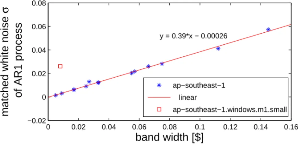
y = 0.39*x − 0.00026 ap−southeast−1 linear ap−southeast−1.windows.m1.smallFig. 4. Standard deviation of the white noise of the matchedAR(1)process as a function of artificial price-band width
price is the price corresponding to the knee in the graph (shown in the same figure), or the maximal price if no knee exists. We refer to this price range, in which availability is a linear function of the price, as the pricingband. The algorithm dynamically changes the reserve price such that there is a linear relation between availability and prices in the floor–ceiling range. It guarantees that the reserve price never drops below the floor, which reflects Amazon’s minimal-reserve price for spot instances, nor rises above the ceiling.
We deconstruct the reserve price algorithm using traces from April–July 2010, when the spot price in eight ap-southeast.windows instance types almost always stayed within the artificial band. We matched the price changes in those traces (denoted by ∆) with an AR(1) (auto-regressive) process. We found a good match (i.e., negligible coefficients of higher ordersaifori >1) to the following process:
∆i=−a1∆i−1+(σ), (1)
where a1 = 0.7 and (σ)is white noise with a standard deviationσ. LetF, C denote
the floor and ceiling of the artificial band, respectively. We matched σ with a value of 0.39(C−F). These parameters fit all the analyzed types well, except form1.small, which matched different values (a1= 0.5, σ= 0.5(C−F)). The standard deviations are
given in Fig. 4. This close fit—the same parameters characterizing the randomness of several different traces—is consistent with our hypothesis that the prices are usually set by an artificial algorithm. The reason form1.small’s deviation is yet to be found.
On the basis of this analysis, we construct theAR(1)reserve price algorithm: The process is initialized with a reserve price ofP0=F and a price change of∆0= 0.1(F−
C). The following prices are defined as Pi = Pi−1 + ∆i, where ∆i = −0.7·∆i−1+
(0.39·(C−F)). The process is truncated to the[F, C]range by regenerating the white noise component whilePiis outside the[F, C]range or identical toPi−1. All prices are
rounded to one-tenth of a cent, as done by Amazon during 2010.
To evaluate whether the trace produced by the truncatedAR(1)process matches the original EC2 trace, we compare their periodograms (normalized Fourier transforms) in Fig. 5. The periodogram comparison verifies that we captured the original signal’s
0 0.1 0.2 0.3 0.4 0.5 0.6 0.7 0.8 0.9 1 −100 −90 −80 −70 −60 −50 −40
Normalized frequency (
×
π
rad/sample)
One−sided PSD
(dB/rad/sample)
PSD estimatate of EC2 ap−southeast tracePSD estimatate of AR(1) process
Fig. 5. Power spectral density (periodogram) estimate of an EC2 price trace, and our derivedAR(1)price trace
frequencies correctly, and not just the average time in each price. The match shows that our reverse-engineered reserve price algorithm is consistent with Amazon’s.
The consistency of anAR(1)process with the EC2 traces does not indicate the dy-namics which create it. If this consistency can be explained mostly by natural fluctu-ations, then we would expect to see at least a weekly cycle. A daily cycle is unlikely, since clients all over the world use the same machines.
To search for a weekly cycle, we analyzed the utilization of memory in three IaaS pay-as-you-go cloud traces (described in detail in Section 6.2) and the price in the ap-southeast.linuxtraces. We computed each day’s mean value (price or utilization for spot trace or cloud, respectively), taking into consideration the duration for which the value was valid. Each day’s mean value was normalized by the mean value over the week to which it belongs. This local normalization is especially important when computing mean utilization, since over the years of the trace, both the capacity and the utiliza-tion increased. The autocorrelautiliza-tion of cloud utilizautiliza-tion for three cloud workloads is depicted in Fig. 6a. All three clouds have a significant weekly cycle, sometimes with a pattern lasting for several weeks. The weekly cycle is expressed by strong, positive autocorrelation coefficients for lags of 7, 14, 21 and even 28 days. In addition, there is strong positive autocorrelation with the previous day, meaning today’s utilization is a good prediction for tomorrow. The confidence bounds are low (0.081, 0.084, 0.068) and slightly different from one.
Knowing autocorrelation can be expected in a cloud, let us turn to analyze the spot price autocorrelation that is depicted in Fig. 6b. The confidence bounds are larger than in the cloud load graphs, and are identical to the fifth digit (0.2097). None of the eight price traces has any weekly cycle or any significant long range correlation. This finding agrees with Wee [2011], who shows that none of the 64 EC2 traces we used exhibit notable weekly or daily patterns. Moreover, the one-day autocorrelation coefficients are negative for all the traces, meaning today’s price is a bad prediction for tomorrow. Thus, the process generating the traces cannot be explained mostly by natural fluctuations.
Let us consider the hypothesis that natural dynamics account for a small part of the trace: usually the spot price is the dynamic reserve price, but sometimes the spot price rises above the reserve price due to market considerations. This would mean that usually the price traces reflect the reserve price only, but sometimes the prices are
0 5 10 15 20 25 30 −0.4 −0.2 0 0.2 0.4 0.6 0.8 1 Lag (days) Sample autocorrelation function of normalized daily mean load
cloud 1 cloud 2 cloud 3
(a) Memory utilization of three clouds
0 5 10 15 20 25 30 −0.4 −0.2 0 0.2 0.4 0.6 0.8 1 Lag (days)
Sample autocorrelation function of normalized daily mean price
m1.small m1.large m1.xlarge m2.xlarge m2.2xlarge m2.4xlarge c1.medium c1.xlarge
(b) Price of eightap-southeast.linuxtypes Fig. 6. Autocorrelation of mean daily values (memory utilization or prices), with respective approximate confidence bounds are displayed as horizontal lines in the same colors as the autocorrelation curves. The daily values are normalized by their week’s mean value.
Dec Jan Feb Mar Apr May Jun Jul
0.4 0.5 0.6 0.7 0.8 0.9 1
date (Dec 2009 − Jul 2010)
normalized spot price
2nd epoch 1st epoch 3rd epoch low prices tran− si− tion
low and high prices highprices new
min. price
Fig. 7. Price history forus-east.windows.m1.small. Three time epochs are shown, with a transition period between the second and third epochs. The spot price is presented as a fraction of the on-demand price for the same instance.
bids declared by real clients. This scenario is unlikely because, as discussed earlier, bidding inside the band is not cost-effective. Nonetheless, we check this hypothesis by analyzing mean trace prices, with the alternate hypothesis that natural dynamics account for no part of the trace. If the alternate hypothesis is true, the mean trace price should be the mean of the truncatedAR(1)process, which is a symmetric process: the middle of the band. If natural dynamics sometimes raise the price above the reserve price, the mean price should be higher than the middle of the band. However, for the 8 ap-southeast.windowstraces we tested here, the mean price waslowerthan the middle of the band by up to 2%.
We conclude that the impact of natural dynamics on the price traces in the band range is statistically insignificant. The spot price within the band is almost always determined solely by the AR(1) process, i.e., is equal to the reserve price. Since we assume prices above the band usually result from natural dynamics, we need to es-timate how frequently the prices are above the band. On average, over the 64 traces we analyzed, prices were above the band 2% of the time. We conclude that during the other 98% of the time, prices are mainly determined by an artificial AR(1) reserve price algorithm and hardly ever represent real client bids.
5. PRICING EPOCHS
To statistically analyze spot price histories, it would be erroneous to assume that the same pricing model applies to all the data in the history trace. Rather, each trace is divided to contiguous epochs associated with different pricing policies. We show here that our main traces are divided into three epochs as depicted in Fig. 7. Since the pricing mechanism changes notably and qualitatively between epochs, data regarding these epochs should be separated if an associated statistical analysis is to be sound. Accordingly, for the purpose of evaluating the effectiveness of client algorithms, strate-gies, and predictions, the data from a (single) epoch of interest should be used.
Thefirst epochstarts, according to our analysis, as early as 30 November 2009 and ends on 14 December 2009, the date on which Amazon announced the availability of spot instances. During this time, instances were unknown to the general public. Hence, the population which undertook any bidding during the first epoch was smaller than the general public, of nearly constant size, and possibly had additional information regarding the internals of the pricing mechanism at that time.
The second epoch begins with the public announcement on 14 December 2009. It ends with a pricing mechanism change around 8 January 2010, when minimal spot prices abruptly change in most instances (usually decrease, though Fig. 7 demon-strates an increase). It is characterized by long intervals of constant low prices.
The third epoch begins on 20 January 2010. Instance types and regions began to change minimal price around January 8th, but we define the beginning of the epoch as the date in which the last one (eu-west.linux.m2.2xlarge) reached a new minimal price. Due to (1) the gradual move to the new minimal values and to (2) a bug in the pricing mechanism that was fixed in mid-January 2010 [Amazon 2010], we choose to disregard data from the transition period between the second and third epochs.
Additional epoch-defining dates are dates when the price-change timing algorithm was changed, e.g., 20 July 2010 and 9 February 2011 for theus-eastregion (see Sec-tion 6).
These abrupt time-correlated changes in many regions and instance types further support our hypothesis, since prices are likely to undergo abrupt changes at exactly the same time either when the market is efficient (which is not the case here, since absolute prices in Fig. 1 are not leveled) or when the prices are artificial.
6. SPOT PRICE SIMULATION
To get a better feel for the validity of our hypothesis, we simulated two spot pricing systems, representing the dynamic hidden reserve price hypothesis and the alternate hypothesis of a constant reserve price. Both systems are based on a sealed-bid(N+1)th
price auction with a reserve price with retroactive supply limitation, as described in Section 4.1. The simulator structure is described in Section 6.1.
In both systems we set the on-demand price to 1. In the constant reserve price sys-tem we set the reserve price to 0.4. In the AR(1) reserve price syssys-tem we set the reserve prices according to the reserve price algorithm defined in Section 4.3, with a band of [0.4,0.45]. To run the simulation, we need to know not only what the new reserve price should be, but also when it should be changed. To this end, we deconstructed the price change timing, as explained in Section 6.4.
To fully model a spot pricing system, three input data sets or models are required: for available machine supply, for instance demand, and for client bids. We modeled the machine supply as a fixed-size, because spot instances are a good practice for a quick-launch buffer: those machines which need to be kept running, in case an on-demand or reserved instance is requested. We do not expect spot-instance machine supply to represent the full variation of on-demand and reserved instance demand. We used real
(Section 6.3). The simulation results are presented in Section 6.5.
6.1. Simulator Event-Driven Loop
We created a trace-based event-driven simulator, where events are: (1) instance sub-mission and termination and (2) price changes (due to a scheduled change or to a waiting instance with a bid higher than the spot price). We ran the grid trace-driven simulation on 70 CPUs, according to the number of CPUS in the trace. Since CPU was over-committed on the cloud traces but physical memory was not, we defined each cloud’s capacity as the maximal amount of memory concurrently used in its trace. We ended the simulation when the last input-trace job had been submitted.
6.2. Workload Modeling
We fed the simulation with tasks with run-times in the range of 10 minutes to 24 hours, taken from several large system traces. According to Iosup et al. [2011], a typical EC2 instance overhead is two minutes. We deem clients unlikely to wait two minutes and pay for a full hour for an activity which lasts only a few minutes, so we only used tasks longer than 10 minutes. We assume spot instances are usually used for relatively short-running instances, with longer running instances more likely to be deployed on more stable offerings such as on-demand and reserved instances. Thus we omitted tasks longer than 24 hours. We discuss the task length cut-off point in Section 6.5.
We used traces from one grid and three clouds. In the simulation, each task was interpreted as a single instance, submitted at the same time and requiring the same run-time as in the original trace to complete. The grid trace is 20K tasks from the LPC-EGEE workload1. LPC-EGEE is characterized by tasks which are small in comparison to the capacity of the cluster, allowing for elasticity.
We also used traces of three pay-as-you-go IaaS clouds2. These clouds were partitions of IBM’s RC2 cloud [Ryu et al. 2011]. The partitions used different underlying physical resources and hypervisors, and it was up to the user to choose the partition. The traces were taken from 2 April 2009 to 22 August 2011 (2.5 years). During this time, the capacity of the partitions changed with demand, reaching concurrent use of thousands of CPUs (6522, 1420, and 845 for clouds 1, 2, and 3, respectively) and thousands of gigabytes of memory (10175, 1996, and 2386 for the respective clouds). Clients of these clouds were charged 2-3 cents per hour per GB for running instances. In addition, creating an instance for the first time cost 20 cents.
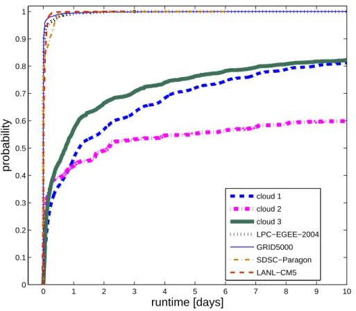
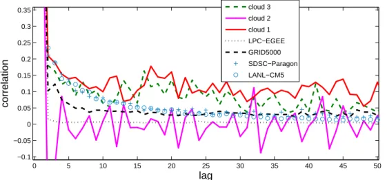
The workloads of these clouds are characterized by significantly longer runtimes than grid jobs: only half the cloud instances take less than 24 hours, while 98% of the tasks last less than a day on grids (LPC-EGEE, GRID50003) and parallel sys-tems (LANL CM-54, SDSC-Paragon5) that we evaluated, as seen in Fig. 8. Many cloud instances last months and even years. Furthermore, the clouds exhibit longer and stronger inter-arrival time correlation than typical grids, as seen in Fig. 9. The au-tocorrelations of their inter-arrival times is even larger than those of parallel systems, even though both system types are only accessible to a limited set of clients.
1Graciously provided by Emanuel Medernach [2005], via the Parallel workload archive [Feitelson ], file LPC-EGEE-2004-1.2-cln.swf.
2Graciously provided by Mariusz Sabath.
3Graciously provided by Franck Cappello, via the Grid Workloads Archive [Iosup et al. 2008], file grid5000 clean trace.swf.
4Graciously provided by Curt Canada, via the Parallel workload archive, file LANL-CM5-1994-3.1-cln.swf. 5Graciously provided by Reagan Moore and Allen Downey, via the Parallel workload archive, file SDSC-Par-1995-2.1-cln.swf.
0 1 2 3 4 5 6 7 8 9 10 0 0.1 0.2 0.3 0.4 0.5 0.6 0.7 0.8 0.9 1
runtime [days]
probability
cloud 1 cloud 2 cloud 3 LPC−EGEE−2004 GRID5000 SDSC−Paragon LANL−CM5Fig. 8. CDF of instance or task runtimes on clouds, parallel systems and grids 6.3. Customer Bid Modeling
Due to the lack of information on the distribution of real client bids (since we argue that Amazon’s price traces supply little information of this type), we compare several bidding models, and verify that the qualitative results are insensitive to the bid mod-eling. All the distributions were adjusted to uniform minimal and on-demand prices.
The first model is a Pareto distribution (a widely applicable economic distribu-tion [Souma 2002; Levy and Solomon 1997]) with a minimal value of 0.4, and a Pareto index of 2, a reasonable value for income distribution [Souma 2002]. The second model is the normal distribution N(0.7,0.32), truncated at 0.4. The third is a linear map-ping from runtimes to (0.4,1], which reflects client aversion to having long-running instances terminated.
6.4. Price Change Timing
Price changes in the simulation are triggered according to the cumulative distribution function (CDF) of intervals between them, collected during January–July 2010, and given in Fig. 10 (solid line). This period was characterized by quiet times—prices never changed before 60 minutes or between 90 and 120 minutes since the previous price change. It is interesting to note that such quiet times can be monetized by clients to gain free computation power with a probability of about 25%, by submitting an
0 5 10 15 20 25 30 35 40 45 50 −0.1 −0.05 0 0.05 0.1 0.15 0.2 0.25 0.3 0.35 lag correlation cloud 3 cloud 2 cloud 1 LPC−EGEE GRID5000 SDSC−Paragon LANL−CM5
Fig. 9. Task/instance inter-arrival time autocorrelation on clouds, parallel systems (LANL CM-5, SDSC), and grids (LPC-EGEE, GRID5000).
0 1 2 3 4 5 6 7 8 9 0 0.2 0.4 0.6 0.8 1
step length: time between price changes [h]
probability
Jan 2010 − Jul 2010Jul 2010 − Feb 2011
Feb 2011 − April 2011 (present day)
Fig. 10. CDF of time interval between price changes for different versions of the price change scheduling algorithm. Input:us-east.linux.m1.small.
instance with a bid of the current spot price 31 minutes after a price change. The instance would then have a 50% possibility of undergoing another price change within 30-60 minutes. If that change is a price increase, the instance would be terminated, and the client would gain, on average, 45 minutes of free computation. Clients do not exploit this loophole in our simulation.
Fig. 10 also presents the evolution of the timing of price changes for the us-east region. The next algorithm (in place from July 2010 until 8 Feb 2011) allowed for a quiet hour after a price change. The following one (starting 9 Feb 2011) matches an exponential distribution with a 1.5 hour rate parameter, with five quiet minutes. This almost memory-less algorithm prevents abuse of the timing algorithm. A similar
evolution of the algorithm took place in other regions on different dates. On Linux instances in regions other than us-east, an interim algorithm was used between the second and third algorithms, such that the quiet hour was abolished before the transfer to the algorithm of 2011. 6.5. Simulation Results 0.4 0.45 0.5 0.55 0.6 0.65 0.7 0.75 0.8 0.85 0.9 0 0.1 0.2 0.3 0.4 0.5 0.6 0.7 0.8 0.9 1
declared price as fraction of on−demand price
availability fraction Const. reserve price, Pareto dist.AR(1) band of reserve price, Pareto dist.
Const. reserve price, Linear by task length dist. AR(1) reserve price, Linear by task length dist. Const. reserve price, Normal dist. AR(1) band of reserve price, Normal dist.
(a) LPC-EGEE 0.4 0.45 0.5 0.55 0.6 0.65 0.7 0.75 0.8 0.85 0.9 0 0.1 0.2 0.3 0.4 0.5 0.6 0.7 0.8 0.9 1
declared price as fraction of on−demand price
availability fraction
Const. reserve price, Pareto dist. AR(1) band of reserve price, Pareto dist. Const. reserve price, Linear by task length dist. AR(1) band of reserve price, Linear by task length dist. Const. reserve price, Normal dist.
AR(1) band of reserve price, Normal dist.
(b) Cloud 1 0.4 0.45 0.5 0.55 0.6 0.65 0.7 0.75 0.8 0.85 0.9 0 0.1 0.2 0.3 0.4 0.5 0.6 0.7 0.8 0.9 1
declared price as fraction of on−demand price
availability fraction
Const. reserve price, Pareto dist. AR(1) band of reserve price, Pareto dist. Const. reserve price, Linear by task length dist. AR(1) band of reserve price, Linear by task length dist. Const. reserve price, Normal dist.
AR(1) band of reserve price, Normal dist.
(c) Cloud 2 0.4 0.45 0.5 0.55 0.6 0.65 0.7 0.75 0.8 0.85 0.9 0 0.1 0.2 0.3 0.4 0.5 0.6 0.7 0.8 0.9 1
declared price as fraction of on−demand price
availability fraction
Const. reserve price, Pareto dist. AR(1) reserve price, Pareto dist. Const. reserve price, Linear by task length dist. AR(1) reserve price, Linear by task length dist. Const. reserve price, Normal dist. AR(1) reserve price, Normal dist.
(d) Cloud 3
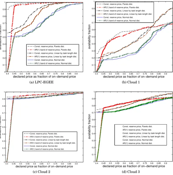
Fig. 11. Simulation results for various bidding models, with constant andAR(1)reserve price, on the basis of a grid trace (LPC-EGEE) and three cloud traces
Simulation results in terms of price-availability graphs are presented in Fig. 11, for different input traces, bid models and price setting mechanisms. The functions of simu-lations with theAR(1)reserve price feature a linear segment and a knee in high avail-ability, as do the availability functions of EC2 during the third epoch, which are shown
0.41 0.42 0.43 0.44 0.45 0.46 0.47 0.48 0.49 0.5 0.51 0.65 0.7 0.75 0.8 0.85 0.9 0.95
declared price as fraction of on−demand price
availability fraction
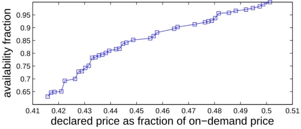
Fig. 12. Availability as a function of the declared price during the second epoch forus-west.linux.m1.xlarge. in Figs. 1, 2, and 3. The constant reserve price functions do not exhibit this behav-ior. Rather, they are jittery, like the high price regime of theus-east.windows.m1.small graph in Fig. 3, and the second epoch graph in Fig. 12. These results are not sensitive to our of choices of bidding model and workload.
Furthermore, the availability of the reserve price in the constant reserve price sim-ulations is high (0.2-0.9), as it is in the second epoch (0.63 in Fig. 12). In contrast, the availability of the minimal price in theAR(1)reserve price simulations and in the third epoch tends to zero as the number of discrete prices within the band grows.
These macro-economic qualitative differences can be better understood by focusing on three classes of availability graphs that resemble one another and do not present straight lines: (1) the constant minimal reserve price simulations, (2) the second epoch, and (3) the high regime of the third epoch (in particular us-east.windows.m1.small). Since the graphs of the first class reflect client bids, the qualitative resemblance sug-gests that the last two also reflect client bids: during the second epoch, a constant reserve price algorithm is used, and the demand forus-east.windows.m1.smallexceeds the supply so much that excess demand is no longer masked by the dynamic reserve price.
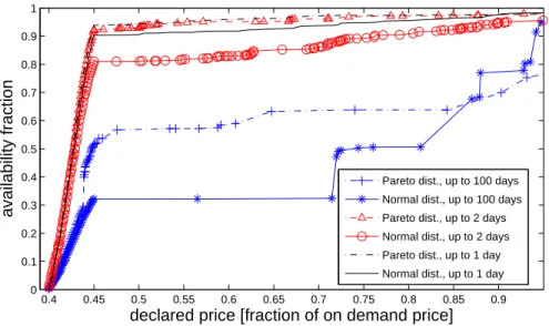
To investigate the effect of truncating long running instances from the traces (mainly from the cloud traces), we ran the AR(1) simulations with different maximal run-time truncations (1 day, 2 days and 100 days). As can be seen from the price-availability graphs (Fig. 13), raising the upper truncation point of the trace lowers the availability at the knee. The truncation does not affect the important features discussed earlier (the straight line and the existence of the knee). From the EC2 traces we learn that the knee is usually high (above 0.9, with the exception of somem1.small instances). Thus we conclude that the workload of Amazon’s EC2 spot instances is consistent with relatively short instances, and that our choice of truncating the traces at 24 hours is reasonable.
We consider these simulation results a constructive indication that most prices in the EC2 traces during the third epoch are set using anAR(1)reserve price, which is not market driven. The simulation results also suggest that Amazon set prices via a market-driven auction with a constant reserve price during the second epoch (Decem-ber, 2009 until January, 2010), and that prices above the band are market-driven. (In the traces we studied, prices are above the band only 2% of the time on average.)
0.4 0.45 0.5 0.55 0.6 0.65 0.7 0.75 0.8 0.85 0.9 0 0.1 0.2 0.3 0.4 0.5 0.6 0.7 0.8 0.9 1
declared price [fraction of on demand price]
availability fraction
Pareto dist., up to 100 days Normal dist., up to 100 days Pareto dist., up to 2 days Normal dist., up to 2 days Pareto dist., up to 1 day Normal dist., up to 1 day
Fig. 13. Impact of running time truncation of the cloud 2 trace on price-availability graphs for simulations with Pareto and normally distributed bids and AR(1) reserve price
7. DYNAMIC RESERVE PRICE BENEFITS
The dynamicAR(1)reserve price mechanism has several long-term, wide-range ben-efits that may justify its use. Like a constant minimal or reserve price, it guarantees that on-demand instances are not completely cannibalized by spot instances. Yet it also allows the provider to sell instances on machines which would otherwise run idle, to provide elasticity for the fixed price instances. Spot instances, which can be quickly evacuated, still reduce the costs associated with idle servers, with no real harm to the main offering of on-demand instances.
Using a hidden reserve price allows the provider to change the reserve price with no obligation to inform the clients, an obligation which cannot be avoided when using a minimal price. A dynamic reserve price is better than a constant minimal price, because it maintains an impression of constant change, thus preventing clients from becoming complacent. It forces them to either bid higher than the band or tolerate sudden unavailability. It also serves to occasionally clear queues of low bids within the band, a purpose that is not served by a constant reserve price that is equal to the ceiling price. Furthermore, Vincent [1995] argues that in common value English and second price auctions, a random reserve price encourages participation, and thus the exchange of more information about the value of the goods.
A random reserve price might also serve other goals, if the public is unaware of its use. By creating an impression of false activity (demand and supply changes), the random reserve price can mask times of low demand and price inactivity, thus possibly driving up the provider’s stock. A large enough band covering the spectrum of probable prices could also mask high demand and low supply, and thus help to maintain the illusion of an infinitely elastic cloud. However, if the artificial band is relatively small, as in the case of Amazon EC2 spot prices, the provider’s use of anAR(1)process for setting the price within the band is a strong indication of low demand.
We will now review the literature on pay-as-you-go IaaS cloud workload traces (and spot prices in particular), reexamining past conclusions in light of our results. We will also review literature on computation markets and on reserve prices, examining the implications of these works on our results.
Cloud Traces. IaaS pay-as-you-go cloud workload traces and models are so hard to come by that researchers like Toosi et al. [2011] resorted to a grid and parallel systems model [Lublin and Feitelson 2003] with adapted runtime parameters to describe cloud workloads. Google [Hellerstein et al. 2011] released two backend workload traces, the longest of which lasts 29 days. Liu [2011] measured week-long traces of CPU utiliza-tion of EC2 machines, showing a strong daily pattern of the guest machines on the measured host. This pattern indicates that clients prefer to keep instances running idle rather than shut them off for the night. Such client behavior weakens the daily cycle of demand for EC2 machines in general (not necessarily spot instances).
Reserve Prices. Li and Tan [2000] showed that a (hidden) reserve price improves rev-enues of first price, sealed bid auctions for risk-averse clients. Li and Perrigne [2003] showed that for first price sealed bid auctions, an optimal announced minimal price in-creases the seller’s revenue compared with an arbitrary reserve price. They used data of timber sales in Canada. Katkar and Reiley [2006] found that for low-priced eBay sales of up to $20, (hidden) reserve prices deter good clients and yield lower revenues than minimal (published) prices. However, none of these works relate to anN+1th
auc-tion with arandom reserve price. Ramberg [2002] says that “the existence of a hidden reserve price is to a great extent similar to the situation where the invitor is bidding.” She recommends that when the auction is run by the invitor (as is the case with Ama-zon’s spot instances), “. . . it should not be a second price auction, or otherwise there should be some assurance that the invitor/operator will not submit bids.”
Analyzing Spot Price Traces.Concurrently with this work, Wee [2011] also analyzed price-availability graphs of early EC2 traces, noted the knees and the different be-havior of m1.small, and that the average price does not change over time. Wee only analyzed epochs in which the timing of price changes always included a quiet hour and assumed that Amazon does not have an incentive to change prices more often than once an hour. However, as we show in Section 6.4, Amazon’s early price change timing was a vulnerability, incentivizing it to change prices more frequently than once an hour, as it later did. Wee [2011] and Javadi and Buyya [2011] also checked EC2 price traces for cycles. Javadi and Buyya, who computed various price trace statis-tics, claimed spot prices have daily and weekly cycles, but Wee found that cycles are statistically insignificant. Our findings for theap-southeastregion agree with Wee’s.
Using Spot Price Traces for Client Strategy Evaluation.Most studies that use price traces use them to evaluate client strategies. The relevance of such work to future de-ployment of instances needs to be re-evaluated when the nature of the traces changes (i.e., when a new epoch starts). Andrzejak, Kondo and Yi used spot price histories to advise the client how to minimize monetary costs while meeting an SLA [Andrzejak et al. 2010], and to schedule checkpoints [Yi et al. 2010] and migrations [Yi et al. 2011]. The first two works used data from the transition period between the second and third epoch for their evaluation. They focused on eu-west, which suffered most from this transition. The last interchangeably used data from before and after the change in the price change algorithm on July 25, 2010, as did Voorsluys et al. [2011].
Mattess et al. [2010] examined client strategies for using spot instances to manage peak loads on scientific workloads. They evaluated the strategies using an EC2 spot
instance trace of the third epoch only, attributing the different trace behavior prior to January 18th, 2010 to Christmas and to the recent introduction of spot instances. They identified the price band, noted that bidding just above the band is almost as good as bidding very high, and recommended bidding right under the on-demand price.
Chohan et al. [2010] processed price histories to answer the question, What is the probability that an instance with a certain bid price would last a certain time? They analyzed price histories from the third epoch only, because of the pricing bug that was fixed in mid-January 2010 [Amazon 2010]. The bug allowed instances with prices higher than the regional spot price to be terminated due to congestion in their avail-ability zone (which is a part of the region), while keeping the regional price low. The authors attributed the qualitative change of prices between the second and third epoch to the bug fix. However, this bug fix is unlikely to have caused the qualitative price changes we observe during January 2010, namely, the appearance of the pricing band. The authors also noted the cost-effectiveness of bidding at the top of the band.
Wieder et al. [2010] described a model for optimizing map-reduce on clouds using a utility function that depends on execution time, data transfer costs, and computation costs, which they assumed can be predicted for spot instances.
Brebner and Liu [2011] assessed cost and performance of various clouds, including spot instances. They represented the cost of spot instances as a constant, which equals the average of several months of the price trace, but did not state the duration or length of the history they used. It is thus impossible to determine which epochs they used, and what the given average values represent.
Vermeersch [2011] analyzed spot price histories with the goal of optimizing the client’s choice of deals on EC2.
Zhao et al. [2012] and Mazzucco and Dumas [2011] assumed spot instance prices are market-driven, and modeled some of them to be used as a client decision aid. These models are no longer relevant once a drastic policy change is made.
Using Spot Price Traces to Learn about the Market.Zhang et al. [2011] assumed Amazon uses a market-driven auction, which led them to conclude that spot price histories reflect actual client bids. On this basis they sought resource allocations to instance types which optimized the provider’s revenue. Chen et al. [2011], who tested provider scheduling algorithms, likewise assumed EC2 price traces represent market clearing prices. We consider these assumptions doubtful, in light of our findings that 98% of the time, on average, EC2 price traces are the reserve prices, and as such do not provide a lot of information about real client bids, nor are necessarily clearing prices.
Free Spot and Futures Markets. While Amazon is currently the only provider offering “spot instances,” free computing resource markets have already been analyzed. Ortuno and Harder [2010] modeled a free market for computing power. Altmann et al. [2008] described GridEcon, a foundation for a free spot and futures market. Vanmechelen et al. [2011] modeled a free market for computing power using spot and futures deals. Price traces of such free markets [Ortuno and Harder 2010; Vanmechelen et al. 2011] differ from EC2 spot price traces: they do not have a hard minimal price and are not anchored in the bottom of the price range. Rahman et al. [2011] evaluated free spot market options using EC2 traces, and noted that the “data does not show enough fluc-tuations as expected in a free market.”
9. CONCLUSIONS
Amazon EC2 spot price traces provide more information about Amazon than about its clients. We have shown that during the examined period Amazon probably set spot prices using a random AR(1) (hidden) reserve price. This price might have been the basis of a market-driven mechanism, in which high prices might have reflected market
the dynamic reserve price.
Understanding how Amazon prices its spare capacity is useful for clients, who can decide how much to bid for instances; for providers, who can learn how to build more profitable systems; and for researchers, who can differentiate between prices set by an artificial process and prices likely to have been set by real client bids. We have shown that many price trace characteristics (e.g., minimal value, band width, change timing) are artificial and might change according to Amazon’s decisions. Thus, researchers should be aware of the epochs present in their traces when using those traces to model future price behavior or to evaluate client algorithm performance. We have shown that indiscriminately using Amazon’s current traces to model client behavior is unfounded on average 98% of the time for the examined period.
10. EPILOGUE
Amazon’s EC2 spot instance pricing mechanism underwent a radical change between the first submission of this paper and its first acceptance. Several days after its ac-ceptance, the spot instance prices underwent another extreme change, and the pric-ing band disappeared from the traces altogether. For example, in the trace shown in Fig. 14, the spot price is constant throughout October 2011, except for a change in the minimal price. While these radical qualitative changes are further evidence of the former prices being artificially set, the October prices are consistent with a constant minimal price auction, and are no longer consistent with an AR(1) hidden reserve price. 0 1 2 3 4 5 6 7 8 9 0.5 0.6 0.7 0.8 0.9 1 1.1 Time (Months of 2011)
Spot instance price (normalized)
us−east−1.suse.m1.large
Paper accepted First paper
submitted End of data
used for the paper
Paper rejected, Tech report published, Tweeted and re−Tweeted
to thaousands of people
Fig. 14. The history of this paper and the price trace ofsuse.m1.largeonus-eastduring 2011
ACKNOWLEDGMENTS
We gratefully acknowledge the generous assistance and valuable information provided to us by Mariusz Sabath and Yaron Wolfsthal of IBM Research.
REFERENCES
AGMONBEN-YEHUDA, O., BEN-YEHUDA, M., SCHUSTER, A.,ANDTSAFRIR, D. 2011. Deconstructing
Ama-zon EC2 spot instance pricing. InIEEE Third International Conference on Cloud Computing Technology and Science (CloudCom).
ALTMANN, J., COURCOUBETIS, C., STAMOULIS, G., DRAMITINOS, M., RAYNA, T., RISCH, M.,ANDBAN
-NINK, C. 2008. GridEcon: A market place for computing resources. InGrid Economics and Business Models. Lecture Notes in Computer Science Series, vol. 5206. Springer Berlin / Heidelberg, 185–196. Amazon 2009. Amazon EC2 spot instances.http://aws.amazon.com/ec2/spot-instances/. [Accessed Aug.
2011].
Amazon 2010. Spot instance termination conditions?http://tinyurl.com/2dzp734. Online AWS Developer Forums discussion. [Accessed Apr. 2011].
ANDRZEJAK, A., KONDO, D.,ANDYI, S. 2010. Decision model for cloud computing under SLA constraints. In
IEEE/ACM International Symposium on Modelling, Analysis and Simulation of Computer and Telecom-munication Systems (MASCOTS).
BREBNER, P.AND LIU, A. 2011. Performance and cost assessment of cloud services. InService-Oriented
Computing. Lecture Notes in Computer Science Series, vol. 6568. 39–50.
CHEN, J., WANG, C., ZHOU, B. B., SUN, L., LEE, Y. C.,ANDZOMAYA, A. Y. 2011. Tradeoffs between profit and customer satisfaction for service provisioning in the cloud. InHPDC.
CHOHAN, N., CASTILLO, C., SPREITZER, M., STEINDER, M., TANTAWI, A.,ANDKRINTZ, C. 2010. See spot
run: using spot instances for mapreduce workflows. InUSENIX Conference on Hot Topics in Cloud Computing (HotCloud).
FEITELSON, D. Parallel workloads archive. Website. http://www.cs.huji.ac.il/labs/parallel/
workload/index.html.
HELLERSTEIN, J. L., CIRNE, W.,ANDWILKES, J. 2011. Google cluster data. Website.http://code.google.
com/p/googleclusterdata/.
IOSUP, A., LI, H., JAN, M., ANOEP, S., DUMITRESCU, C., WOLTERS, L.,ANDEPEMA, D. H. J. 2008. The Grid Workloads Archive.Future Generation Comp. Syst. 24,7, 672–686.
IOSUP, A., OSTERMANN, S., YIGITBASI, N., PRODAN, R., FAHRINGER, T., ANDEPEMA, D. 2011. Perfor-mance analysis of cloud computing services for many-tasks scientific computing.IEEE Trans. on Paral-lel and Distrib. Sys. (ITPDS) 22,6, 931–945.
JAVADI, B. AND BUYYA, R. 2011. Comprehensive statistical analysis and modeling of spot instances in
public cloud environments. Tech. Rep. CLOUDS-TR-2011-1, Cloud Computing and Distributed Systems Laboratory, The University of Melbourne.
KATKAR, R.ANDREILEY, D. H. 2006. Public versus secret reserve prices in ebay auctions: Results from a
pok´emon field experiment.The B.E. Journal of Advances in Economic Analysis and Policy 5,2.http: //www.degruyter.com/view/j/bejeap.2006.5.2/bejeap.2006.6.2.1442/bejeap.2006.6.2.1442.xml.
LEVY, M.ANDSOLOMON, S. 1997. New evidence for the power-law distribution of wealth.Physica A 242,
90–94.
LI, H.ANDTAN, G. 2000. Hidden reserve prices with risk-averse bidders. Tech. rep., University of British Columbia.
LI, T.ANDPERRIGNE, I. 2003. Timber sale auctions with random reserve prices.Review of Economics and
Statistics 85,1, 189–200.
LIU, H. 2011. A measurement study of server utilization in public clouds. InInt’l Conference on Cloud and Green Computing (CGC).
LOSSEN, T. 2010. Cloud exchange.http://cloudexchange.org/. [Accessed Apr. 2011. The dataset is
avail-able fromhttp://files.evercu.be/cloudexchange.tgz].
LUBLIN, U.ANDFEITELSON, D. G. 2003. The workload on parallel supercomputers: modeling the
charac-teristics of rigid jobs.J. Parallel Distrib. Comput. 63, 1105–1122.
MATTESS, M., VECCHIOLA, C.,ANDBUYYA, R. 2010. Managing peak loads by leasing cloud infrastructure
services from a spot market. InIEEE Int’l Conference on High Performance Computing and Communi-cations (HPCC).
MAZZUCCO, M.AND DUMAS, M. 2011. Achieving performance and availability guarantees with spot
in-stances. InIEEE Int’l Conference on High Performance Computing and Communications (HPCC).
MEDERNACH, E. 2005. Workload analysis of a cluster in a grid environment. InWorkshop on Job Scheduling
Strategies for Parallel Processing.
ORTUNO, F. M.ANDHARDER, U. 2010. Stochastic calculus model for the spot price of computing power. In
Annual UK Performance Engineering Workshop (UKPEW).
RAHMAN, M. R., LU, Y.,ANDGUPTA, I. 2011. Risk aware resource allocation for clouds. Tech. rep.,
Univer-sity of Illinois at Urbana-Champaign.
KARVE, A., LEE, H., LINDEMAN, J. A., MOHINDRA, A., OESTERLIN, B., PACIFICI, G., PENDARAKIS, D., REIMER, D.,ANDSABATH, M. 2011. RC2—living lab for cloud computing. InUSENIX Large Instal-lation Systems Administration Conference (LISA).
SAMOVSKIY, D. 2011. Amazon EC2 spot instances - a flop?http://tinyurl.com/somic11. [Accessed Sep.
2011].
SOUMA, W. 2002. Physics of personal income.http://arxiv.org/pdf/cond-mat/0202388.
TOOSI, A. N., CALHEIROS, R. N., THULASIRAM, R. K.,ANDBUYYA, R. 2011. Resource provisioning policies to increase iaas provider s profit in a federated cloud environment. InIEEE Int’l Conference on High Performance Computing and Communications (HPCC).
VANMECHELEN, K., DEPOORTER, W.,ANDBROECKHOVE, J. 2011. Combining futures and spot markets: A
hybrid market approach to economic grid resource management.Journal of Grid Computing 9, 81–94.
VERMEERSCH, K. 2010. Spot watch.http://spotwatch.eu/input/. [Accessed Apr. 2011. The dataset and
website code are available fromhttps://s3-eu-west-1.amazonaws.com/ruben.ruben/SpotWatch.tar].
VERMEERSCH, K. 2011. A broker for cost-efficient QoS aware resource allocation in EC2. M.S. thesis,
Uni-versiteit Antwerpen.
VINCENT, D. R. 1995. Bidding off the wall: Why reserve prices may be kept secret.Journal of Economic
Theory 65,2, 575–584.
VOORSLUYS, W., GARG, S. K.,AND BUYYA, R. 2011. Provisioning spot market cloud resources to create
cost-effective virtual clusters. InICA3PP.
WEE, S. 2011. Debunking real-time pricing in cloud computing. InIEEE/ACM Int’l Symposium on Cluster, Cloud and Grid Computing (CCGrid).
WIEDER, A., BHATOTIA, P., POST, A.,ANDRODRIGUES, R. 2010. Brief announcement: modelling
mapre-duce for optimal execution in the cloud. InACM SIGACT-SIGOPS Symposium on Principles of Dis-tributed Computing (PODC).
YI, S., ANDRZEJAK, A.,ANDKONDO, D. 2011. Monetary cost-aware checkpointing and migration on Ama-zon cloud spot instances.IEEE Transactions on Services Computing.
YI, S., KONDO, D.,AND ANDRZEJAK, A. 2010. Reducing costs of spot instances via checkpointing in the Amazon Elastic Compute Cloud. InIEEE International Conference on Cloud Computing (CLOUD). ZHANG, Q., GURSES, E., BOUTABA, R.,ANDXIAO, J. 2011. Dynamic resource allocation for spot markets
in clouds. InWorkshop on Hot Topics in Management of Internet, Cloud, and Enterprise Networks and Services (Hot-ICE).
ZHAO, H., PAN, M., LIU, X., LI, X.,ANDFANG, Y. 2012. Optimal resource rental planning for elastic appli-cations in cloud market. InIEEE Int’l Parallel & Distributed Processing Symposium (IPDPS).