A Visual Programming Tool for Designing Planning Problems for
Semantic Web Service Composition
Dimitris Vrakas1, Ourania Hatzi2, Nick Bassiliades1, Dimosthenis Anagnostopoulos2 and Ioannis Vlahavas1
1Dept. Of Informatics, Aristotle University Of Thessaloniki, Thessaloniki, 54124, Greece
{dvrakas, nbassili, vlahavas}@csd.auth.gr
2Department of Geography, Harokopio University, Athens, Greece {raniah, dimosthe}@hua.gr
Abstract
This chapter is concerned with the issue of knowledge representation for AI Planning problems, especially those related to Semantic Web Service composition. It discusses current approaches in encoding planning problems using the PDDL formal language and it presents ViTAPlan, a user-friendly visual tool for planning. The tool is built on top of HAPRC, a rule-configurable planning system, which automatically adapts to each problem, in order to achieve best performance. Apart from HAPRC, ViTAPlan can be interfaced with any other planning system that supports the PDDL language. More than just being a user friendly environment for executing the underlying planner, the tool serves as a unified planning environment for encoding a new problem, solving it, visualizing the solution and monitoring its execution on a simulation of the problem’s world. The tool consists of various sub-systems, each one accompanied by a graphical interface, which collaborate with each other and assist the user, either a knowledge engineer, a domain expert, an academic or even an end-user in industry, to carry out complex planning tasks, such as composing complex Semantic Web Services from simple ones, in order to achieve complex tasks. The key feature of ViTAPlan is a visual programming module that enables the user to encode new planning problems just by using visual elements and simple mouse operations. The visual tool performs a validity check on the visual program created by the user
and then compiles it to PDDL files that are ready to be used by any planning system. Finally, the planning system will solve the planning problem and then export the plan in an appropriate Web Service composition language to a Web Service execution monitoring system or just publish it in a UDDI registry.
Keywords: Automated Planning; Graphical Interfaces; Machine Learning; Knowledge Engineering; Semantic Web Service Composition
1. Introduction
Planning is the process of finding a sequence of actions (steps), which if executed by an agent (biological, software or robotic) result in the achievement of a set of predefined goals. The sequence of actions mentioned above is also referred to as plan.
The actions in a plan may be either specifically ordered and their execution should follow the defined sequence (linear plan) or the agent is free to decide the order of executions as long as a set of ordering constraints are met. For example, if someone whishes to travel by plane, there are three main actions that he/she has to take: a) buy a ticket, b) go to the airport and c) board on the plane. A plan for traveling by plane could contain the above actions in a strict sequence as the one defined above (first do action a, then b and finally c), or it could just define that action c (board on plane) should be executed after the first two actions. In the second case the agent would be able to choose which plan to execute, since both a→b→c, and b→a→c sequences would be valid.
The process of planning is extremely useful when the agent acts in a dynamic environment (or world) which is continuously altered in an unpredictable way. For
instance, the auto pilot of a plane should be capable of planning the trajectory that leads the plane to the desired location, but also be able to alter it in case of an unexpected event, like an intense storm.
The software systems that automatically (or semi- automatically) produce plans are referred to as Planners or Planning Systems. The task of drawing a plan is extremely complex and it requires sophisticated reasoning capabilities which should be simulated by the software system. Therefore, Planning Systems make extensive use of Artificial Intelligence techniques and there is a dedicated area of AI called Automated Planning.
Automated Planning has been an active research topic for almost 40 years and during this period a great number of papers describing new methods, techniques and systems have been presented that mainly focus on ways to improve the efficiency of planning systems. However, there are not many successful examples of planning systems adapting to industrial use. From a technical point of view, this can be mainly explained by four reasons: a) There is a general disbelief by managers and workers in industry that AI tools can really assist them, b) There is a need for systems that combine methods from many areas of AI, such as Planning, Scheduling and Optimization, c) The industry needs more sophisticated algorithms than can scale up to solve real-world problems and d) In order for workers in industry to make use of these intelligent systems, they must be equipped with user friendly interfaces that: i) allow the user to intervene in certain points and ii) can reason about the provided solution.
The greatest problems that one faces when he/she tries to contact companies and organizations for installing a planning system, come from the workers themselves. These problems concern two issues: a) It has been noticed that people find it hard to
trust automated systems when it comes to crucial processes. Many people still think that they can do better than machines. b) There is a quite widespread phobia towards computers and automated machines due to the lack of information. A large number of people are afraid of being replaced or governed by machines and they try to defend their posts by rejecting everything new.
Although it is necessary for researchers to specialize in very specific parts of their research area, commercial systems, dealing with real time problems, have to combine techniques and methods from many areas. It has been shown that AI Planning techniques for example, are inadequate to face with the complexity and the generality of real world problems. For example, it has been proven that Scheduling and Constraint solving techniques can handle resources more efficiently. Commercial applications must combine methods from many areas of AI and probably from other areas of computer science as well.
Another issue that must be dealt with is the large gap between toy problems used by researchers for developing and testing their algorithms and the actual problems faced by people in industry. Researchers are usually unaware of the size of real world problems or they simplify these problems in order to cope with them. However, these algorithms prove themselves inadequate to be adopted by commercial software. So it is a general conclusion that researchers should start dealing with more realistic problems. This research direction was also given during the last AIPS Planning competitions where there was a tendency to test planners on problems closer to reality.
Last but certainly not least is the direct need of software based on AI tools to be accompanied with user friendly interfaces. Since the user will be a manager or even a simple worker in a company and not a computer scientist, the software must be easy
to use. Furthermore, it must enable the user to intervene in certain points for two reasons: a) Mixed initiative systems can deal with real-world problems better and b) people in companies do not like to take commands and therefore a black box which can not reason about its output will not do. So it is necessary for the software to cooperate with the user in the process of solving the problem in hand, since people have a more abstract model of the problem in their mind and are better in improvising, while computers can deal with lower levels of the problem more efficiently.
1.1. Semantic Web Service Composition
The Web is becoming more than just a collection of documents; applications and services are coming to the forefront. Web services will play a crucial role in this transformation as they will become the basic components of Web-based applications (Leymann, 2003). A Web service is a software system identified by a URI, whose public interfaces and bindings are defined and described using XML. Its definition can be discovered by other software systems. These systems may then interact with the Web service in a manner prescribed by its definition, using XML based messages conveyed by internet protocols (Booth et al., 2003).
The use of the Web services paradigm is expanding rapidly to provide a systematic and extensible framework for application-to-application (A2A) interaction, built on top of existing Web protocols and based on open XML standards. Web services aim to simplify the process of distributed computing by defining a standardized mechanism to describe, locate, and communicate with online software systems. Essentially, each application becomes an accessible Web service component that is described using open standards.
When individual Web Services are limited in their capabilities, they can be composed to create new functionality in the form of Web Processes. Web Service composition is the ability to take existing services (or building blocks) and combine them to form new services (Piccinelli, 1999) and is emerging as a new model for automated interactions among distributed and heterogeneous applications. To truly integrate application components on the Web across organization and platform boundaries merely supporting simple interaction using standard messages and protocols is insufficient (Aalst, 2003) and Web services composition languages, such as WSFL (Leymann, 2001), XLANG (Thatte, 2001) and BPEL4WS (Thatte, 2003), are needed to specify the order in which WSDL services and operations are executed.
Automatic application interoperability is hard to achieve with low cost without the existence of the Semantic Web. Semantic Web is the next big step of evolution in the
Web (Berners-Lee et al., 2001) that includes explicit representation of the meaning of information and document content (namely semantics), allowing the automatic and
accurate location of information in the WWW as well as the development of intelligent web-based agents that will facilitate cooperation among heterogeneous web-based computer applications and electronic devices. The combination of the Semantic Web with Web Services (namely Semantic Web Services) will achieve the
automatic discovery, execution, composition and monitoring of Web Services (McIlraith et al., 2001) through the use of appropriate Web Service descriptions, such as OWL-S (OWL Services, 2003), that allow the semantics of the descriptions to become comprehensible by other agents-programs through ontologies.
Composing Web Services will become harder as the available web services increase. Therefore, automating web service composition is important for the survival
of web services in the industrial world. One very promising technique to compose Semantic Web Services is to use planning techniques (Milani, 2003).
Using planning, the Web Service composition problem can be described as a goal or a desired state to be achieved by the complex service and the planner will be responsible to find an appropriate plan, i.e. an appropriate sequence of simple web service invocations, to achieve the desire state (Carman et al., 2003). In this way, not-predetermined web services can exist on users demand. The abilities of simple web services will be described in OWL-S and can be considered as planning operators.
1.2. Chapter Scope and Outline
This chapter describes ViTAPlan (Vrakas and Vlahavas, 2003a, 2003b, 2005), a visual tool for adaptive planning, which is equipped with a rule system able to automatically fine-tune the planner based on the morphology of the problem in hand. The tool has been developed for the HAP planning system, but it can be used as a graphical platform for any other modern planner that supports the PDDL language (Ghallab et. al, 1998). The tool consists of various sub-systems that collaborate in order to carry out several planning tasks and provides the user with a large number of functionalities that are of interest to both industry and academia. ViTAPlan interfacing with the user and the rest of the world is currently extended in order to be used as a visual tool to aid the composition of complex Semantic Web Services out of simpler ones, by visually describing the composition problem as a planning problem.
The rest of the chapter is organized as follows: The next section presents an overview of the work related to automated planning systems, graphical environments for planning, Semantic Web Service composition approaches based on planning and visual tools for Web Service composition. Section 3 discusses certain representation
issues concerning planning problems and presents the various versions of the PDDL definition language. Section 4 describes the architecture of the visual tool and briefly describes the contained sub-systems. Sections 5, 6 and 7 present the modules of ViTAPlan in more detail. More specifically, Section 5 analyzes the graphical tool for visualizing and designing problems and domains and illustrates the use of the sub-system with concrete examples. The next section presents the execution module that interfaces the visual tool with the planning system and the knowledge module that is responsible for the automatic configuration of the planning parameters. Section 7, finally, discusses certain issues concerning the sub-systems that visualize the plans and simulate their execution in virtual worlds. The last section concludes the chapter and poses future directions, including currently developing extensions to ViTAPlan to be used for Semantic Web Service composition.
2. Related Work
Two of the most promising trends in building fast domain-independent planning systems were presented over the last few years.
The first one consists of the transformation of the classical search in the space of states to other kinds of problems, which can be solved more easily. Examples of this category are the SATPLAN (Kautz and Selman 1996) and BLACKBOX (Kautz and Selman 1998) planning system, the evolutionary GRAPHPLAN (Blum and Furst 1995) and certain extensions of GRAPHPLAN as the famous STAN planner (Long and Fox 1998).
SATPLAN and BLACKBOX transform the planning problem into a satisfiability problem, which consists of a number of boolean variables and certain
clauses between these variables. The goal of the problem is to assign values to the variables in such a way that all of the clauses are established.
GRAPHPLAN on the other hand creates a concrete structure, called the planning graph, where the nodes correspond to facts of the domain and edges to actions that either achieve or delete these facts. Then the planner searches for solutions in the planning graph. GRAPHPLAN has the ability to produce parallel plans, where the number of steps is guaranteed to be minimum.
The second category is based on a relatively simple idea where a general domain independent heuristic function is embodied in a heuristic search algorithm such as Hill Climbing, Best-First Search or A*. Examples of planning systems in this category are the ASP/HSP family (Bonet and Geffner 2001), AltAlt (Nguyen, Kambhampati and Nigenda 2002), FF (Hoffmann and Nebel 2001), YAHSP (Vidal 2004) and Macro FF (Botea et al., 2005).
The planners of the latter category rely on the same idea to construct their heuristic function. They relax the planning problem by ignoring the delete lists of the domain operators and starting either from the Initial State or the Goals they construct a leveled graph of facts, noting for every fact f the level at which it was achieved L(f). In order to evaluate a state S, the heuristic function takes into account the values of L(f) for each f ∈ S.
The systems presented above are examples of real fast planners that are able to scale up to quite difficult problems. However, there are still open issues to be addressed that are crucial to industry, such as temporal planning or efficient handling of resources. Although there has been an effort during the last few years to deal with these issues there is still only a small number of systems capable of solving near real world problems.
An example of this trend is the SGPlan system (Chen, Wah and Hsu 2005), which won the won the first prize in the suboptimal temporal metric track and a second prize in the suboptimal propositional track in the Fourth International Planning Competition (IPC4). The basic idea behind SGPlan is to partition problem constraints by their subgoals into multiple subsets, solve each subproblem individually, and resolve inconsistent global constraints across subproblems based on a penalty formulation.
Another system able to handle planning problems that incorporate the notion of time and consumable resources is the LPG-TD planner (Gerevini, Saetti and Serina 2004), which is an extension of the LPG planning system. Like the previous version of LPG, the new version is based on a stochastic local search in the space of particular “action graphs” derived from the planning problem specification. In LPG-TD, this graph representation has been extended to deal with the new features of PDDL 2 (Fox and Long 2003), as well to improve the management of durative actions and of numerical expressions.
There are also some older systems that combine planning with constraint satisfaction techniques in order to deal with complex problems with time and constraints. Such systems include the Metric FF Planner (Hoffmann 2003), the S-MEP (Sanchez and Mali 2003) and the SPN Neural Planning Methodology (Bourbakis and Tascillo 1997).
As far as user interfaces are concerned, there have been several approaches from institutes and researchers to create visual tools for defining problems and running planning systems, such as the GIPO system (McCluskey, Liu and Simpson 2003) and the SIPE-2 (Wilkins, Lee and Berry, 2003). Moreover, there is a number of approaches in building visual interfaces for specific applications of planning. The
PacoPlan project (Vrakas et. al., 2002) aims at building a web-based planning interface for specific domains. AsbruView (Kosara and Miksch 2001) is a visual user interface for time-oriented skeletal plans representing complex medical procedures. Another example of visual interfaces for planning is the work of the MAPLE research group at the university of Maryland (Kundu et. al., 2002), which concerns the implementations of a 3D graphical interface for representing hierarchical plans with many levels of abstractions and interactions among the parts of the plan. Although these approaches are very interesting and provide the community with useful tools for planning, there is still a lot of work to be done in order to create an integrated system that meets the needs of the potential users.
Various works (McIlraith and Fadel, 2002), (Marcugini and Milani, 2002), (Thakkar et al., 2002), (Wu et al., 2003), (Sheshagiri et al., 2003), (Sirin et al., 2004) propose to use a planning model to give a semantics to the behaviour of web services, and to use planners in order to generate compositions of them (i.e. plans) for reaching complex goals on the web.
There are many issues to be tackled both from the planning community and the web service community in order to handle web service composition as a planning problem (Koehler and Srivastava, 2003). Some of them are the following:
• New expressive languages for representing web service actions, unifying existing standards of PDLL (Ghallab et. al, 1998) and OWL-S (OWL Services, 2003).
• Efficient planners produce quality plans that synthesize complex web services.
• Web Service plan verification (Berardi et al., 2003).
• Monitoring web service plan execution and repairing the plan in cases where web service execution failed (Blythe et al., 2003).
• Mixing information retrieval and plan execution (Thakkar et al., 2003), (Kuter et al., 2005).
An approach of using HTN planning in the realm of Web Services was proposed in (Sirin et al., 2004), facilitating the SHOP2 system (Nau et al., 2003), which belongs to the family of ordered task decomposition planners where tasks are
planned in the same order that they will be executed, which reduces the complexity of the planning problem greatly.. Planners based on that principle, accept goals as task lists, where compound tasks may consist of compound tasks or primitive tasks; goal tasks are not supported. Hence, ordered task decomposition system do not plan to achieve a defined (declarative) goal, but rather to carry out a given (complex or primitive) task.
Such a HTN based planning system decomposes the desired task into a set of sub-tasks, and these tasks into another set of sub-tasks (and so forth), until the resulting set of tasks consists only of primitive tasks, which can be executed directly by invoking atomic operations. During each round of task decomposition, it is tested whether certain given conditions are violated. The planning problem is successfully solved if the desired complex task is decomposed into a set of primitive tasks without violating any of the given conditions.
In (Sirin et al., 2004; Wu et al., 2003) a transformation method of OWL-S processes into a hierarchical task network is presented. OWL-S processes are, like HTN task networks, pre-defined descriptions of actions to be carried out to get a certain task done, which makes the transformation rather natural. The advantage of the approach is its ability to deal with very large problem domains; however, the need
to explicitly provide the planner with a task it needs to accomplish may be seen as a disadvantage, since this requires descriptions that may not always be available in dynamic environments.
Another approach in using planning techniques for Semantic Web Service composition is in (Sheshagiri et al., 2003), where their planner uses STRIPS-style services to compose a plan, given the goal and a set of basic services. They have used the Java Expert Shell System (JESS) (Friedman-Hill 2002) to implement the planner and a set of JESS rules that translate DAML-S (a precursor to OWL-S) descriptions of atomic services into planning operators.
In order to enable the construction of composite web services, a number of composition languages have been proposed by the software industry. However, the handiwork of specifying a business process with these languages through simple text or XML editors is tough, complex and error prone. Visual support can ease the definition of business processes.
In (Martinez et al. 2005), a visual composition tool for web services written in BPEL4WS, called ZenFlow, is described. ZenFlow provides several visual facilities to ease the definition of a composite web services such as multiple views of a process, syntactic and semantic awareness, filtering, logical zooming capabilities and hierarchical representations.
In (Pautasso and Alonso, 2005), the JOpera system is presented. JOpera tackles the problems of visual service composition and efficient and scalable execution of the resulting composite services by combining a visual programming environment for Web services with a flexible execution engine capable of interacting with Web services through the SOAP protocol, described with WSDL, and registered with an UDDI registry.
To the best of our knowledge, there is no visual tool that combines visual planning problem design with web service composition.
3. Problem Representation
Planning Systems usually adopt the STRIPS (Stanford Research Institute Planning System) notation for representing problems (Fikes and Nilsson, 1971). A planning problem in STRIPS is a tuple <I,A,G> where I is the Initial state, A a set of available
actions and G a set of goals.
States are represented as sets of atomic facts. All the aspects of the initial state of the world, which are of interest to the problem, must be explicitly defined in I. State I
contains both static and dynamic information. For example, I may declare that object
John is a truck driver and there is a road connecting cities A and B (static information) and also specify that John is initially located in city A (dynamic information). State G
on the other hand, is not necessarily complete. G may not specify the final state of all problem objects either because these are implied by the context or because they are of no interest to the specific problem. For example, in the logistics domain the final location of means of transportation is usually omitted, since the only objective is to have the packages transported. Therefore, there are usually many states that contain the goals, so in general, G represents a set of states rather than a simple state.
Set A contains all the actions that can be used to modify states. Each action Ai has three lists of facts containing:
a) the preconditions of Ai (noted as prec(Ai))
b) the facts that are added to the state (noted as add(Ai)) and c) the facts that are deleted from the state (noted as del(Ai)). The following formulae hold for the states in the STRIPS notation:
• An action Aiis applicable to a state S if prec(Ai) ⊆S.
• If Ai is applied to S, the successor state S’ is calculated as:
S’ = S \ del(Ai)∪add(Ai)
• The solution to such a problem is a sequence of actions, which if applied to I
leads to a state S’ such as S’⊇G.
Usually, in the description of domains, action schemas (also called operators) are used instead of actions. Action schemas contain variables that can be instantiated using the available objects and this makes the encoding of the domain easier.
The choice of the language in which the planning problem will be represented strongly affects the solving process. On one hand, there are languages that enable planning systems to solve the problems easier, but they make the encoding harder and pose many representation constraints. For example, propositional logic and first order predicate logic do not support complex aspects such as time or uncertainty. On the other hand there are more expressive languages, such as natural language, but it is quite difficult to enhance planning systems with support for them.
3.1. The PDDL Definition Language
PDDL stands for Planning Domain Definition Language. PDDL focuses on expressing the physical properties of the domain that we consider in each planning problem, such as the predicates and actions that exist. There are no structures to provide the planner with advice, that is, guidelines about how to search the solution
space, although extended notation may be used, depending on the planner. The features of the language have been divided into subsets referred to as requirements, and each domain definition has to declare which requirements will put into effect. Moreover, unless stated otherwise, the closed-world assumption holds.
The domain definition in PDDL permits inheritance. Each definition consists of several declarations which include the aforementioned requirements, types of entities used, variables and constants used, literals that are true at all times called timeless,
and predicates. Besides, there are declarations of actions, axioms and safety constraints, which are explained in the following three paragraphs.
Actions enable transitions between successive situations. An action declaration mentions the parameters and variables involved, as well as the preconditions that must hold for the action to be applied. As a result of the action we can have either a list of effects or an expansion, but not both. The effects which can be both conditional and universally quantified, express how the world situation changes after the action is applied. The expansion decomposes the action into simpler ones, which can be in a series-parallel combination, arbitrary partially ordered, or chosen among a set. It is used when the solution is specified by a series of actions rather than a goal state. Furthermore, several additional constructs can be used, which impose additional preconditions and maintenance conditions.
Axioms, in contrast to actions, state relationships among propositions that hold within the same situation. The necessity of axioms arises from the fact that the action definitions do not mention all the changes in all predicates that might be affected by an action. Therefore, additional predicates are concluded by axioms after the application of each action. These are called derived predicates, as opposed to primitive ones.
Safety constraints in PDDL are background goals which may be broken during the planning process, but ultimately they must be restored. Constraint violations present in the initial situation do not require to be fulfilled by the planner.
In PDDL, we can add axioms and action expansions modularly using the construct
addendum. In addition, there are build-in predicates, under certain requirements, for
expression evaluation, often used with certain types of entities that may change values as a result of an action, called fluents.
After having defined a planning domain, one can define problems with respect to it. A problem definition in PDDL must specify an initial situation and a final situation, referred to as goal. The initial situation can be specified either by name, or as a list of literals assumed to be true, or both. In the last case, literals are treated as effects, therefore they are added to the initial situation stated by name. The goal can be either a goal description, using function-free first order predicate logic, including nested quantifiers, or an expansion of actions, or both. The solution given to a problem is a sequence of actions which can be applied to the initial situation, eventually producing the situation stated by the goal description, and satisfying the expansion, if there is one.
PDDL 2.1 (Fox and Long, 2003) was designed to be backward compatible with PDDL, and to preserve its basic principles. It was developed by the necessity for a language capable of expressing temporal and numeric properties of planning domains. The extensions introduced were numeric expressions, durative actions and a new optional field in the problem specification that allowed the definition of alternative plan metrics to estimate the value of a plan.
PDDL 2.2 (Edelkamp and Hoffmann 2004) added derived predicates, which are an evolution of the axioms construct of the original PDDL. In addition, timed initial literals were introduced, which are facts that become true or false at certain time points known to the planner beforehand, independently of the actions chosen to be carried out by the planner.
In PDDL 3.0 (Gerevini and Long, 2005) the language was enhanced with constructs that increase its expressive power regarding the plan quality specification. The constraints and goals are divided into strong, which must be satisfied by the solution, and soft, which may not be satisfied, but are desired. Evidently, the more soft constraints and goals a plan satisfies, the better quality it possesses. Each soft constraint and goal may be associated with a certain importance which, when satisfied, contributes to the plan quality. Moreover, there are state trajectory constraints which impose conditions on the entire sequence of situations visited and not only on the final situation. Finally, this version allows nesting of modal operators and preferences inside them.
4. The Visual Tool
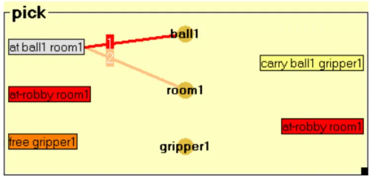
ViTAPlan (Visual Tool for Adaptive Planning) is an integrated environment for designing new planning problems, solving them and obtaining visual representations of the plans – solutions. The architecture of the visual tool, which is outlined in Figure 1, consists of the following sub-systems, which are discussed in more detail later in the chapter: a) designing, b) configuration, c) solving, d) visualizing and e) simulating.
HAP Problem Domain Execution Designing Simulating Visualizing Configuration Problem Analyzer Rule System ViTAPlan User
Figure 1. ViTAPlan's Architecture
The designing module provides visual representations of planning domains and problems through graphs that assist the user in comprehending their structure. Furthermore, the user is provided with graphical elements and tools for designing new domains and new problems over existing domains. This module communicates with the file system of the operating system, in order to save the designs in a planner – readable format (i.e. PDDL planning language) and also load and visualize past domains and problems.
The configuration module of ViTAPlan deals with the automatic fine-tuning of the planning parameters. This task is performed through two steps that are implemented in different sub-systems. The first one, called Problem Analyzer, reads the description of the problem from the input files, analyzes it and outputs a vector of numbers that correspond to the values of 35 measurable attributes that quantify the morphology of the problem in hand. The Rule System, which is consulted after the analysis of the problem, contains a number of rules that associate specific values or value ranges of the problems’ attributes with configurations of the planning parameters that guarantee good performance.
The execution module inputs the description of the problems (PDDL files of the domain and the problem) along with the values of the planner’s parameters and executes the planner (HAP or any other system attached to ViTAPlan) in order to obtain a solution (plan) to the problem. The planner’s parameters can be adjusted either by hand or automatically via the configuration module.
The last two sub-systems (visualization and simulation) present the plan that was inputted from the execution module in several forms. The visualization module presents the plan as a directed graph, through which the user can identify the positive and negative interactions among the actions and experiment with different orderings in which the plan’s steps should be executed. The second module simulates the problem’s world presenting all the intermediate states that occur after the execution of each action.
5. Visual Design of Planning Problems
The Design module of ViTAPlan serves as a tool for a) visualizing the structure of planning domains and problems in order to get a better understanding of their nature and b) designing new domains or new instances (problems) of existing domains with a user – friendly tool that can be used by non PDDL experts. The steps that a typical user must go through in order to design a new problem through ViTAPlan are the following: a) create the entity-relation model, b) design the operators, c) specify one or more problems, d) check the validity of the designs and e) translate the visual representations in PDDL language in order to solve the problem(s).
5.1. The Entity – Relation Model
The entities-relations diagram is a directed graph containing two types of nodes and one type of arcs connecting the nodes. The first type of nodes, called entity, is represented in the design as a circle and corresponds to an object class of the domain. The second type is represented by the visual tool as a rectangle and is used to specify relations between the domain’s classes. The edges connect rectangular with circular nodes and are used to specify which classes take part in each relation.
Consider the gripper domain for example, where there is a robot with N
grippers that moves in a space, composed of K rooms that are all connected with each
other. All the rooms are modeled as points and there are connections between each pair of points and therefore the robot is able to reach all rooms starting from any one of them with a simple movement. In the gripper domain there are L numbered balls
which the robot must carry from their initial position to their destination.
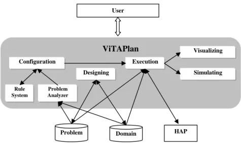
The diagram for the Gripper domain, which was used in the AIPS-98
planning competition, is illustrated in Figure 2. There are three object classes in the domain, namely room, ball and gripper that are represented with circles. There is no
class defined for the robot, since the domain assumes the presence of only one instance of it and therefore there is no need for an explicit definition.
The domain has four predicates: a) at-robby, which specifies the position of
the robot and it is connected only with one instance of room, b) at which specifies the
room in which each ball resides and therefore is connected with an instance of ball
and an instance of room, c) carry which defines the alternative position of a ball, i.e it
is hold by the robot and therefore it is connected with an instance of ball and an
instance of gripper and d) free which is connected only with an instance of gripper
and states that the current gripper does not hold any ball.
Note here that although PDDL, requires only the arity for each predicate and not the type of objects for the arguments, the interface obliges the user to connect each predicate with specific object classes and this is used for the consistency check of the domain design. According to the design of Figure 2, the arity of predicate
carry, for example, is two and the specific predicate can only be connected with one
object of class ball and one object of class gripper.
5.2. Representing Operators
The definition of operators in ViTAPlan follows a declarative schema, which is different from the classical STRIPS approach, although there is a direct way to transform definitions from one approach to the other. More specifically, an operator in the visual environment is represented with two lists, namely Pre and Post, that
contain the facts that must hold in a state S1in order to apply the operator and the facts that will be true in state S2 which will result from the application of the operator on S1 respectively. The relations between these lists and the three lists (Prec, Add, Del) of
the STRIPS notation are the following:
From STRIPS to ViTAPlan:
Post(A) = Add(A) ∪ (Prec(A) – Del(A)) From ViTAPlan to STRIPS:
Prec(A) = Pre(A) Add(A) = Post(A) - Pre(A) Del(A) = Pre(A) – Post(A)
Each operator in the interface is represented with a labeled frame, which contains a column of object classes in the middle, two columns of predicates on the two sides of it and connections between the object classes and the predicates. The un-grounded facts that are generated by the classes and the predicates in the left column define the Pre list of the operator while the Post list is defined by the predicates in the
right column.
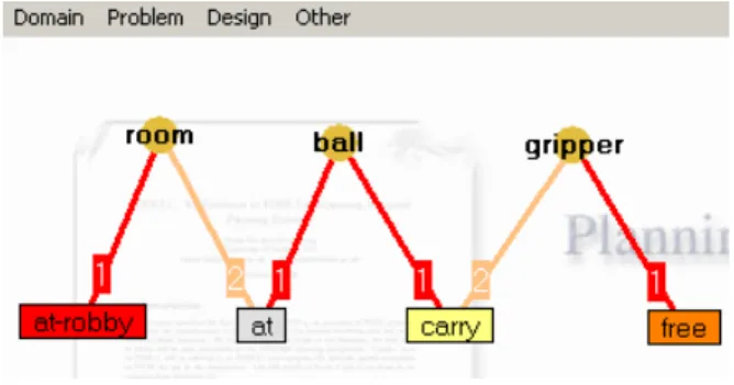
For example, in the gripper domain there are three operators: a) move which
allows the robot to move between rooms, b) pick which is used in order to lift a ball
using a gripper and c) drop which is the direct opposite of pick and is used to leave a
ball on the ground
The move operator is related with two instances of the room class (room1
and room2) which correspond to the initial and the destination room of the robot’s
move. The Pre and Post lists of the operator contain only one instance of the at-robby
relation. In the Pre list the at-robby is connected to room1, while thelatter is replaced
by room2 in the Post list. The definition of the move operator is presented in Figure 3.
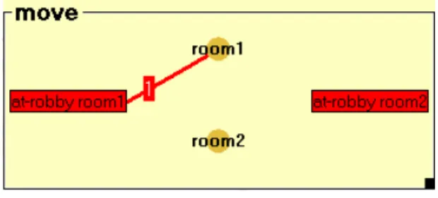
The second operator (pick), which is presented in Figure 4, contains one
instance from three entities, namely ball1, room1 and gripper1 that correspond to the
ball that resided on the room and was picked by a robot’s gripper. The Pre list defines
that both the ball and the robot must be in the same room and that the gripper must be free. The new fact that is contained in the Post list is that the gripper holds the ball,
while the freedom of the gripper and the fact that the ball resides on the room are deleted. The fact that the robot is in room1 is contained in both lists (Pre and Post)
since it is not deleted.
Figure 4. The pick operator
Similarly we define the drop operator which is presented in Figure 5. This
operator is the direct opposite of the pick operator and in fact it is produced by
exchanging the Prec and Post lists of the latter.
5.3. Representing Problems
The designing of problems in the interface follows a similar model with that of operators. Problems can be formed by creating a list of objects, two lists of predicates and a number of connections among them. The list which is created by the predicates in the left column and the objects corresponds to the initial state of the problem, while the goals are formed by the predicates of the right column.
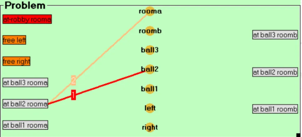
Figure 6 presents a problem of the gripper domain, which contains two rooms (rooma and roomb), three balls (ball1, ball2 και ball3) and the robot has two
grippers (left and right). The initial state of the problem defines the starting locations
of the robot and the balls and that both grippers are free. The goals specify the destinations of the three balls.
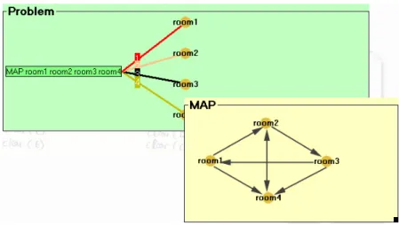
One of the key enhancements of ViTAPlan-2 over the past versions concerns the ability to use a predefined chain of objects that can be utilized for the definition of many kinds of facts. Consider for example the case where in gripper the moves of the robot are restricted by a relation (e.g. connected) which specifies which movements
are feasible. If we suppose that the map of the rooms is the one presented in Figure 7, then this would require the user to add the connected relation 7 times in the problem’s
definition and each time to make the appropriate connections (see Figure 8). This can become a severe problem for large and complex maps.
Figure 6. A Problem of the gripper domain
1
2
3
4
Figure 7. A map for a gripper problem
There is a number of cases where similar maps are required. For example in the hanoi domain, according to the definition adopted by the planning community, the
problem file must specify for each possible pair of pegs and discs which of the two is smaller. For a simple problem with three pegs and 5 discs, this yields 39 smaller relations.
In order to deal with this problem, ViTAPlan-2 contains a tool for building maps which makes it easier for the user to define multiple relations between pairs of objects that belong to the same entity. The user can use simple drag ‘n drop operations in order to define single and duplex connections between them. For example, the case described in Figure 8 can be easily encoded in ViTAPlan-2 using the map tool as shown in Figure 9.
Figure 9. The map tool
5.4. Syntax and Validity Checking
The visual environment besides the automation and the convenient way in which new domains and problems are designed, also performs a number of validity checks in the definitions, in order to assist the user in this really complex task. The entities-relations diagram, which is probably the most important part of the design of new domains is further used by ViTAPlan-2 as a reference model for the checks.
Each time the user tries to connect an instance of an entity E to an instance of a
i. This specific connection generates a fact that has already been defined in the same operator or in the problem. In this case the connection is rejected, since PDDL does not allow redefinitions of the same fact inside the same scope. ii. The definition of the relation in the entities-relations diagram contains a
connection to the entity in which E belongs.
iii. There is an empty slot in R which according to the diagram should be
connected to objects of the same class as that of E.
The checks listed above are also performed dynamically at each attempted change in the entities-relations diagram. For example, if the user deletes a connection between an entity and a relation, ViTAPlan will automatically delete any instance of this connection from all the operators and the definition of the problem. A similar update will also take place in the definition of the operators and in the problem, if the user deletes an entire relation or an entity.
Finally, a number of checks are also performed during the compilation of the design in PDDL. More specifically these checks contain:
• The case where no operator is defined
• The definition of empty operators
• The definition of void operators, i.e. operators with empty Pre and Post lists • The definition of effectless operators (Pre ≡Post)
• The definition of empty problems
• Semi-connected edges which lead to incomplete facts
5.5. Translation to PDDL
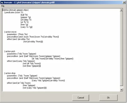
different planning systems. The environment contains a PDDL editor which enables the user to see and even modify the PDDL files of his designs. For example, the gripper domain and the specific problem used in this section are presented in Figure 10 and Figure 11 respectively.
Figure 10. The gripper domain in PDDL
6. System Configuration and Problem Solving
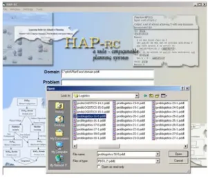
One of the main features of ViTAPlan is to allow the use of the underlying planning system in a friendlier and more accurate way. This interface between the user and the planning engine is carried out by the execution module of the visual environment. The inputs that must be supplied to the planning system are: a) the domain file, b) the problem file and c) the values of the planning parameters, in case of adjustable planners.
Figure 12. Selecting the input files
From the initial screen of the interface, which is shown in Figure 12, the user uses common dialogues and graphical elements in order to browse for the domain and problem files that will be inputted to the planner. From the same screen the user can also execute the planner and obtain the solution (plan), along with statistics concerning the execution, such as the planning time and the length of the plan. The way the results of the planner are presented to the user is shown in Figure 13.
Figure 13. Solving the problem
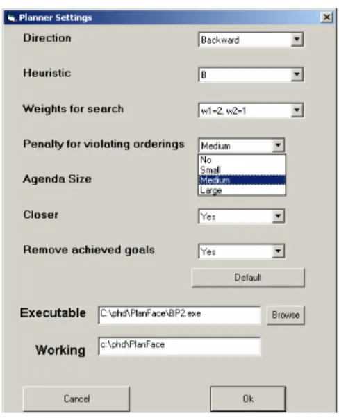
There are three ways for tuning the planner’s parameters in ViTAPlan: a) using the default values provided by the system, b) let the user assign the values by hand or c) use the configuration module in order to have the parameters set automatically. The user can select among the first two ways through the settings window presented in Figure 14. The parameters presented in this window correspond to the HAP planner which is embodied in ViTAPlan.
6.1. Hap planner
HAP, is a highly adjustable planning system that can be customized by the user through a number of parameters. These parameters concern the type of search, the quality of the heuristic and several other features that affect the planning process. The HAP system is based on the BP (Bi-directional Planner) planning system (Vrakas and Vlahavas 2002a) and uses an extended version of the ACE (Vrakas and Vlahavas 2002b) heuristic.
HAP is capable of planning in both directions (progression and regression). The system is quite symmetric and for each critical part of the planner, e.g. calculation of mutexes, discovery of goal orderings, computation of the heuristic, search strategies etc., there are implementations for both directions. The direction of
search is the first adjustable parameter of HAP used in tests, with the following values: a) 0 (Regression or Backward chaining) and b) 1 (Progression or Forward chaining).
As for the search itself, HAP adopts a weighted A* strategy with two independent weights: w1 for the estimated cost for reaching the final state and w2 for the accumulated cost of reaching the current state from the starting state (initial or goals depending on the selected direction). For the tests with HAP, we used four different assignments for the variable weights which correspond to different
assignments for w1 and w2: a) 0 (w1 =1, w2 =0), b) 1 (w1 =3, w2 =1), c) 2 (w1 =2, w2 =1) and d) 3 (w1=1, w2=1).
The size of the planning agenda (denoted as sof_agenda) of HAP also affects
the search strategy and it can also be set by the user. For example, if we set
sof_agenda to 1 and w2 to 0, the search algorithm becomes pure Hill-Climbing, while by setting sof_agenda to 1, w1 to 1 and w2 to 1 the search algorithm becomes A*.
Generally, by increasing the size of the agenda we reduce the risk of not finding a solution, even if at least one exists, while by reducing the size of the agenda the search algorithm becomes faster and we ensure that the planner will not run out of memory. For the tests we used three different settings for the size of the agenda: a) 1, b) 100 and c) 1000
The OB and OB-R functions introduced in BP and ACE respectively, are also
adopted by HAP in order to search the states of the search for violations of orderings between the facts of either the initial state or the goals, depending on the direction of the search. For each violation contained in a state, the estimated value of this state that is returned by the heuristic function, is increased by violation penalty, which is a constant number supplied by the user. For the experiments of this work we tested the HAP system with three different values of violation_penalty: a) 0, b) 10 and c) 100.
The HAP system employs the heuristic function of the ACE planner, plus two variations of it, which are in general more fine-grained. There are implementations of the heuristic functions for both planning directions. All the heuristic functions are constructed in a pre-planning phase by performing a relaxed search in the opposite direction of the one used in the search phase. During this relaxed search the heuristic function computes estimations for the distances of all grounded actions of the problem.
The user may select the heuristic function by configuring the heuristic_order
parameter. The three acceptable values are: a) 1 for the initial heuristic, b) 2 for the first variation and c) 3 for the second variation.
HAP also embodies a technique for simplifying the definition of the sub-problem in hand. This technique eliminates from the definition of the sub-sub-problem (current state and goals) all the goals that have already been achieved in the current
state and do not interfere in any way with the achievement of the remaining goals. In order to do this the technique performs, off-line before the search process, a dependency analysis on the goals of the problem. The parameter remove_subgoals is
used to turn on (value 1) and off (value 0) this feature of the planning system.
The last parameter of HAP is equal_estimation, which defines the way in
which states with the same estimated distances are treated. If equal_estimation is set
to 0 then between two states with the same value in the heuristic function, the one with the largest distance from the starting state (number of actions applied so far) is preferred. If equal_estimation is set to 1, then the search strategy will prefer the state,
which is closer to the starting state.
6.2. Configuration Module
The Configuration module of ViTAPlan is a sub-system able to adjust the planning parameters in an automatic manner. This feature is currently available only for use with the HAP planning system, although the methodology for the automatic configuration of planning parameters is general and can be applied to other planners as well (Tsoumakas et. al., 2004).
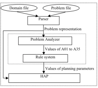
The automatic configuration is based on HAP-RC (Vrakas et. al., 2003), which uses a rule system in order to automatically select the best settings for each planning parameter, based on the morphology of the problem in hand. HAP-RC, whose architecture is outlined in Figure 15 is actually HAP with two additional modules (Problem Analyzer and Rule System) which are utilized off-line, just after reading the representation of the problem in order to fine tune the planning parameters of HAP.
Problem file Domain file Parser Problem Analyzer Rule system HAP Problem representation
Values of A01 to A35
Values of planning parameters
Figure 15. HAP-RC Architecture
The role of the Problem Analyzer is to identify the values of a specific set of 35 problem characteristics (noted as A1 to A35). These characteristics include measurable attributes of planning problems, such as number of facts per predicate and the branching factor of the problem, that present the internal structure of the problems in a quantified way. After the identification of the values of the attributes, which may require a limited search in the problem, the analyzer feeds the Rule system with a vector containing the values for the 35 problem attributes.
The Rule system contains a number of rules of the following format:
If preconditions list Then actions list
The preconditions of the rules check if the values of the problem’s attributes comply with some constraints on them, while the actions set one or more planning parameters to specific values. For example, the rule:
If A24<1.8 and A17<9.7 Then direction=1 and closer=yes
will trigger in a given problem if the values of A24 (ratio between the branching factors of the two directions) and A17 (standard deviation of the average number of actions deleting a fact) are smaller than 1.8 and 9.7 respectively. If this rule is
eventually fired, then the planning direction will be set to forward and the search algorithm will use the technique for overcoming plateaus.
What these rules actually do, is to propose setups for the planning parameters that worked efficiently in similar problems in the past. This knowledge has been extracted from Machine Learning techniques on data produced by thorough experiments with the HAP system. More specifically, we tested all the possible combinations of the parameters of HAP on a large set of problems from various domains and for each run we kept record of the values of the problem attributes, the specific setup for HAP and the value of a metric combining planning time and plan length. The data set was then fed to a Machine Learning tool in order to learn a rule-based classification model that would discriminate between good and bad values of the metric based on the rest of the attributes.
The Configuration module of ViTAPlan-2 also provides the user with the option to use the Problem Analyzer and the Rule System of HAP-RC in order to automatically fine-tune the planning parameters of HAP. The relevant window of the interface is shown in Figure 16. This window is divided in three parts: a) the first part shows the discretized values for the 35 problem characteristics, as produced by the Problem analyzer, b) the second part provides the user with the list of the rules that comprise the core knowledge of the system and c) the last part provides the user with the proposed values for the planning parameters of HAP.
The values of the problem’s attributes are presented in order to check for the triggered rules, but more importantly to assist the knowledge engineer or the domain expert in decoding the internal structure of the problem and extract useful insights from it. The tool presents the following information for each one of the 35 attributes: a) the code name (e.g A07), b) a description of the attribute (e.g. Standard deviation of
the number of facts per predicate), c) the arithmetic value, d) a discretized value (e.g. small) and e) the usual upper and lower limit for its value.
The rules are shown in the appropriate frame of the environment sorted by decreasing order of their confidence, as this was calculated by the learning algorithm. ViTAPlan presents all the rules, but the user is able to control the viewable part of the rules through two controls that select only the triggered rules or the rules that affect a specific parameter (e.g. heuristic function).
From the set of triggered rules, ViTAPlan makes an initial choice, selecting the rules with the highest confidence factor that are not in conflict with any other already selected rule. We say that two rules are in conflict, if they propose different setups for the same parameter. The configuration module uses the initial subset of selected rules in order to calculate the values of the parameters and present them to the user, leaving each unset parameter to its default value.
Figure 16. The rule system
Instead of just accepting or rejecting the proposed parameter setting, the user has the ability to interfere with the rule system, thus modifying the adopted conflict resolution strategy. More specifically, the user may either include a new rule in the
firing set, or request the removal of a selected one and thus alter the firing set and therefore the setup of the parameters. Each time the user requests the firing of a new rule Ri, the module automatically checks the resulting firing set for conflicts and
removes all the rules that propose contradictory values for the parameters affected by Ri.
Consider for example the case in Figure 17, which presents a portion of the triggered rules, i.e. those that require values for the attributes A01 to A35 that are compatible with the problem in hand. The initial selection contains rules 49, 74 and 154 that define the values 100, 2, 3 and 0 for the parameters penalty, heuristic, search_strategy
and direction respectively.
Figure 17. The initial firing set
Lets also suppose that the user requests rule number 35 (the first rule in Figure 17) to be included in the firing set. Rule 35 is in contradiction with rule 49, since the first sets penalty to 500 while the second sets it to 100 and with rule 154 for
the same reason. There is no contradiction with rule 74, since the only common parameter is heuristic and they propose the same value (2) for it. Therefore after the
inclusion of rule 35, rules 49 and 154 are removed from the firing set as shown in Figure 18. The proposed setup of the planner’s parameters becomes the following:
Figure 18. The final firing set
6.3. Embedding other planning systems
The current version of ViTAPlan embodies the HAP system, but the environment is open and the user can easily attach any other planner that reads the PDDL language. The communication protocol between the visual environment and the planner (including HAP) is outlined in Figure 19.
ViTAPlan-2 Environment
Planner
Domain
Problem Plan Pre-processor Description
Settings
Plan in X’s format
Plan in ViTAPlan’s format
Description
Figure 19. Communication with the planner
As already discussed the data that should be transmitted between ViTAPlan and the planning system are: a) the description of the domain and the problem, b) optionally the settings for the planner’s parameters and c) the plan that solves the problem.
Concerning the description of the problem, ViTAPlan is able to extract PDDL files, which is the standard definition language for all modern planners. Therefore it is trivial to submit the problem to any new planning system.
For each configurable parameter, ViTAPlan needs a description, the option used to set this parameter in the planner and the domain of values. This information must be specified by the user in order to add a new planner in the environment. The current version of ViTAPlan supports only discrete values for the domains of the parameters, but this can very easily be extended to support continuous values or other data types (e.g. booleans). For example, Table 1 presents part of the information that should be inputted to ViTAPlan-2 in order to connect it with the LPG planning system (Gerevini, Saetti and Serina, 2003).
Table 1. Specification of LPG’s parameters
Parameter Option Values
Heuristic identifier -h 1,2
Max number of restarts -restarts 1,2,3,4,5,6,7,8,9….
Nois
…
e added to Walksat -noise 0,0.1,0.2,0.3….
The output of any planner to a given problem is a sequence of actions that achieve the predefined goals. However, since there has not been a standard for describing plans yet, each planner may present the sequences of actions in a different way. Therefore a necessary step in order to attach a different planning system X on
ViTAPlan, is to format its output, either by modifying the system, or by adding a pre-processor that reads the plan in X’s format and transforms it. Figure 20 presents an
example of a plan in ViTAPlan’s format.
3: (load hoist1 crate0 truck0 distributor0) 2: (lift hoist1 crate0 pallet1 distributor0) 1: (drive truck0 distributor1 distributor0) Begin of Plan
7. Plan Representations
There are two modules for visualizing the plans in ViTAPlan: the execution simulation which simulates the execution of the plan in a virtual world and the steps visualization that presents the plan as an action graph.
7.1. World Simulation
This module of ViTAPlan allows the user to execute the plan that was acquired from the execution sub system and trace the changes that occur to the world as the actions of the plan are sequentially applied. Figure 21 presents the simulation module, which consists of three parts. The first one is a scroll bar, through which the user can browse for a specific action of the plan. The other two parts present the states of the world before the application of the selected action (left part) and after it (right part) respectively.
Figure 21. Execution simulation
In the example presented in Figure 21 the first action of the plan is selected and therefore the state presented in the left part is the initial one, while the one in the right part is the first intermediate state. The tool uses proper color coding in order to discriminate the facts in four categories:
i. facts of the preceding state that are deleted by the action ii. new facts that are added to the new state
iii. propagated facts iv. static facts
7.2. Graph based Representations
The second option for the user is to view the actions of the plan on a timeline, as shown in Figure 22. The timeline for the plan presents for each action the point in which it is scheduled to be executed and the facts in its precondition and add lists. Moreover, the visualization shows the interactions between the actions in the plan. More specifically, for each action A the user is able to see connections between:
i. each precondition of A and the most recent action that achieved it
ii. each fact that is deleted by A and the most recent action that established it
iii. each fact that is added by A and the following actions that have it in their
preconditions
Figure 22. Step graph
The connections represented by the arcs in the graph present in graphical way all the interactions (positive and negative) between the steps of the plan and therefore allow the user to:
i. Comprehend the specific sorting in which the steps have been ordered and why a specific action should be placed before (or after) another one.
ii. Replace an action or a set of actions with other, taking care so as not to violate the interactions, and thus produce modified or alternative plans.
iii. Find parallelizations in the plan execution and therefore reduce the total execution time and the cost of its application.
8. Conclusion and Future Work
This chapter presented ViTAPlan, a unified environment for automated planning which contains several modules with user friendly interfaces. The main feature of the environment is the designing module which saves the user from the strict syntax of the Planning Domain Definition Language (PDDL). The user is able to visualize and design new domains and problems in an easy-to-use graphical way and the tool is responsible for checking the validity of the designs and translating them in PDDL files.
The current version of the environment has four main functions: a) using the planning system through a number of windows, controls and common dialogues, which makes it much easier for a non – programmer to use the planner and experiment with different setups of the planning parameters, b) use the Problem Analyzer and the Rule System of HAP-RC in order to acquire useful knowledge about the morphology of each problem and automatically fine tune the planner with the most appropriate values for the planning parameters c) generating new domains and problems using a visual tool and d) produce visual representations of the plans found by the planning system, which enable the user to better understand each step in the plan and also intervene and alter the plan at will.
In the future, we plan to improve the interface in all functions of it and introduce others that will make it a complete tool for planning both for academic and industrial use. It is in our direct plans to enhance the tool for designing domains and problems with the ability to handle advanced aspects of the latest versions of PDDL, such as treatment of numerical values, explicit representation of time and duration, conditional effects e.t.c.
In parallel, we are currently working on developing an interface for ViTAPlan in order to input OWL-S documents that describe simple or complex Semantic Web Services and automatically translate them to PDDL problem definitions. Then, our visual tool will enable authoring of appropriate service composition operators as planning operators that will solve the Semantic Web Service composition problem. The Produced plan will constitute the complex Web Service and it will be exported in an appropriate Web Service choreography language or in OWL-S to a corresponding complex Web Service execution monitoring tool or it will be just published at a UDDI registry.
References
1. Aalst W. van der, "Don't Go with the Flow: Web Services Composition Standards Exposed", IEEE Intelligent Systems, Vol. 18, No. 1, pp. 72-76, 2003.
2. Berardi D., Calvanese D., De Giacomo G., Mecella M., "Reasoning about Actions for e-Service Composition", ICAPS 2003 Workshop on Planning for Web Services.
3. Berners-Lee T., Hendler J., and Lassila O., “The Semantic Web”, Scientific American, 284(5), 2001, pp. 34-43.
4. Blum, A., and Furst, M., Fast planning through planning graph analysis, In
Proceedings of the 14th International Conference on Artificial Intelligence,
5. Blythe J., Deelman E., Gil Y., "Planning for workflow construction and maintenance on the Grid", ICAPS 2003 Workshop on Planning for Web Services.
6. Bonet, B. and Geffner, H., Planning as Heuristic Search. Artificial Intelligence, Special issue on Heuristic Search, 129/1-2 (2001), 5-33.
7. Booth D. et al., "Web Services Architecture", W3C Working Draft, Aug. 2003. http://www.w3.org/TR/ws-arch/
8. Botea, A., Enzenberger, M., Müller, M. and Schaeffer, J., Macro-FF: Improving AI Planning with Automatically Learned Macro-Operators, To appear in Journal of Artificial Intelligence Research (2005).
9. Bourbakis, N. and Tascillo, A., An SPN-Neural Planning Methodology for Coordination of two Robotic Hands with Constrained Placement, Journal of Intelligent and Robotic Systems archive, 19-3 (1997), 321-337,
10. Carman M., Serafini L., Traverso P., "Web Service Composition as Planning",
ICAPS 2003 Workshop on Planning for Web Services.
11. Chen, Y., Wah, B. W. and Hsu, C., Subgoal Partitioning and Resolution for Temporal Planning in SGPlan, Journal of Artificial Intelligence Research
(2005).
12. Edelkamp, S. and Hoffmann, J., PDDL 2.2: The Language for the Classical Part
of IPC-4, in Proceedings of the International Planning Competition
International Conference on Automated Planning and Scheduling (Whistler
2004), 1-7.
13. Fikes, R. and Nilsson, N. J., STRIPS: A new approach to the application of theorem proving to problem solving, Artificial Intelligence, Vol 2 (1971),
189-208.
14. Fox, M. and Long, D., PDDL2.1: An extension to PDDL for expressing
temporal planning domains. Journal of Artificial Intelligence Research, 20
(2003), 61-124.
15. Friedman-Hill, E. J., "Jess, The Expert System Shell for the Java Platform", 2002, http://herzberg.ca.sandia.gov/jess/
16. Gerevini, A., Saetti, A. and Serina, I., Planning through Stochastic Local Search and Temporal Action Graphs. Journal of Artificial Intelligence Research, 20
(2003), 239-290.
17. Gerevini, A., Saetti, A. and Serina, I., Planning in PDDL2.2 Domains with LPG-TD, in International Planning Competition, 14th Int. Conference on Automated Planning and Scheduling (ICAPS-04), abstract booklet of the competing planners, (2004).
18. Gerevini, A. and Long, D., Plan Constraints and Preferences in PDDL3,
Technical Report R.T. 2005-08-47, Dipartimento di Elettronica per
l’Automazione, Università degli Studi di Brescia, via Branze 38, 25123 Brescia, Italy.
19. Ghallab, M., Howe, A., Knoblock, C., McDermott, D., Ram, A., Veloso, M., Weld, D. and Wilkins, D., PDDL -- the planning domain definition language.