Liquidity Mergers

NBER WORKING PAPER SERIES

LIQUIDITY MERGERS

Heitor Almeida

Murillo Campello

Dirk Hackbarth

Working Paper 16724

http://www.nber.org/papers/w16724

NATIONAL BUREAU OF ECONOMIC RESEARCH

1050 Massachusetts Avenue

Cambridge, MA 02138

January 2011

We thank Todd Gormley (AFA discussant), Charles Hadlock, Jerry Hoberg, Hernan Ortiz-Molina,

Gordon Phillips, Michael Schill (EFA discussant), Erik Theissen, and an anonymous referee for their

detailed comments and suggestions. Comments from audiences at the 2010 AFA Meetings, the 2010

EFA Meetings, ESMTBerlin, Michigan State University, MIT, Simon Fraser University, University

of British Columbia, University of Mannheim, University of Michigan, University of Utah, and Vienna

University are also appreciated. Lifeng Gu and Fabrício D’Almeida provided excellent research assistance.

The views expressed herein are those of the authors and do not necessarily reflect the views of the

National Bureau of Economic Research.

NBER working papers are circulated for discussion and comment purposes. They have not been

peer-reviewed or been subject to the review by the NBER Board of Directors that accompanies official

NBER publications.

Liquidity Mergers

Heitor Almeida, Murillo Campello, and Dirk Hackbarth

NBER Working Paper No. 16724

January 2011

JEL No. G31,G32,G33,G34

ABSTRACT

We study the interplay between corporate liquidity and asset reallocation opportunities. Our model

shows that financially distressed firms are acquired by liquid firms in their industries even when there

are no operational synergies associated with the merger. We call these transactions “liquidity mergers,”

since their main purpose is to reallocate liquidity to firms that might be otherwise inefficiently terminated.

We show that liquidity mergers are more likely to occur when industry-level asset specificity is high

(i.e., industry-specific rents are high) and firm-level asset specificity is low (industry counterparts

can efficiently operate distressed firms’ assets). We also provide a detailed analysis of firms’ liquidity

policies as a function of real asset reallocation, examining the trade-offs between cash and lines of

credit. The model makes a number of predictions that have not been examined in the literature. Using

a large sample of mergers, we verify the model’s prediction that liquidity-driven acquisitions are more

likely to occur in industries in which assets are industry-specific, but transferable across industry rival

firms. We also verify the prediction that firms are more likely to use credit lines (relative to cash) when

they operate in industries in which liquidity mergers are more frequent.

Heitor Almeida

University of Illinois at Urbana-Champaign

515 East Gregory Drive, 4037 BIF

Champaign, IL, 61820

and NBER

[email protected]

Murillo Campello

University of Illinois at Urbana Champaign

4039 BIF

515 East Gregory Drive, MC- 520

Champaign, IL 61820

and NBER

[email protected]

Dirk Hackbarth

University of Illinois at Urbana-Champaign

515 East Gregory Drive, 4035 BIF

1206 S. Sixth Street

Champaign, IL 61820

[email protected]

1.

Introduction

Existing research argues investment funding is a key determinant of corporate liquidity policies (see, e.g., Opler et al. (1999), Graham and Harvey (2001), Almeida et al. (2004), and Denis and Sibilikov (2010)). Given that acquisitions are one of the most important forms of investment, one would expect that the benefits and costs of asset reallocation would be an important driver of liquidity. However, this notion has been largely overlooked by the literature on corporate liquidity.

In this paper, we propose and develop a theoretical link between corporate liquidity policies and asset reallocation opportunities. Our model explains why a distressed firm might be acquired by a liquid firm in its industry even when there are no true operational synergies between the firms.1 We call this type of acquisition aliquidity merger. The model adds to our understanding of liquidity man-agement by showing how credit lines might dominate alternatives such as cash and ex-post financing in the funding of acquisitions. In particular, it shows that credit lines can be a particularly attractive source of liquidity for high net worth, profitable firms.

The model’s basic argument is as follows. Consider a firm that finds it difficult to raise credit because it cannot pledge its cash flows to investors. Limited pledgeability can arise from many sources, including moral hazard, asymmetric information, or private control benefits. In the model, firm insiders derive a non-pledgeable rent from their ability to manage assets that are industry-specific. If thefirm is hit by a liquidity shock that is larger than its pledgeable value, thefirm might not be able to raise the extra capital it needs even if continuation would be efficient. One option is to liquidate the distressed firm’s assets at the value that can be captured by industry outsiders (“sell for scrap”). But if other industry players are able to operate the industry-specific assets (“putting those assets to uses they were designed for”), an acquisition by a healthy industry rival may dominate liquidation.2 The problem with that alternative is that the acquirer itself may end up facing a similar pledgeability problem. In particular, outside investors (including those of the acquirer) might be unwilling tofinance the merger since they can only capture the pledgeable portion of the gains associated with the deal.

How can the industry acquirer overcome this financing problem? To do this, the acquirer needs a source of funding that can be used at its discretion. The situation resembles the ex-ante liquidity insurance problem of Holmstrom and Tirole (1997, 1998). In the Holmstrom-Tirole framework, the firm cannot wait to borrow after a large liquidity shock is realized because at that point external

1_{By “lack of true operational synergies” we mean that a merger between thefirms would not increase their combined}

value in the absence of financial distress. We do not imply that mergers do not generate operational synergies, but simply that they might occur even in the absence of such synergies. See Maksimovic and Phillips (2001) for evidence on productivity gains arising from mergers.

2_{Consistent with this notion, Ortiz-Molina and Phillips (2009)find that inside liquidity (provided by buyers inside}

investors would be unwilling to provide funds. Instead, the firm needs to contract its financing ex-ante. The optimal liquidity policy can be implemented either in terms of cash (the firm borrows more than its ex-ante needs) or with an irrevocable line of credit. A similar logic follows through in the financing of a liquidity merger. The industry acquirer can overcome investors’ unwillingness

tofinance the merger by accessing a discretionary form of financing that does not require investors’

ex-post approval. Liquidity mergers thus emerge as a link between firm financial policies and asset reallocation opportunities in an industry.3

Putting our theory in perspective, we model the link between mergers and liquidity policy by em-bedding the Holmstrom and Tirole (1997, 1998) liquidity demand model in an industry equilibrium framework that draws on Shleifer and Vishny (1992). Previous research suggests that a practical problem with lines of credit is that they may become unavailable precisely when thefirm most needs them. However, the industry acquirer is most likely to demand liquidity for an acquisition in states in which it does not suffer a negative liquidity shock of its own. Hence covenants that link line of credit availability to thefirm’s cashflow performance need not restrict the availability offinancing to acquirers. We use this insight to show that lines of credit might dominate cash infinancing liquidity-driven mergers, even when those credit facilities are revocable. In order to use cash tofinance future acquisitions, the acquirer would need to carry large balances from the current period to all future states of the world. In the presence of a liquidity premium, this policy is costly. Given that cash

flow-based covenants do not restrict the availability of merger financing under the credit line, cash

becomes less desirable as the demand for mergerfinancing increases.4 The model analysis shows how merger activity may influence whetherfirms use cash or credit lines in their liquidity management. The analysis is novel, among other reasons, because it helps reconcile the observed positive correlation between afirm’s profitability and its use of credit lines in lieu of cash for liquidity management (see Sufi (2009) and Campello et al. (2010)).

Our model has several implications that have not yet been examined in the literature. First, it predicts that liquidity mergers should be more frequent in industries with high asset specificity, but amongfirms whose assets are not toofirm-specific. We identify these industries empirically based on two observations. First, we conjecture that industry-specificity is likely to be greater for assets such as machinery and equipment than for land and buildings. Accordingly, we use the ratio of machinery and equipment to total firm assets as a proxy for industry asset specificity (“machinery intensity”). Second, we conjecture that firm-specificity should be inversely related to the degree of activity in

3

Industry peers are unique liquidity providers in the Holmstrom-Tirole setup because unlike industry outsiders (e.g., buyout groups) their management can capture non-pledgeable income associated with the assets of distressed targets.

4_{As we discuss below, the credit line reduces liquidity premia since it does not require thefirm (nor the lender) to}

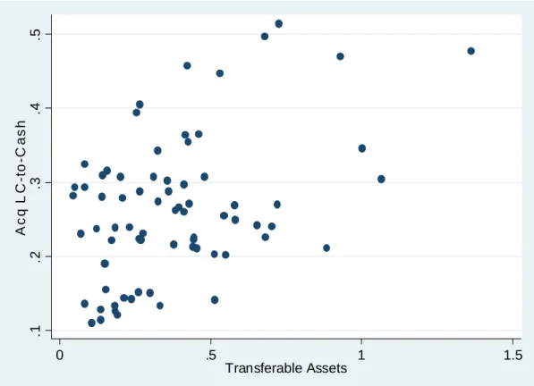
asset resale market in a firm’s industry – the higher the use of second-hand capital amongst firms in an industry, the lessfirm-specific the capital. To construct a measure of “capital salability” within an industry, we hand collect data for used and new capital acquisitions from the Bureau of Census’ Economic Census. These data allow us to gauge asset salability through the ratio of used to total (i.e., used plus new)fixed capital expenditures byfirms in an industry (cf. Almeida and Campello (2007)). Combining those two observations, we construct our desired measure as the product of “machinery intensity” and “capital salability.” We call this composite proxy Transferable Assets.

We then investigate if the ratio of liquidity mergers to the total number of mergers in an industry is related to asset specificity (Transferable Assets). Using a sample of 1,097 same-industry mergers drawn from the SDC database between 1980 and 2006, we identify deals as potential liquidity mergers as those in which the target is arguably close tofinancial distress. Specifically, we attempt to isolate targets that have lower interest coverage than the average target, but at the same time have high profitability (to alleviate concerns that the target firm may be economically distressed). Our tests include cross-industry regressions that control for characteristics such as industry-wide measures of

financial distress, concentration, and capacity utilization. Consistent with our theory, we find

evi-dence that the likelihood of liquidity mergers is higher when assets are both highly industry-specific and easily redeployable amongst industry rivals.5

In addition to our baseline test, we also examine the likelihood of same-industry acquisitions of distressed targets in the aftermath of a liquidity shock. To do this, we examine the collapse of the junk bond market in the late 1980s. A number of developments taking place in 1989 effectively meant that junk-bond issuers lost access to liquidity coming from the corporate bond market – they experienced an exogenous shock to the supply of credit (see also Lemmon and Roberts (2010)). We study the patterns of liquidity-driven acquisitions involving thefirms that were affected by this pointed liquidity shock. These additional tests confirm our model’s prediction that, when faced with liquidity shocks,

firms may engage in merger deals in which their assets are transferred towards other firms in their

same industry depending on the level of asset specificity.

The second model implication that we examine is thatfirms are more likely to use credit lines for liquidity management if industry asset-specificity is high, but firm asset-specificity is low (i.e., when Transferable Assets is high). We use two alternative data sources to test this implication. Ourfirst sample consists of a large data set of loan initiations drawn from the LPC-DealScan over the 1987—2008 period. The LPC-DealScan data have two potential drawbacks, nonetheless. First, they are largely based on syndicated loans, thus biased towards large deals (consequently largefirms). Second, they do

5

We alsofind that the fraction of liquidity-driven deals in our sample ofintra-industrymergers is significantly higher than the fraction of liquidity-driven deals in a sample ofinter-industry mergers. Thisfinding supports our contention that industryfirms are natural suppliers of liquidity for distressed rivals.

not reveal the extent to which existing lines have been used (drawdowns). To overcome these issues, we also use an alternative sample that contains detailed information on the credit lines initiated and used by a random sample of 300firms between 1996 and 2003. These data are drawn from Sufi(2009). We measure the use of credit lines in corporate liquidity management by computing the ratio of available credit lines to available credit lines plus cash holdings. Our panel regressions show thatfirms are more likely to use credit lines in their liquidity management (relative to cash holdings) if they operate in industries with specific but transferable assets. This result is statistically and economically significant. For example, when using Sufi’s (2009) sample we find that a one-standard deviation in-crease inTransferable Assetsincreases the ratio of credit lines to total liquidity by0.10, approximately 20% of the mean value of this ratio. This result is consistent with the model’s implication that lines of credit are an attractive way tofinance growth opportunities such as liquidity-driven acquisitions.6 Existing survey evidence suggests that lines of credit are not only used for liquidity management, but also to fund real operations (see Campello et al. (2010)). CFOs also indicate that credit lines are used tofinance growth opportunities (such as acquisitions), while cash is used to withstand negative liquidity shocks (Lins et al. (2010)). To our knowledge, this is thefirst paper that theoretically recon-ciles real-world managers’ view that cash and lines of credit are used for different purposes. A recent paper by Gabudean (2007) analyzes the interplay among rivals’ cash policies in a Shleifer-Vishny industry equilibrium, but it does not examine liquidity mergers nor the trade-off between cash and credit lines. Asvanunt et al. (2007) show that cash holdings may be dominated by an adequately de-signed line of credit policy. Our paper, however, is thefirst to model the role of alternative liquidity instruments in thefinancing of acquisitions.7

Recent empirical papers examine the effect of excess cash on acquisitions (e.g., Harford (1999), Dittmar and Mahrt-Smith (2007), and Harford et al. (2008)). While their evidence also motivates our analysis, we focus on the opposite direction of causality. Namely, we model how the anticipation of acquisition opportunities affects corporate liquidity policy. In this sense, our paper is closer to Harford et al. (2009), who look at how deviations from target leverage affect whether acquisitions are financed with debt or equity. The key difference is that we focus on liquidity policy variables rather than leverage ratios. Our paper is also related to previous studies that analyze conglomerate mergers as a way of dealing with the target’s inability to raise external funds (e.g., Hubbard and Palia (1999), Fluck and Lynch (1999), Inderst and Mueller (2003)).8 One distinguishing feature of our merger

6_{We further discuss aggregate statistics and anecdotal evidence supporting our model’s intuition that lines of credit}

are frequently used in the real-world tofinance liquidity mergers.

7_{Maksimovic (1990) shows that credit lines can boost a firm’s competitive position in an imperfectly competitive}

industry, but the author does not analyze the trade-offbetween cash and credit lines.

8_{Maksimovic and Phillips (2002) consider an alternative neoclassical model of conglomerate mergers that rely on}

model is that it pertains to within-industry acquisitions, as opposed to diversifying mergers. On a more theoretical level, we note that in prior models mergers help mitigate the friction that generates the target’sfinancial distress and increase the target’s externalfinancing capacity.9 However, it is not the case that the acquirer directly supplies liquidity to the target as in our model, nor there is a clear role for the acquirer’s liquidity policy.

The model we propose is novel in showing that acquirers from inside the industry are unique in turning around distressed assets. In particular, managers of rival firms are special in that their expertise allows them to extract asset-specific benefits from assets commonly used in their industry (“transferable assets”). Those agents mayboth gainfully operate distressed assets in the industry and bring to the table the funds needed to remedy liquidity shocks; funds that are made available immedi-ately by virtue of pre-committedfinancing arrangements. In this way, credit line-financed rivals have the necessary liquidity and ability to turn around distressedfirms – they are unique in implementing a liquidity merger. Our model and empirics contribute to the literature by characterizing a situation in which liquidity constraints are resolved by a well-characterized combination offinancial contracting and human capital expertise.

Finally, while the link between liquidity mergers and credit lines underlies our analysis, we stress that a central contribution of our work is to demonstrate the more general idea that credit lines are an effective way to transfer liquidity across states. Our point about credit lines is that they are a particularly effective way tofinance investment opportunities that arrive in good states of the world, and for which thefirm needs internal liquidity. While a “liquidity merger” strikes us as an interesting, practical example of such investments, it is certainly not the only one. Notably, however, it would be more difficult to test the model’s predictions by looking at general investment items, such as capital expenditures. This is so because it is difficult to empirically isolate capital expenses that satisfy the model’s conditions for a credit line to be an effective liquidity management tool (e.g., they need to arrive in good states of the world and strictly require internal liquidity). Similarly, the key economic insight behind the liquidity merger story is the advantage that the industry acquirer has in liquidity provision to distressed rivals. Whether the acquirer can supply liquidity to distressedfirms depends on whether the acquirer has enough committed liquidity to draw on, and not on whether the liquidity comes strictly from credit lines.

In the next section we develop the benchmark model of liquidity demand and liquidity mergers. We do so under a security-design framework in whichfirms choose their optimal liquidity demand (at first) without any implementation constraints. The implementation of optimal liquidity using cash and credit lines is discussed in Section 3. Section 4 introduces a number of extensions to the basic

9

model. Section 5 discusses the model’s main empirical implications. The model’s predictions are tested in Section 6. Section 7 concludes the paper. All proofs are placed in the Appendix.

2.

A model of liquidity mergers and liquidity demand

We start from Holmstrom and Tirole’s (1997, 1998) model of corporate liquidity demand, and embed

thefirm’s liquidity optimization problem in an industry equilibrium that follows Shleifer and Vishny

(1992). While these two theoretical pieces are well known, their insights have not been brought up together as a way to rationalizefirm liquidity policy as a function of merger activity.

2.1.

Basic framework

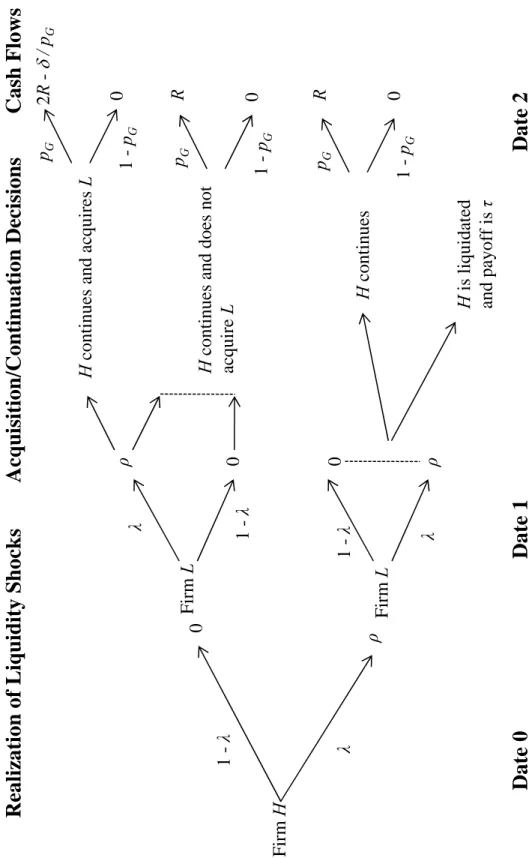
Consider an industry with twofirms, which we callHandL.10 There are three dates, and no discount-ing. Bothfirms have an investment opportunity offixed sizeI at date 0. Thefirms differ according to their date-0 wealth,A. FirmH is a high wealthfirm, so thatAH > AL. The investment opportunity also requires an additional investment at date 1, of uncertain size. This additional investment repre-sents thefirms’ liquidity need at date 1. We assume that the date 1 investment can be either equal to ρ, with probabilityλ, or0, with probability(1₋λ). For now, we take that the investment need is i.i.d. acrossfirms, that is, the probability thatfirmHdraws ρis independent of whetherfirmLdrawsρor 0. We refer to states using probabilities. So, for example, stateλ2 is the state in which bothfirms have date 1 investment needs. For convention, we letλ(1₋λ)be the state in which onlyfirmH has a liq-uidity need for investment, and(1₋λ)λbe the state in which onlyfirmLhas a date 1 liquidity need.11 Afirm will only continue its date 0 investment until date 2 if it can meet the date 1 liquidity need. If the firm continues, the investment produces a date-2 cash flowR which obtains with probability p. With probability 1₋p the investment produces nothing. The probability of success depends on the input of specific human capital by the firms’ managers. If the managers exert high effort, the probability of success is equal to pG. If effort is low, the probability of success is lower, equal to pB; however, managers consume a private benefit equal to B. Because of the private benefit, managers must keep a high enough stake in the project to induce effort. We assume that the investment is negative NPV if the managers do not exert effort, implying the following incentive constraint:

pGRM _≥ pBRM +B, or (1) RM ≥

B

∆p,

1 0_{In Section 4 we consider an extension in which there are manyfirms of each type.} 1 1

In Section 4 we consider, among other extensions, positively correlated investment needs and continuously distributed liquidity shocks.

whereRM is the managers’ compensation and∆p=pG−pB. This moral hazard problem implies that

the firms’ cash flows cannot be pledged in their entirety to outside investors. Following Holmstrom

and Tirole, we define:

ρ_{0 ≡}pG(R− B

∆p)< ρ1 ≡pGR. (2) The parameter ρ₀ represents the investment’s pledgeable income, and ρ₁ its total expected payoff. Using moral hazard to generate limited pledgeability greatly improves the model’s tractability. How-ever, we stress that this interpretation does not need to be taken literally. For example, our model’s central results would carry through if limited pledgeability was generated by information frictions betweenfirm insiders and outside investors.

If the firm cannot meet the liquidity need, it is liquidated generating an exogenous payoff that does not rely on industry-specific managerial human capital (and thus is fully pledgeable to outside investors). We let this liquidation value be equal toτ < I. In the current model, liquidation should be interpreted as the value of thefirm’s assets to an “outsider,” that is, an investor who does not possess industry-specific human capital. The higher the τ, the lower is the industry-specificity of the firm’s assets. We assume that the project is positive NPV, even if it needs to be liquidated in state(1₋λ): U = (1₋λ)ρ₁+λτ₋I >0. (3) In lieu of liquidation, afirm that cannot meet its liquidity need can try to sell its assets to another

firm in the industry. Since managers of other industry firms have industry-specific human capital,

they may be able to generate higher value from the assets. However, because human capital may have a firm-specific component, industry managers are not perfect substitutes for each other. We assume that an industry manager can produce a cashflowR_−pGδ by operating the assets of another industry firm.12 The parameterδcaptures the extent to which industry assets arefirm-specific. For simplicity, we assume that the buyer of the assets always makes a take-it-or-leave-it offer to the distressed seller, meaning that the transaction price is always equal to the seller’s outside option (τ).13

Figure 1 About Here

Figure 1 shows the model’s time line and summarizes the sequence of actions from the perspective of firm H. The figure also includes the realizations of liquidity shocks affectingfirm L to show how the actions of firm H depend on whether firm L is in distress. To simplify the tree, we assume that firmH will only bid forfirmLin the state in whichfirmH does not have tofinance its own liquidity shock (i.e., state(1₋λ)). As we show below, this is a natural outcome of the model. In addition, the

1 2

The probability of success and the private benefit are assumed to be the same as in the originalfirm. Thus, the asset generates date-1 pledgeable income equal toρ₀₋δif it is reallocated acrossfirms.

1 3

tree incorporates the fact that managers must exert high effort on the equilibrium path and hence the probability of success at date 2 is always equal topG.

2.1.1. Assumptions about pledgeability and net worth

We make the following assumptions about the model parameters:

ρ₀< ρ < ρ₁₋τ. (4) Given that a liquidity shock occurs, the net benefit of continuation isρ₁₋τ. This assumption means that it is optimal for the firms to withstand the liquidity shock, but that date-1 pledgeable income is not sufficient tofinance the shock. The model becomes trivial if this assumption does not hold, in that firms will generally not need liquidity insurance (if ρ_{0 ≥}ρ), or that it will never be optimal to survive a liquidity shock or to bid for the other industryfirm (if ρ_≥ρ₁₋τ).

We make the following assumption about AL:

ρ₀₋λρ < I₋AL≤(1−λ)ρ0+λτ. (5)

This implies thatfirmLdoes not have enough pledgeable income to be able to meet the liquidity need ρin stateλ. However, iffirmL is liquidated in stateλ, it generates total expected date 0 pledgeable income of(1₋λ)ρ₀+λτ, which by (5) is larger thanI₋AL. This assumption allows us to focus on the most interesting case in whichfirmLinvests at date0and may become a target forfirmHat date 1. In this three-period model, thefirm’s “wealth level”Ais a quantity that summarizes thefirm’s re-cent history, in particular the cumulative effects of past cashflow innovations. Assumption 5 captures the possibility that some industry firms may have, at some point in time, low enough accumulated wealth that they cannot fund future liquidity shocks on their own. Despite having low liquidity, firms of typeLretain profitable investment opportunities. Specifically, condition 4 says thatfirmL’s assets produce greater value under continuation (ρ₁₋ρ) than liquidation (τ). Thus,firmLfaces the potential of financial distress if a liquidity shock hits at date 1.

We make the following assumption about AH:

ρ₀₋2λρ₋λ[τ₋(ρ₀₋δ)]< I₋AH _≤ρ₀₋λρ₋(1₋λ)λ[ρ+τ ₋(ρ₀₋δ)]. (6) This assumption ensures thatfirmH has enough pledgeable income to withstand the liquidity shock and also bid for firm L in the case firm L is in distress. However, pledgeable income is enough to

finance H’s bid only in the event that H itself does not have a liquidity need in date 1. The role of

this assumption will become clearer below. It captures the idea thatfirmH will be most likely to bid forL if its internal liquidity is high, which will happen in the case thatH does not suffer a liquidity shock. Clearly, if firm H never has enough pledgeable income to to bid for firm L there will be no interactions amongfirms in the model.

2.1.2. External financing and liquidity insurance

Firms raise funds from external investors to finance the date-0 investment I, the date-1 investment ρ (when it is required), and also the bid for other industry firms that might become distressed. Throughout, we make the usual assumption that contracts are structured such that investors break even from the perspective of date 0.

In order to characterize the best possible financial contract that firms can get, we first take a security-design approach. Specifically, we assume thatfirms can write state-contingent contracts with external investors that specify the amount of payments that are made in each state of the world at date 1 and date 2. In Section 3, we will implement this optimal contract using real-world securities (such as cash and credit lines). This solution method helps highlight the trade-offbetween cash and credit lines by comparing them against a benchmark of perfect state-contingent contracts.

In addition to date-1 payments, the optimal date-0 contract specifies the amount of external fi-nance thatfirms raise at date 0, and the promised payment in case of success at date 2 (which happens with probability pG). We denote the contractual amounts by (K0, K1,s, K2,s), where s denotes the

state of nature that realizes at date 1 (for example,λ(1₋λ)).14

These contractual amounts must satisfy feasibility and pledgeability constraints. For each firm j we must have that K0 ≥ I −Aj, so that firms have enough funds to start their projects. The constraints thatK1,s must meet depend on the investment strategy that firms wish to implement at date 1. For example, in order for firms to withstand the liquidity shock in state λ it must be the case that K1,λ ≥ρ. For a firm to be able to bid for the other firm in state (1−λ)λ, we must have K_{1,(1−λ)λ ≥}ρ+τ, so that the acquirer can cover the target’s liquidity shock and liquidation option. The date-2 promised payments must obey the pledgeability constraints. In states in which a firm continues but does not acquire other assets, we must have ₋K2,s ≤ R− _∆B_p (or −pGK2,s ≤ ρ0). If

a firm acquires the other one in state (1₋λ)λ, we must have ₋pGK2,(1−λ)λ ≤2ρ0−δ. Finally, the

payments(K0, K1,s, K2,s) must be set such that investors break even from the perspective of date 0.

2.2.

Equilibria

In equilibrium, firms choose their optimal investment andfinancing policies taking into account the optimal actions of the otherfirm. The model generates two different equilibria, depending on whether a liquidity merger is profitable or not. The liquidity merger is not profitable if:

ρ₁₋δ < ρ+τ. (7)

1 4

Sincefirms produce zero cashflows in case of failure at date 2, the realization of uncertainty at date 2 is irrelevant. Firms promise payments out of date-2 cashflows, which are made only in the case of success.

Firm H can generate a date-1 expected payoffof ρ₁₋δ by operating the assets offirm L. However, the merger requires firmH to coverL’s liquidity shock and compensateL’s investors, which involves an investment ofρ+τ. By the same logic, the liquidity merger is profitable if:15

ρ₁₋δ_≥ρ+τ. (8) We prove the following proposition in Appendix A:

Proposition 1 Under state-contingent contracting, the model generates the following equilibria:

• If condition 7 holds, then the model’s unique equilibrium is one in which firm L is liquidated in state λ, and continues its project otherwise. Firm H always continues, and there is no liquidity merger. These equilibrium strategies can be supported by the following state-contingentfinancial policies. For firm L, K₀L = I ₋AL, ₋K₁L_,λ = τ, K₁L_,(1−λ) = 0, and ₋K₂L_{,(1−λ) ≤} ρ0

pG, such that investors break even at date 0. For firm H, K₀H = I₋AH, K₁H_,λ =ρ, K₁H_,(1−λ) = 0, and −K2≤ _pGρ0, such that investors break even at date0.

• If condition 8 holds, the model’s unique equilibrium involves a liquidity merger in state(1₋λ)λ, in whichfirm H acquires firm L. Firm L is liquidated in state λ2, is acquired by firm H in state (1₋λ)λ, and continues its project otherwise. Firm H always continues its project. Firm L’s policy is identical to the one above. FirmH’s policy isK₀H=I₋AH,K₁H_,λ=ρ,K₁H_,(1−λ)λ =ρ+τ, K₁H_,(1−λ)2 = 0,−K₂H_,(1−λ)λ ≤ 2ρ0−δ pG , and −K H 2,(1−λ)2 =−K₂H_,λ =−K2∗ ≤ ρ0

pG, such that investors break even at date 0.

It is interesting to discuss this result focusing on firm L first. By condition 5, firm L does not have enough pledgeable income to withstand the liquidity shock when it occurs at date 1. In addition, the assumption that firm H (the potential acquirer) has all the bargaining power in the event of a merger ensures thatfirmL’s payoffis independent offirmH’s policies (firmL’s payoffis always equal toτ in state λ). Thus,firmL’s policy is unchanged across the different equilibria. It simply entails borrowing enough funds to start the project, and then using pledgeable future cash flows to repay external investors.

Firm H’s optimal policies, in turn, will depend on the level of industry- and firm-specificity. The equilibrium with no liquidity merger is more likely to hold when industry specificity is low (τ is high),

or firm specificity is high (δ is low). In this equilibrium, firm H’s optimal investment policy is to

1 5_{Under this condition,firmL’sfundamental value (conditional on the liquidity shock) isρ}

1−δ−ρ. The assumption

that firmH can make a take-it-or-leave it offer to firmL ensures that H can purchase firm L at a price (τ) that is lower than the fundamental value. As we discuss later (see Section 4.5), the key assumption for the model’s logic to go through is thatfirmL’s price is lower than the fundamental value, thoughfirmLcan also capture part of the gains from the liquidity merger.

start its own project at date 0 and reinvestρin stateλat date 1 (so that it continues until thefinal date). In order to support this policy, firmH borrows sufficient funds to start the project at date 0 (K₀H =I₋AH) and receives an additional payment ofρfrom external investors in stateλ(K1H,λ =ρ). It promises a date-2 payment K2 (in both states), so that investors break even.

If condition 8 holds, it becomes optimal forfirmHto bid forfirmLin state(1₋λ)λ, provided that it has enough liquidity in that state. In addition,firmH must have enough liquidity to withstand its own liquidity shock in stateλ. This equilibrium requires thatK₁H_,λ=ρandK₁H_,(1−λ)λ=ρ+τ. Notice also that since H is acquiring L, as long as ρ_{0 −}δ > 0 its pledgeable income will increase in state (1₋λ)λ. Thus, it can repay up to2ρ₀₋δin that state. The assumption in equation 6 guarantees thatH canfinance both its own liquidity shock and the liquidity merger. Finally, equation 6 also implies that H cannot finance the liquidity merger in stateλ2 (when it needs to finance its own liquidity shock). For future reference, the date-0 expected payoffs in the equilibrium with no liquidity merger are: U_HN = (1₋λ)ρ₁+λ(ρ₁₋ρ)₋I (9)

UL = (1−λ)ρ1+λτ−I.

By conditions 3 and 4 both U_HN and UL are positive, so bothfirms invest at date 0. The date-0 expected payoffs in the liquidity merger equilibrium are:

U_HM = (1₋λ)2ρ₁+ (1₋λ)λ(2ρ₁₋ρ₋δ₋τ) +λ(ρ₁₋ρ)₋I (10) UL = (1−λ)ρ1+λτ−I.

Firm H’s expected payoff is higher in equation 10 than in equation 9. This happens because H captures the gains from the merger. At the same time,L’s expected payoffdoes not change.

It is important to stress that our model implies that industry counterparts are in a unique position to acquire and operate distressed assets because they can capture non-pledgeable income associated with those assets (non-pledgeable income is represented by ρ₁₋δ₋ρ₀ in the model above). Other pure-liquidity providers would not be able to extract the same private gains from the assets. Having a buyout group acquiring thefirm and re-hiring the manager would change the players, but not solve the problem since the maximum payoffof the acquisition for the buyout group in that case would be equal

toρ₀(thefirm’s pledgeable income under the incumbent management, which is lower than the required

investmentρ+τ). A buyout group is similar to other liquidity providers in that they, too, would need to give the incumbent manager of the distressedfirm a share of the surplus that pays for his private benefits (to keep incentives in line). Those benefits are associated with unpledgeable expertise. The only providers of liquidity that can take over distressed assets and extract asset-specific benefits are the managers of other similarfirms. Our model is unique in characterizing this motivation for mergers.

Naturally, in order for a liquidity merger to be feasible, the acquirer (firm H) must be able to implement the state-contingent financial policy that is suggested by Proposition 1. We examine this issue in turn.

2.3.

Main features of the optimal

fi

nancial policy

Before implementing the financial policies that support each of the above equilibria, it is worth dis-cussing their main features. In particular, while firm L’s financial policy is simple (it involves only raising funds to finance the initial investment), firm H’s financial policy involves state-contingent transfers from external investors to fund the liquidity shock and the bid forfirm L.

The key economic feature of these transfers is that they must involve some degree ofpre-commitment from external investors. Investors will generally notfind it optimal to provide sufficient date-1 financ-ing for the firm after the liquidity need is realized. In order to insure it has enough liquidity,firmH must gain access to a source of funds that does not require ex-post approval from external investors in good states of the world.

To see this, considerfirst the equilibrium with no liquidity mergers. The optimal policy in Propo-sition 1 involves a liquidity infusion in state λequal to K₁H_,λ = ρ. Notice that this infusion of cash is greater than thefirm’s pledgeable income in stateλ, which is equal to ρ₀ (by condition 4). Thus,

the firm will only be able to withstand the liquidity shock if it can access a pre-contracted amount

of financing greater than or equal to ρ. This financing can come, for example, from cash holdings

(which the firm puts aside in date 0 and retains until date 1). Or it can come from a credit line. In either case, this liquidity injection generates a loss of ρ₋ρ₀ for external investors. To compensate external investors for this loss, the optimal contract includes a net positive payment from the firm to investors in state (1₋λ), i.e., the state with no liquidity shock. If that state obtains, the firm receives zero transfers at date 1, KH

1,(1−λ) = 0, but repays a positive amount to investors in date 2,

KH

2,(1−λ) = K2. In other words, the optimal contract specifies a transfer of financing capacity from

state(1₋λ), where it is not needed, to stateλ, where it is crucial.

A similar intuition holds for the liquidity merger equilibrium. The optimal policy involves liquid-ity transfers equal to K₁H_,λ = ρ and K₁H_,(1−λ)λ =ρ+τ. As in the other equilibrium, the firm needs pre-committedfinancing in stateλtofinance its own liquidity shock, sinceρ > ρ₀. In state(1₋λ)λ, the pledgeable income generated by the acquisition offirm Lis equal toρ₀₋δ. Clearly, this is lower than the investment thatfirmH needs to make in that state, which is equal toρ+τ. However, notice that firm H also has pledgeable income equal to ρ₀ in state (1₋λ)λ, which it can use to fund the acquisition offirm Las well. This means that H needs pre-committed financing to acquireL when:

This is a sufficient condition for firm H to need pre-committed financing.16 If this inequality holds,

the firm will need to transfer financing capacity into state (1₋λ)λ. As in the analysis above, firm

H compensates external investors for the provision of pre-committedfinancing by making payments in states in which such financing is not needed. In particular, in the liquidity merger equilibrium the

firm can pledge the cash flows that are produced in state (1₋λ)2_{, in which firm H never needs any}

liquidity (since neitherfirm is in distress). The optimal contract achieves this by lettingKH

1,(1−λ)2 = 0

and K₂H_,(1−λ)2 =K₂∗.

Finally, notice that a financial contract that provides pre-committed financing is a liquidity in-surance mechanism for the firm. Essentially, the firm buys liquidity insurance (infusions of liquidity that generate ex-post losses for external investors), by paying an “insurance premium” in the states of the world in which liquidity infusions are not needed. This liquidity insurance intuition will also be useful to understand some of the features of the implementation that we discuss below.

3.

Implementation of the optimal

fi

nancing policy

In Section 2 we assumed that the firms can perfectly contract on state-contingent financing, subject only to investor break-even and pledgeability constraints. In this section, we study the implementation of the equilibrium policies described above with real-worldfinancial instruments.

As the discussion in Section 2.3 indicates, the optimal financing policy must involve some form of pre-committedfinancing, or liquidity insurance. In the real world, there are two main instruments

that firms use to insure their liquidity, namely, cash holdings and bank credit lines. Provided that

cash holdings are under the control of thefirm, cash is the simplest form of pre-committedfinancing. Credit lines can also play the role of pre-committedfinancing, provided that they can be made irrev-ocable (that is, thefirm can draw on the credit line even when the bank is not properly compensated for the risk of the loan).

Other financing mechanisms, while important for the firm, may not satisfy this pre-committed feature of the optimal contract. For example, a “debt capacity” strategy of carrying low debt into the future in the expectation that additional debt can be issued in the event of a liquidity shock may fail, because debt capacity will dry up precisely in times when the liquidity shock hits. For similar reasons, post-liquidity-shock equity issuance may fail to provide enough liquidity for thefirm.

1 6

As we show in more detail below, whether this condition is also necessary depends on the details of the financial policy that implements the optimal contract characterized in this section. In particular, condition 11 is necessary only in the (extreme) case in which firmH is allowed to fully dilute the claims by date-0 external investors. For example, iffirmH enters date1with some debt in its capital structure (issued at date 0), then condition 11 presumes that the firm can issue date-1 debt that is senior to the date-0 debt. Since this is unlikely to be true in reality,firmHis likely to require pre-committedfinancing even when2ρ₀₋δ > ρ+τ.

3.1.

Buying liquidity insurance: Cash and credit lines

Our main goal is to propose a trade-offbetween cash and credit lines and to show how this trade-off depends on the particular industry equilibrium predicted by the model. Before we do so, it is useful to understand intuitively how thefirm can use cash and credit lines to replicate thefinancial policies specified in Proposition 1. Full implementation details will be provided in Section 3.2.

Besides cash and credit lines, to implement the optimal policy thefirm will need to issue standard securities such as debt and equity. For concreteness, we will assume that thefirm issues debt, even though the results are unchanged if we allow the firm to issue equity as well. In addition, we assume that if thefirm issues debt at date 0, this debt is senior to any additional debt that thefirm issues at date 1. While this is a realistic assumption, we also note that the results do not change if we allow thefirm to violate priority at date 1.

We let D0 represent the face value of the debt thatfirm H issues at date 0, and D1,s represent the face value of debt that firmH issues in statesat date 1. In case of success, thefirm repays debt in date 2. For future reference, letD₀∗ represent the amount of date 0 debt thatfirmH needs to issue to be able to start its own project at date 0:

pGD0∗ =I−AH. (12) To implement the optimal policy using cash, thefirm borrows more thanD∗₀ (call this amount of debtD₀C) and retains the extra funds in the balance sheet. Thefirm can then use cash tofinance the date 1 liquidity shock and the bid for the other industry firm. Recall that external investors may be unwilling to contribute cash at date 1 due to limited pledgeability. Thus, the firm must be given the right to use cash balances at date 1, without requiring investor approval. Finally, the firm uses its excess liquidity (in states in which cash balances are not required at date 1) to ensure that external investors break even from the point of view of date 0.

To implement the optimal policy using a credit line, the firm does not need to borrow more than D∗₀ at the initial date. Instead, it enters a contract with date-0 investors of the following form. It commits to make a payment equal to x at date 1 in exchange for the right to borrow an amount w that is lower than a pre-specified amount equal towmax, in case additional liquidity is needed at date

1. Provided that the date-0 investor cannot revoke the contract at date 1, this contract may allow the

firm to borrow more than its pledgeable income at date 1. Thefirm compensates the date-0 investor

for this right, by paying the “commitment fee” x in the states in which it does not need additional liquidity. Such a contract closely resembles a bank-provided credit line, which typically requires the firm to pay a fee to keep the line open in exchange for the right to borrow up to a pre-specified amount (the size of the credit facility).

3.2.

The trade-o

ff

between cash and credit lines

To clarify the trade-off between cash and credit lines, we start by assuming that the firm can only use one of the instruments in isolation. In Section 4.1 we allow thefirm to use both instruments and show when thefirm can benefit from using cash and lines of credit simultaneously.

3.2.1. Cash policy

As the discussion in Section 3.1 suggests, cash implementation requires thefirm to carry cash balances across time. Existing evidence suggests that carrying cash is costly for thefirm, for example because of the existence of a liquidity premium. Consistent with this argument, most theoretical papers on cash policy assume a (deadweight) cost of carrying cash across time (see, e.g., Kim et al. (1998) and Almeida et al. (2009)). In our model, we capture the cost of carrying cash by assuming that thefirm loses a fractionξ of every dollar of cash that is carried across dates. For example, if thefirm savesC dollars at date 0, then only (1₋ξ)C is available to finance investments at date 1.

To see how the cash implementation works, consider first the equilibrium without the liquidity merger. That is, assume that condition 7 holds. In this case, the optimalfinancial policy in state λ involves a transfer from investors of K₁H_,λ=ρ, which allowsfirmH tofinance the liquidity shock. To implement this policy using cash, notice that for a given amount of debt D₀C issued at date 0, and given the seniority assumption, the firm has additional debt capacity equal to ρ₀₋pGD₀c at date 1. To survive the liquidity shock in state λ, thefirm must thus save the following amount of cash:

(1₋ξ)C+ρ₀₋pGDC0 =ρ. (13)

The firm raises the cash at date 0 by borrowingI₋AH+C, and returns cash to investors at date

1 in state(1₋λ). Because of the cost of carrying cash, thefirm can only return(1₋ξ)C to investors in that state. Finally, thefirm repays D₀C in case of success at date 2. The date-0 investor break-even constraint becomes:

pGD0C+ (1−λ)(1−ξ)C=I−AH+C. (14) Finally, the pledgeability constraint requires thatpGDC0 ≤ρ0.

As we show in Appendix B, if ξ = 0 we obtain the same solution as in Proposition 1. As ξ increases, cash implementation may no longer be feasible.17 Even if cash implementation is feasible, the cost of carrying cash implies a reduction in thefirm’s payoff. In the appendix, we derive an exact solution for the optimal amount of cash C that thefirm needs to hold if it does not need to finance the merger and the condition under which holding this cash level is feasible.

1 7

Let us consider now the liquidity merger equilibrium. The crucial change in the optimalfinancial policy of Proposition 1 is thatfirm H must also finance the bid forfirm Lin state (1₋λ)λ, that is, K₁H_,(1−λ)λ =ρ+τ. If we letCM denote the amount of cash thatfirm must hold in the liquidity merger equilibrium and D₀M the associated date-0 debt issuance, financing the liquidity merger equilibrium with cash requiresfirm H tofinance both its own liquidity shock and also the bid for firm L.

In the appendix, we show that as long as thefirm requires some amount of pre-committedfinancing to fund the liquidity merger, it must save more cash in the liquidity merger equilibrium (CM > C). As discussed above (equation 11),firmHmay not need pre-committedfinancing tofinance the acquisition of firmL since it can use both its pledgeable income and the pledgeable income from the acquisition

to finance the bid (a total of 2ρ₀₋δ). In addition to the bid, the firm needs to repay date-0 debt.

Therefore it will need pre-committed financing as long as:

2ρ₀₋δ₋pGD0C < ρ+τ, (15)

whereD₀C is the amount of debt that allows thefirm to carry cash balances equal toC (the minimum amount required to fund the liquidity shock). If condition 15 holds, the firm will need to use cash holdings tofinance the liquidity merger and will return less cash to investors in state(1₋λ). Investors will then require additional compensation tofinance thefirm at date0(that is, D₀M > D₀C). Accord-ingly, the firm must save additional cash to survive the liquidity shock in stateλ. In equilibrium, we must then have CM > C as well.

We summarize the results of this section in the following proposition (see proof in Appendix B):

Proposition 2 Let C represent the optimal cash balance in the case in which condition 7 holds, such that the liquidity merger is not profitable, and CM represent the optimal cash balance when 8 holds, such that the liquidity merger is profitable. It follows thatCM _≥C, with strict inequality if condition 15 holds. In addition, let ξmax_{N M} be the maximum cost of cash such that C is feasible, and ξmax_M the maximum cost that allows CM to be feasible. It follows that ξmax_{N M ≥} ξmax_M , with strict inequality if condition 15 holds. Finally, firm H’s payoff is:

U_HN C =U_HN₋ξC, (16) in the equilibrium with no liquidity mergers ifξ_≤ξmax_{N M}, and U_HN C = 0ifξ > ξmax_{N M}. In the equilibrium with liquidity mergers, the firm’s payoffis:

U_HM C =U_HM ₋ξCM (17) if ξ_≤ξmax_M , and UMC

3.2.2. Lines of credit

The advantage of a credit line relative to cash is that it does not require the firm to hoard internal liquidity. Under credit line implementation, thefirm raises pre-committedfinancing only in the states in which suchfinancing is needed, conditional on the realization of the liquidity need. Thus, the credit line economizes on the liquidity costξ. For thefirm, the cost of opening the credit line is that thefirm must compensate the bank by making payments in states of the world in which the credit line is not used. As shown by Holmstrom and Tirole (1998) and Tirole (2006), the credit line can be structured as an “actuarially fair” contract, such that the expected payments from thefirm to the bank are equal to zero. The main reason for this result is that credit line contracts allow the bank to operate as a “liq-uidity pool” that uses the payments coming from liquidfirms to fund credit line drawdowns fromfirms that need additional liquidity.18 In particular, since the bank can fund credit line drawdowns using payments from liquidfirms, the bank does not need to carry liquid funds in its balance sheet over time. In the appendix, we show that under the assumptions of our model, afinancial intermediary such as a bank can indeed pool liquidity in an efficient way, and provide credit lines at an actuarially fair cost.19 The line of credit implementation relies on a commitment by the external investor (e.g., the bank) who provides the line to the firm. Existing empirical evidence, however, suggests that credit lines are not perfectly irrevocable. Sufi (2009) finds that if firms’ cashflows deteriorate, the firm’s access to credit lines is restricted through loan covenants. This result suggests that the firm might not be able to rely on credit lines to provide liquidity insurance in bad states of the world. In terms of our model, line of credit implementation is most likely to create problems in state λ, in which firm H is financially distressed. We capture this feature of credit lines by assuming that the outside investor deniesfinancing in stateλwith a probability equal to q_≤1.

While we take the probability q to be exogenous in the solution below, in the appendix we show that q can be endogenized in a framework in which the probability of the date 1’s liquidity shock is affected by managerial effort (see Appendix D). In this framework, line of credit revocability gives incentives for the manager to try to avoid the occurrence of the liquidity shock.

To illustrate the credit line implementation, we proceed as above by analyzing the case of no liquidity mergers. Under credit line implementation, the firm does not need to borrow more than the minimum required to start the project at date 0 (call this debt level D₀LC). If the credit line is

1 8_{Acharya et al. (2010) show that exposure to aggregate liquidity risk places a limit on this pooling of liquidity}

needs, and increases the cost of credit lines forfirms with high aggregate risk exposure. They show that aggregate risk may be an additional reason whyfirms use cash instead of credit lines to manage liquidity.

1 9_{In order to show this point (which is predicated on the existence of manyfirms that pool liquidity through the}

bank), we use an extension in which there are manyfirms of both typesHandL. We note that the result is independent of the specific fraction offirms that is of each type.

revoked in stateλthefirm is liquidated, and thus the date-0 investor break-even constraint gives: (1₋λq)pGD0LC+λqτ =I−AH. (18) We denote the maximum size of the line in this equilibrium by wmax, and the commitment fee

that thefirm pays to the external investor by x. For the firm to survive the liquidity shock in state λ, the credit line must obey:

wmax+ρ0−pGD0LC ≥ρ. (19)

This equation incorporates the firm’s ability to issue new debt at date 1 up to the firm’s date-1 pledgeable income (ρ₀₋pGDLC0 ). In state(1−λ), thefirm does not use the credit line and pays the

commitment feex. The commitment fee is set such that the investor breaks even, given the amount by which the credit line is expected to be used (wmax):20

λ(1₋q)wmax= (1−λ)x. (20)

The credit line is feasible as long as the firm has enough pledgeable income to pay the commitment fee (x_≤ρ₀₋pGDLC0 ), which gives:

I ₋AH+λ(1₋q)ρ_≤(1₋λq)ρ₀+λqτ. (21) Equation 21 is implied by condition 6. That is, it is always feasible to use a line of credit to withstand the liquidity shock. Intuitively, the revocability of the line in stateλincreases pledgeability, since the external investor does not benefit from continuation in that state. The main cost of the credit line comes from its revocability in state L. Thefirm’s payoffbecomes:

U_HN LC = (1₋λ)ρ₁+λ(1₋q)(ρ₁₋ρ) +λqτ₋I (22) = U_HN₋λq(ρ₁₋ρ₋τ)

where U_HN is given by equation 9. The term λq(ρ₁₋ρ₋τ) represents the expected loss from the revocability of the credit line.

Financing the liquidity merger with the credit line adds one constraint to the problem. In state (1₋λ)λ,firm H must have enough liquidity to finance the bid forfirm L. This requires:

w_maxLC + 2ρ₀₋pGD0LC−δ ≥ρ+τ (23)

As we show in the appendix, the firm chooses a credit line wLC_max that is large enough to ensure that it has enough liquidity tofinance both its own liquidity shock and also the liquidity merger. The

2 0

Notice that this particular formulation assumes that the credit line is paid only in state(1−λ). This implies that the interest rate on the drawn portion of the credit line is zero. We note, however, that this formulation is not unique. It is straightforward (though notationally more cumbersome) to have a positive interest rate on the credit line.

firmfinances the credit line by paying the commitment fee in the state in which the credit line is not used (state (1₋λ)2). As in the no-merger equilibrium, the main cost of the credit line is that it can be revoked in stateλ. Thefirm’s expected payoffbecomes:

U_HM LC =U_HM ₋λq(ρ₁₋ρ₋τ), (24) whereU_HM is given by equation 10.

We summarize the results on the credit line implementation in the following proposition (see proof in Appendix C):

Proposition 3 It is always feasible to use a revocable line of credit to implement ex-ante liquidity insurance. The amount by which firm H’s payoff is reduced (the expected loss from the revocability of the credit line,λq(ρ₁₋ρ₋τ)), is the same both when condition 7 holds, such that the liquidity merger is not profitable, and when 8 holds, such that the liquidity merger is profitable.

3.2.3. Choosing between cash and lines of credit

Thefirm’s choice between cash and credit lines depends on the relative size of the parametersq andξ.

The main cost of the credit line is the possibility that the line might be revoked in the bad state of the world, which happens with probability q. While cash holdings can avoid this problem, they require internal liquidity hoarding whose cost is captured by the parameterξ. Starting with the equilibrium with no liquidity mergers, we can show the following intuitive result (see proof in Appendix E):

Proposition 4 Suppose condition 7 holds, such that the liquidity merger is not profitable. There exists a function qN M(ξ), satisfying qN M0 (ξ)≥0 and qN M(0) = 0, such that if q > qN M(ξ), the firm prefers cash to lines of credit, and if q < qN M(ξ), the firm prefers lines of credit to cash.

Figure 2 depicts the function qN M(ξ), and the associated regions in which the firm prefers cash or credit lines.

Figure 2 About Here

We can now state one of the main results of the paper (see proof in Appendix F):

Proposition 5 Suppose condition 8 holds, such that the liquidity merger is profitable. There exists a functionqM(ξ), satisfyingqM0 (ξ)≥0andqM(0) = 0, such that: (i) ifq > qM(ξ), thefirm prefers cash to lines of credit and if q < qM(ξ), the firm prefers lines of credit to cash; and (ii)qM(ξ)≥qN M(ξ). In other words, the firm is more likely to use lines of credit in the liquidity merger equilibrium.

Figure 2 depictsqM(ξ), showing that the region under which cash dominates the credit line. This region shrinks as we move from the equilibrium with no mergers to the equilibrium with mergers. In Figure 2, the triangle marked asE depicts the parameter region in which thefirm would choose cash if it does not need tofinance a liquidity merger, but a line of credit if there is a need tofinance the merger. This result shows thatfirms are more likely to use lines of credit in the liquidity-merger equilibrium. The intuition can be stated as follows. The cost of implementing the optimal liquidity policy with cash holdings is higher in the equilibrium with liquidity mergers, sincefirmHmust carry more cash in that equilibrium (CM > C). The higher required cash balance reduces the firm’s payoff and tightens the feasibility constraint. In contrast, the cost of using a line of credit is the same in the two equilibria, given that the expected loss from the revocability of the credit line is the same (Proposition 3). Intuitively, since the increase in liquidity needs is concentrated in good states of nature (those in which thefirm needs tofinance a liquidity merger), the revocability of the credit line does not play a role.21 This makes the line of credit a preferred liquidity instrument in the liquidity merger equilibrium.

4.

Extensions

In this section we discuss the role of some of the assumptions that we have made for model tractability. In some cases, our motivation is to discuss the robustness of the model’s results. In others, extending the analysis motivates additional implications discussed in Section 5.

4.1.

Combining cash and lines of credit

The analysis above assumes that the firm can use either cash or credit lines to implement ex-ante liquidity insurance, but not both. Can the firm benefit from having both cash and a credit line at the same time?

The first point to note is that such a policy can only benefit thefirm in the liquidity merger equi-librium. Suppose condition 7 holds, such that the liquidity merger is not profitable. If q < qN M(ξ), thefirm prefers lines of credit to cash, despite the excessive liquidation in stateλ. However, it is not profitable for the firm to use cash to decrease the expected loss from revocability, since this would require the firm to hold an amount of cash equal toC (the same amount that it needs to hold if it chooses only cash to implement liquidity insurance). Similarly, ifq > qN M(ξ), thefirm uses cash and there is no additional benefit to opening a credit line since thefirm is never liquidated in state λ.

If, in contrast, the firm mustfinance both the liquidity shock and the merger, then there can be a role for a simultaneous cash/credit line policy. For example, consider the region in which q < qM(ξ),

2 1_{In addition, thefirm (and the bank, in equilibrium, as show in Appendix I), has enough pledgeable income to fund}

such that the firm prefers lines of credit to cash. If it is feasible for thefirm to save enough cash to

finance the liquidity shock in state λ, then it might be optimal for the firm to have both cash and a

credit line. We analyze this case in Appendix G. Importantly, we show that allowing for the possibility of a joint policydoes not change the conclusion that thefirm is more likely to use lines of credit in the liquidity merger equilibrium. This implication could become ambiguous if the joint policy reduced the parameter region in which the firm uses credit lines in the liquidity merger equilibrium, relative to the equilibrium with no mergers (the region in which q < qN M(ξ)). At the same time, we show that the joint policy cannot be optimal ifq < qN M(ξ), even in the equilibrium with liquidity mergers.

4.2.

Continuum of liquidity shocks

We assumed for simplicity that the liquidity shock had a binomial distribution with mass at ρ and 0. In this case, the model’s logic requires firm L not to have any liquidity insurance. If firm L had enough liquidity to pay forρ, there would be no liquidity mergers. And ifL cannot pay forρ, there is no point in saving any liquidity.

We note that this stark solution is due to the specific binomial assumption that we used. For example, we could alternatively assume that the liquidity shockρis distributed in a range [0, ρmax]. In this case, afirm’s optimal liquidity policy states the maximum level of the shock that it can with-stand. That is, a firm i saves enough liquidity to withstand shocks below a certain cutoffρ_i, where i=L, H (see Tirole (2006)). The optimal solution would then haveρ_L≤ρ_H, givenH’s higher wealth AH. Thus, firmH would be able to withstand a greater range of liquidity shocks, and firmL would also save some liquidity in equilibrium.

Importantly, it would still be the case that firm H would be the natural acquirer in a liquidity merger equilibrium. Its higher initial wealth makes it easier forH to save enough liquidity to bid for L. Notice also that, since ρ_L≤ρ_H, firm L is more likely to be financially distressed in equilibrium, increasing the benefit of liquidity hoarding forfirmH. Finally iffirmLis to save liquidity, its priority would be to survive its liquidity shock rather than being able to bid for the other firm (which yields a lower payoffdue tofirm specificity).

This analysis suggests the following conjecture. Since firmL is unlikely to save liquidity for a fu-ture bid, relatively tofirmHit is less likely to demand a line of credit (which is particularly beneficial for the financing of the merger). While the model above also delivers this implication, it may seem trivial sincefirm L does not demand any liquidity (including cash). The analysis here suggests that iffirm L is to demand liquidity, its main goal would be to finance its liquidity shock rather than an acquisition. Relative to firmH,firm Lwould be less likely to demand a credit line.

4.3.

Correlation between liquidity shocks

We assumed that the liquidity shocks were uncorrelated across the two firms in the industry. This assumption raises the incidence of liquidity mergers in the model, since it increases the probability of the state in which only one of the industryfirms has a liquidity shock. If bothfirms suffer a liquidity shock, then the liquidity merger is less likely since the industry acquirer becomes more financially constrained.22 However, we note that the model is qualitatively identical if the correlation is positive, as long as the correlation is less than one. Nothing changes in the model if liquidity mergers are not profitable, since in this case there is no interaction among firms. If liquidity mergers are profitable, they are still most likely to happen (1) in the states of the world in which only some industry firms

are financially distressed, (2) among firms with industry but not firm specific assets, and (3) to be

financed by lines of credit.

In addition, recall that we assumed that firm H did not have enough pledgeable income to bid forfirm L if bothfirms are hit with liquidity shocks. If this assumption is relaxed, liquidity mergers would happen even in states of the world in which the entire industry suffers a liquidity shock. One interesting possibility is that in this case the role for joint cash and credit line policies (as discussed in Section 4.1) should increase, since firm H needs to finance both its own liquidity shock and the bid for firm L. We conclude that allowing for a positive correlation between liquidity shocks would make liquidity mergers less common, and possibly more costly to finance. But the main conclusions of the model would remain the same.

4.4.

Aggregate shocks to pledgeability

We assumed that pledgeability of future cash flows (captured by the parameter ρ₀) is unchanged across different states of the world in date 1. However, if a firm enters financial distress in times in which aggregate liquidity is low, it might be more difficult for the firm to raise external financing. This effect would be at play, for example, if there was an aggregate shock that reduced ρ₀ while at the same time increasing the liquidity shockρfor all industry firms.

A correlation between ρ and ρ₀ may increase the role for liquidity mergers and liquidity insur-ance. Notice that thefirm’s internal liquidity sources (such as cash holdings and outstanding lines of credit) are not necessarily affected by the pledgeability shock, since they offer pre-committed sources

of financing. It is interesting to note that there is debate about whether banks renege on their loan

commitments. In the real world, virtually all credit lines have a covenant that gives the bank the right to revoke the credit facility (the “materially adverse conditions”). Thakor (2005), however, provides

2 2_{See Pulvino (1998) for evidence thatfinancial constraints increase the likelihood of asset sales to industry outsiders,}