On Distributed Computation Rate Optimization for
Deploying Cloud Computing Programming Frameworks
Jia Liu
†Cathy H. Xia
‡Ness B. Shroff
†∗Xiaodong Zhang
∗ †Dept. of Electrical and Computer Engineering‡Dept. of Integrated Systems Engineering ∗Dept. of Computer Science and Engineering The Ohio State University, Columbus, OH 43210, U.S.A.
†{
liu, shroff
}@ece.osu.edu,
‡[email protected],
∗[email protected]
ABSTRACT
With the rapidly growing challenges of big data analytics, the need for efficient and distributed algorithms to optimize cloud computing performances is unprecedentedly high. In this paper, we consider how to optimally deploy a cloud computing programming framework (e.g., MapReduce and Dryad) over a given underlying network hardware infras-tructure tomaximize the end-to-end computation rate and
minimize the overall computation and communication costs. Themain contributions in this paper are three-fold: i) we develop a new network flowmodel with a generalized flow-conservation law to enable a systematic design of distributed algorithms for computation rate utilitymaximization prob-lems (CRUM) in cloud computing; ii) based on the network flowmodel, we reveal key separable properties of the dual functions of ProblemCRUM, which further lead to a dis-tributed algorithmdesign; and iii) we offer important net-working insights and meaningful economic interpretations for the proposed algorithmand point out their connections to and distinctions fromdistributed algorithms design in tra-ditional data communications networks. This paper serves as an important first step towards the development of a the-oretical foundation for distributed computation analytics in cloud computing.
1.
INTRODUCTION
With the rapid advances in information technologies, re-cent years have witnessed the growing challenges in stor-ing, processstor-ing, and analyzing large data sets in many ar-eas, such as social networks web-services, genomic research, network traffic management, complex physics simulations, environmental research, just to name a few [1, 2]. Tradi-tional centralized relaTradi-tional databasemanagement systems, first developedmore than four decades earlier, cannot han-dle the unstructured and dynamic nature of the large data sets nowadays and the performance of relational database
management systems scales poorly as the data sets’ sizes in-crease. As a result, distributed cloud computing platforms that have a large number of networked computing nodes with massively parallel structures have emerged as an at-tractive solution for handling big data analytics.
Among cloud computing programming frameworks for big data analytics, perhaps themost famous example is the
so-Copyright is held by author/owner(s).
called MapReduce [3], designed initially by Google for scan-ning large amounts of textual data to create web search in-dexes for the entire Internet. Another notable example is Dryad [4], which is Microsoft’s counterpart to MapReduce. Dryad has been seen by some researchers as an approach to improve the pitfalls of the MapReduce framework [5] in that: i) it allows for general styles of computation (by us-ing directed-acyclic graph (DAG)) that aremuchmore than just “map” and “reduce” phases; and ii) it allows comm u-nications between stages to happen over more than just files stored in distributed file systems. Furthermore, re-cent research showed that MapReduce and Dryad can be
mathematically unified under a well-defined matrix-based
model [6].
However, as promising as they are, the actual
deploy-ments of cloud computing frameworks such as MapReduce and Dryad remain in their infancy and there aremany tech-nical issues to be resolved. For example, in the most pop-ular MapReduce implementation known as “the Hadoop project” [7], there is only one active job tracker to schedule and monitor all “map” and “reduce” tasks. This not only poses the single-point-of-failure vulnerability, but also has a poor scalability that defeats the whole purpose of distribut-edness in cloud computing. To date, although there exist some heuristic design rule-of-thumbs (e.g.,moving com pu-tation nodes closer to their data sources to avoid unnec-essary communications), little effort has been made to es-tablish amathematical foundation to systematically develop distributedalgorithms and control schemes that optimize the deployments and performances of cloud computing program
-ming frameworks. Hence, the goal of our paper is to take the first step to fill this gap.
In this paper, we study how to optimally decompose and allocate the subcomputation tasks in a cloud computing programming framework over an underlying hardware in-frastructure, such that the end-to-end computation rate can bemaximized and the overall computation and comm unica-tion costs can be minimized. Further, algorithms for solv-ing this problem need to be implemented in a distributed fashion. Toward this end, motivated by Dryad (which also subsumes MapReduce as pointed out earlier), we model a cloud computing programming framework as computing a set of generic functions{Θk}that share a common set of
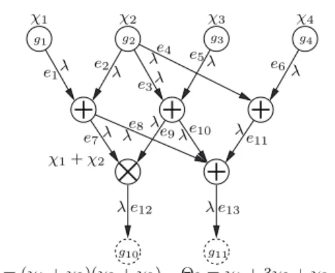
dis-tributed incoming data sources, where the data dependency can be represented by amultiple-input multiple-output di-rected acyclic graph (MIMO-DAG), as shown in the
illus-χ1+χ2 χ1 χ2 χ3 χ4 g11 g3 g4 e9 e10 e 11 e2 e6 e7 λ e1 λ λe8λ λ λ λ e4 e3λ λ e5λ λ e12 λe13 λ Θ1= (χ1+χ2)(χ2+χ3) Θ2=χ1+ 3χ2+χ3+χ4 g1 g10 g2
(a) An illustrative example of a cloud computing programming framework
n1 n2 n3 n4
n5 n6 n7 n8
n9 n10 n11 n12
n13 n14 n15 n16
(b) A 16-node 2-D torus interconnection topology.
Figure 1: An illustrative example of deploying a cloud computing programming framework over an underlying network infrastructure: (a) Computing functions Θ1 and Θ2 at computation rate λ; the data dependencies are represented by a MIMO-DAG structure; (b) An illustration of a 2-D torus in-terconnection topology commonly seen in large data centers or supercomputers.
trated example in Fig. 1(a).1 On the other hand, the under-lying networked system(upon which any cloud computing framework needs to be deployed) can also be represented by a graph. For example, Fig. 1(b) illustrates a 2-D torus inter-connection topology commonly found in large data centers or supercomputers that support cloud computing jobs. As will be shown later, to capture the key features of cloud com -puting programming frameworks and incorporate com puta-tion and communication constraints of the underlying net-works, we develop a genericmathematicalmodeling fram e-work, based on which we formulate the computation rate utility maximization problem (CRUM). Our main results and contributions in this paper are three-fold:
• By accounting for in-network data aggregation flows, we show that one can construct a new network flow model with ageneralized flow-conservation lawto address both 1The addition andmultiplication operations in Fig. 1(a) are only for illustrative purposes. Each vertex could be any general data processing operations.
communication limits and computation costs in Problem
CRUM. We point out that this utility framework and the associated generalized flow-conservation law are im por-tant in that they shares the same separable structure as in the classical network utilitymaximization problems in data communication networks [8, 9]. Thus, they enable the design of polynomial-time distributed algorithms for cloud computing by drawing experiences gained fromthe classical network utilitymaximization theory.
• By appropriately reformulating Problem CRUM in the Lagrangian dual domain, we reveal key separable proper-ties of the dual function of Problem CRUM. These key structural properties enable us to obtain closed-form ex-pressions for the primal and dual update schemes, which further leads to a fully distributed algorithmic implem en-tation for big data analytics in cloud computing.
• We offer important networking insights and economics in-terpretations for the proposed distributed algorithm. We also point out the connections to and distinctions from
the dual decomposition based distributed algorithms in the classical network utilitymaximization theory for data communications networks, thus further advancing our un-derstanding of distributed approaches in cloud computing network optimization theory. We also provide numerical examples to show the efficacy of our proposed distributed algorithm.
To our knowledge, this paper is among the first that treat the design of distributed algorithms in MIMO-DAG based cloud computing frameworks (e.g., Dryad) via a rigorous theoretical network-flow optimization approach. The
re-mainder of this paper is organized as follows. In Section 2, we review some related work in the literature, putting our work in a comparative perspective. Section 3 introduces the new network flowmodel with a generalized flow-conservation law for deploying cloud computing frameworks. Section 4 develops the principal components of our proposed distributed algorithm for solving Problem CRUM. Section 5 provides numerical results and Section 6 concludes this paper.
2.
RELATED WORK
Our work is closely related to i) distributed cross-layer utility maximization theory for data communication net-works (see, e.g., [10] for an overview) and ii) in-network computation techniques. In the in-network computation lit-erature, our work ismost related to [11], where Shahet al. developed a network flowmodel for the in-network com pu-tation in sensor network applications. The model in [11] extends the conventional flow-conservation law in the net-work flow literature [12] to in-netnet-work computation appli-cations. However, the model in [11] is restricted to simple tree topologies that are used for data aggregation in sen-sor networks. In contrast, our network flow model works with generic MIMO-DAG, which are themost appropriate
models for complex cloud computing programming fram e-works, such as Dryad and MapReduce. Also, in our network
model, we incorporate general network utility and comm u-nication/computation cost functions, which were not con-sidered in [11].
Our networkmodel also shares some similarities with the load shedding and distributed resource control problem of streamprocessing networks (e.g., [13–15]). But our work
differs fromthese works in the following two important as-pects: First, although the issue of flow imbalance in stream
processing networks was also pointed out in [14,15], the flow imbalance in [14,15] was caused by different flow production and consumption rates between upstreamand downstream
nodes. In contrast, the flow imbalance in this work is due to subcomputation in clouds, which is a fundamentally dif-ferent cause. Second, in [13], the task-to-server assignment relationship is assumed to be given and the authors only studied the end-to-end utility rate maximization. In con-trast, the task-to-sever assignment relationship is also part of the overall optimization in our work. Our network flow
model also has connections with the graph embedding prob-lems in graph theory (e.g., [16–18]). But these problems differ fromours in that their embedding objectives were to
minimize some graph-theoretic performancemetrics, such as dilation (i.e., themaximumdistance in the network between adjacent tree nodes).
3.
NETWORK MODEL AND PROBLEM
FOR-MULATION
In this section, we first present the modeling details of cloud computing programming frameworks and the under-lying network infrastructure in Section 3.1. Then, the con-cept of mapping between a programming framework and network infrastructure is introduced in Section 3.2. Next, we develop a new network flow model with a generalized flow-conservation law in Section 3.3. Finally, based on the network flowmodel, we formulate the computation rate op-timization problemin Section 3.4.
3.1
Modeling Cloud Co
m
puting Fra
m
eworks
and Network Infrastructure
As mentioned earlier, we model a cloud computing pro-gramming framework by a MIMO-DAG. Here, we denote a MIMO-DAG byD={V,E}, whereV and E represent the sets of vertices and edges, respectively, with|V| = V and
|E|=E. We note that this MIMO-DAG structure captures the parallel processing and multi-stage aggregation nature of typical cloud computing programming frameworks, such as Dryad ormultiple concatenations of Map/Reduce.
We suppose that there areS vertices of in-degree-zero in
D, corresponding to the S distributed input data sources. Without loss of generality (w.l.o.g), we label these source vertices asg1, . . . , gS. Formodeling convenience, there are K vertices inD having in-degree-one and out-degree-zero, corresponding to the virtual sinks that absorb the final out-put of Θk,k= 1, . . . , K. Again, w.l.o.g, we label such sinks
as gV−K+1, . . . , gV. The remaining nodes gS+1, . . . , gV−1 performthe computations prescribed by Θ. The input data stream at each sourcegi is denoted as {χi(k)}∞k=0, where χi(k) represents the i-th input element at time instant k.
The infinite input data streams could represent, for exam -ple, the “big data” phenomenon exemplified in the large data sets processing in by the MapReduce or Dryad frameworks in cloud computing. In this paper, all sources are assumed to be synchronized. We note that the synchronization in cloud computing systems is also an actively research topic (see, e.g., [19] and references therein) and its details are be-yond the scope of this paper. For simplicity, we assume that all input data streams and all directed edges in the MIMO-DAG structure have a homogeneous input rateλ, which can
also be thought of as the end-to-end computation rate of
{Θk}. We remark that the cases with heterogeneous rates
(due to compression or expansion processing) can be exer-cised similarly by introducing coefficients in front of the data rates [14] in our utilitymaximization formulation described later. One can further transformsuch cases into a hom oge-neous case usingmodeling techniques in [13] by changing the
measure and absorbing the coefficient into the resource us-age parameters. Hence, this homogeneous rate assumption does not lose any generality.
We leth(e) andt(e) denote the head and tail vertices of each directed edge e in E, respectively. We let S {e ∈ E|h(e) ∈ {g1, . . . , gS}} be the set of all edges originating
fromthe sources. We note that|S| ≥ S in general. Like-wise, we letK {e ∈ E|t(e) ∈ {gV−K+1, . . . , gV}}denote
the set of edges terminated at the sinks. Note that, since each sink edge represents a unique output (see Fig. 1(a)), we have |K| = K. W.l.o.g, we label the edges in E in such a way that the first|S|edges e1, . . . , e|S| and the last
K edgeseE−K+1, . . . , eE are the source and sink edges,
re-spectively. In Fig. 1(a), for example, S ={e1, . . . , e6} and
K={e12, e13}.
We point out that each directed edge inDcan be viewed as a subcomputation task. For example, in Fig. 1(a), edgee7
corresponds to the computation resultχ1+χ2. Therefore, the terms “edge” and “subcomputation” are sometimes used interchangeably in this paper. It should be noted, however, that a subcomputation does not necessarily correspond to a unique edge. For example, in Fig. 1(a), edgese7 ande8 all carry the same subcomputationχ1+χ2. The set of successor edges ofe in Dis defined as Ψ(e) {e ∈ E|t(e) =h(e)}. For example, in Fig. 1(a), the successor edges ofe2aree7and
e8. Note that fromthe structure ofD, we have Ψ(ei) =∅
for all ei ∈ K. Finally, we remark that the MIMO-DAG
structure degenerates into a tree topology if it has a single sink and each edge only has one successor edge. Therefore, the tree-structuremodel considered in [11] can be viewed as a special case of ourmodel.
On the other hand, in cloud computing environments (e.g., data centers or supercomputers), we have a networked sys-temas the physical computing and communication infras-tructure (i.e., a cloud computing hardware platform). Usu-ally, the hardware platform also exhibits certain carefully constructed parallel structures. For example, Fig. 1(b) il-lustrates a 2-D torus interconnection topology that is com
-monly seen in cloud hardware platforms. Advanced super-computers nowadays could employ torus interconnections with even higher dimensions (e.g., 5-D torus in IBM Bue Gene/Q architecture). But we point out that these special topology properties are not essential to our networkmodels and our distributed algorithmdesign, both of which apply to general interconnection topologies. In this paper, we also
model the underlying cloud computing hardware platform
by a graph G = {N,L}, where N and Lare the sets of nodes and links with |N | = N and |L| = L, respectively. Depending on the size and scale of the hardware system, each node in N could represent, e.g., a CPU core, a node card, or even a computer rack. Each link in Lrepresents the communication connection between the nodes. It could represent a local high-speed bus if the nodes are co-located on the same card or a fiber link if the nodes are located at different racks.
u-nications in cloud computingmodels (such as Map/Reduce and Dryad), it is highly desirable to allocate subcom puta-tion tasks involving input data sources and outputs at their physical locations. Therefore, w.l.o.g, we label the nodes of N as n1, . . . , nN in such a way that the first S nodes n1, . . . , nScorrespond to the physical locations of theSdata
sources ofD.
3.2
Mapping a Cloud Co
m
puting Fra
m
ework
onto a Network Infrastructure
Clearly, deploying a given cloud computing framework on a cloud computing hardware platformamounts tomapping all edgesinDontoGin an appropriate fashion. As in stan-dard graph theory terms, we define a pathP as a sequence of nodes inN such that every two adjacent nodesnkandnl
inP satisfy (nk, nl)∈ L. The first and the last nodes inP
are called the start and end nodes and are denoted asα(P) andβ(P), respectively. In the extreme case,P could contain only one node, saynk. In this case,α(P) =β(P) =nkand
the link (nk, nk) degenerates into a self-loop. Here, if an edge
is mapped to a path P, itmeans that the data are
trans-mitted fromα(P) via the specified links to β(P) and then the corresponding subcomputation is performed atβ(P). In the special case, if an edge ismapped to a self-loop, then the corresponding subcomputation task is performed locally and no communication is needed.
We denote the set of all paths inGasP. Avalid mapping ofDontoG is defined as follows:
Definition 1. A mapping M : E → P is valid if: (1)
α(M(ei)) = nk if ei ∈ S and h(ei) = gk, k = 1, . . . , S;
(2) β(M(ei)) =nk if ei ∈ Kandnk is the physical output
location ofei; and (3) α(M(ej)) =β(M(ei))if ej∈Ψ(ei).
In Definition 1, conditions (1) and (2) imply that the source and the sink nodes in D have to match to their physical locations in the underlying network, and condition (3) rep-resents that the logical successor relationships of the edges inDneed to be respected after themapping.
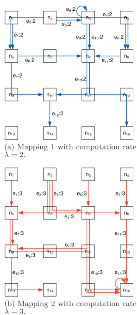
In general, there aremany different ways tomapDonto
G. For example, it is not difficult to see that Figs. 2(a) and 2(b) illustrate two validmappings of the MIMO-DAG structure in Fig. 1(a) onto the network in Fig. 1(b). Note that in a valid mapping, the node sequence corresponding to an edge in D could consist of multiple connected links inG. For example, in Figure 2(b), edgee8 consists of links (n5, n9), (n9, n10), and (n10, n11).
We note that eachmappingmay use a different com puta-tion rate, as shown in Figs. 2(a) and 2(b). For example, in Fig. 2(a), the label “ei: 2” represents that the computation
rate of each edgeei is 2 in thismapping. Further, a tim
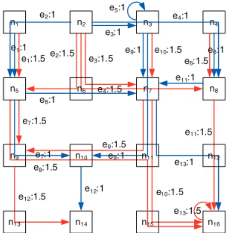
e-sharing among validmappings also yields a validmapping. For instance, Fig. 3 shows a time-sharing between the two
mappings in Figs. 2(a) and 2(b), each accounting for 50% of time. It is not difficult to see that the computation rate of this time-sharingmapping is 0.5×2 + 0.5×3 = 2.5.
3.3
A Network Flow Model with a Generalized
Flow-Conservation Law
It can be seen fromthe above discussions that the com-putation rate regionof a cloud computing framework over a given network infrastructure can be exhausted by all tim e-sharing strategies among all possible valid mappings. As a result, any performance metrics related to the com
pu-e1:2 e2:2 e5:2 e6:2 e3:2 e4:2 e7:2 e8:2 e9:2 e10:2 e11:2 e12:2 e13:2 n2 n5 n8 n9 n10 n12 n13 n14 n15 n16 n1 n6 n7 n11 n3 n4
(a) Mapping 1 with computation rate
λ= 2. e1:3 e2:3 e3:3 e4:3 e5:3 e6:3 e7:3 e9:3 e8:3 e10:3 e11:3 e12:3 n1 n2 n3 n4 n5 n6 n7 n8 n9 n10 n12 n14 n15 n16 e13:3 n11 n13
(b) Mapping 2 with computation rate
λ= 3.
Figure 2: Two valid mappings of the MIMO-DAG
structure in Fig. 1(a) onto the network in Fig. 1(b). Eachmapping has a different computation rate.
tation rate can be optimized by determining an optimal time-sharing strategy. However, since the total number of validmappings is exponential inN, finding an optimal tim e-sharing strategy directly is intractable. Therefore, we need to exploit additional structure of the networked system to address this challenge.
To this end, our basic idea is to develop a new network flow modelwith ageneralized flow-conservation lawfor com -putation analytics. The fundamental rationale behind this approach is that, similar to the classicalmodel in them ulti-commodity network flow literature [12], the structural prop-erties of the new network flow model would also lead to polynomial time solutions if designed appropriately.
Unfortunately, developing a flow-conserved network flow
model for computation analytics is not-trivial. Due to per-forming computations at each node in the network, the clas-sical flow-conservation law [12] fails to hold in computation analytics network flows. For example, fromthe zoom-in view for noden10in Fig. 4, it can be seen that the total incoming flow rate is:
x(e7) (n9,n10)+x( e8) (n9,n10)+x( e9) (n10,n11)+x( e9) (n10,n11)= 5.
n1 n2 n3 n4 n5 n6 n7 n8 n9 n10 n14 n15 n16 n13 n12 e2:1 e1:1 e1:1.5 e8:1.5 e7:1.5 e7:1 e3:1 e5:1 e2:1.5 e3:1.5 e4:1.5 e4:1 e12:1.5 e12:1 e9:1.5 n11 e13:1 e9:1 e9:1 e10:1.5 e11:1 e6:1.5 e6:1 e8:1 e11:1.5 e10:1.5 e13:1.5
Figure 3: A time-sharing between twomappings in Fig. 2(a) and Fig. 2(b), each accounting for 50% of time. e8:1.5 e9:1.5 e12:1 e7:1 e8:1.5 link (n10,n9) link (n11,n10)
n
10 link (n10,n14) e9:1 e9:1.5 link (n9,n10) link (n10,n11)Figure 4: Zoom-in view of noden10in Fig. 3. Due to the addition computations, the total incoming and outgoing flow rates atn10 are not equal.
noden10, the total outgoing flow rate is:
x((en9) 10,n9)+x (e8) (n10,n11)+x (e12) (n10,n14)= 4.
This shows that, for computation analytics in cloud com put-ing, the total input and output network flow are unbalanced. Although the traditional flow-conservation law no longer holds here, upon a closer look at each incoming edge and their corresponding outgoing or successor edges atn7, it is not difficult to observe another form of flow-conservation law. As shown in Fig. 4, for the incoming edgee4that does not involve any computation atn7, we have:
x((en9)
11,n10)=x( e9)
(n10,n9),
i.e., the incoming rate equals the outgoing rate. The same is also true for the incoming edge e8. On the other hand, for the incoming edgee7 that involves in the addition with incoming edgee9, we have:
x(e7) (n9,n10)=x( e12) (n10,n14) and x( e9) (n11,n10)=x( e12) (n10,n14),
i.e., the outgoing rate of the successor edge ofe7is equal to the incoming rate ofe7.
Tomodel this new formof flow-conservation law, it is im -portant to recognize that: for a subcomputation, saye, that is injecting to noden, a portion of its flow is terminated atn
to compute the successor edges ofe(i.e., Ψ(e)). For conve-nience, we label the links in the physical network as 1, . . . , L
instead of using node pairs (nj, nk). We letx(le) ≥0
repre-sent the flow amount of subcomputation taskeon linkl. In all validmappingsM, since the start node of a source edge
ei∈ S and the end node of a sink edgeei ∈ K are always
mapped to their respective physical nodes in the network, we let Src(ei)α(M(ei)) and Dst(ei)β(M(ei)) be the
physical source and end nodes of ei and ei for simplicity.
Then, based on the previous observations, we have the fol-lowing result:
Lemma 1. When computation analytics are performed over an underlying networked system, the following generalized flow-conservation law holds:
l∈O(nk) x(ei) l +y (ej) nk − l∈I(nk) x(ei) l −y (ei) nk =λ, ∀ei∈ S, ∀ej∈Ψ(ei), nk= Src(ei), (1) l∈O(nk) x(lei)+y(nekj)− l∈I(nk) x(lei)−y(ei) nk = 0, ∀ei∈ E\K, ∀ej∈Ψ(ei), andnk= Src(ei) ifei∈ S, (2) l∈O(nk) x(lei)− l∈I(nk) x(lei)−y(ei) nk = 0, ∀ei∈ K, nk= Dst(ei), (3) l∈O(nk) x(ei) l − l∈I(nk) x(ei) l −y( ei) nk =−λ, ∀ei∈ K,nk= Dst(ei), (4)
where O(nk) andI(nk) represent the sets of outgoing and
incoming links at nodenk, respectively; andy( ei)
nk represents
the subcomputation ei generated at nodenk.
Here, the equalities in (1) and (2) represent that the total incoming flow rate of any non-sink edgeeiat nodenkshould
be equal to the sum of the outgoing flow rates of ei and
its successor edgeej, and this relationship holds for every
successor edge of ei. Moreover, Eq.(1) states that if ei is
a source edge andnk happens to be its source node, then
the net injection rate of ei atnk isλ. On the other hand,
Eqs.(3) and (4) say that, for a sink edge ei that does not
have any successor edge, the net output flow rate should be equal toλat its physical location and zero elsewhere.
3.4
Proble
m
For
m
ulation
We letCldenote the capacity of linkl. Since the total
net-work flow traversing a link cannot exceed the link’s capacity, we haveEi=1x(ei)
l ≤Cl,l= 1, . . . , L. We let the network
utility be a function ofλ, denoted by U(λ) :R+ →R. We assume thatU(λ) is concave,monotonically increasing, and twice continuously differentiable. The concavity ofU(·) rep-resents the “diminishing returns” effect. WhenU(·) is linear (as a special case of concavity), we are simplymaximizing the computation rate itself.
In the physical network, each outgoing edge at a node represents a subcomputation (see, e.g., edgese9,e10, ande13
in Fig. 4), which incurs certain costs (e.g., consumed energy per unit amount of computation). We letρk represent the
unit cost for performing computation at nodenk. Then, the
as: |S| i=1 ρk ⎛ ⎝λ+y(ei) nk + l∈I(nk) x(ei) l − l∈O(nk) x(ei) l ⎞ ⎠+ E−K i=|S|+1 ρk ⎛ ⎝y(ei) nk + l∈I(nk) x(lei)− l∈O(nk) x(lei) ⎞ ⎠. (5) In (5), the termλ+y(ei) nk + l∈I(nk)x( ei) l − l∈O(nk)x( ei) l
is the total flow rate of source edgeei that is terminated
at nodenk and used to compute its successor edges.
Like-wise, the termy(neki)+ l∈I(nk)x (ei) l − l∈O(nk)x (ei) l
rep-resents the total flow rate of non-source and non-sink edge
ei terminated atnk. Our objective is tomaximize the net
network utility, defined as network utilityminus the total costs. Putting together the discussions earlier, we can
for-mulate the problemas follows:
CRUM: MaxU(λ)− N k=1 ⎛ ⎝|S| i=1 ρk ⎛ ⎝λ+y(neki)+ l∈I(nk) x(lei) − l∈O(nk) x(lei) ⎞ ⎠+ E−K i=|S|+1 ρk ⎛ ⎝y(ei) nk + l∈I(nk) x(lei)− l∈O(nk) x(lei) ⎞ ⎠ ⎞ ⎠ s.t. Eqs. (1), (2), (3), (4), E i=1 x(lei)≤Cl, ∀l= 1, . . . , L, x(ei) l ≥0, ∀i, l; λ≥0.
Now, it is not difficult to recognize that with the pro-posed network flowmodel in Lemma 1, ProblemCRUM is a convex program. Moreover, the nice separable structure of the objective function enables the design of distributed algorithmto solve ProblemCRUM, which will be the focus of the next section.
4.
DISTRIBUTED SOLUTION PROCEDURE
In this section, we will present the key steps in design-ing a distributed algorithmbased on dual decomposition to solve ProblemCRUM. In Section 4.1, we will first reform u-late ProblemCRUM into its Lagrangian dual problemand show how to appropriately decompose the Lagrangian dual problem. Based on these results, we introduce the basic idea in designing a distributed algorithmin Section 4.2. In Sec-tion 4.3, we offer some interesting networking and economics interpretations of the proposed distributed algorithm. Then, we will present some numerical results in Section 5.
4.1
Lagrangian Dual Refor
m
ulation and
De-co
m
position
As mentioned earlier, since Problem CRUM is a convex program, it can be equivalently solved in its Lagrangian dual domain because of a zero duality gap [20]. To solve the Prob-lemCRUM in its Lagrangian dual domain, we first slightly
modify the constraints in (1)–(4) into inequality constraints as follows: l∈O(nk) x(ei) l +y (ej) nk − l∈I(nk) x(ei) l −y (ei) nk ≥λ, ∀ei∈ S, ∀ej∈Ψ(ei),nk= Src(ei), (6) l∈O(nk) x(lei)+yn(ekj)− l∈I(nk) x(lei)−y(ei) nk ≥0, ∀ei∈ E\K, ∀ej∈Ψ(ei), andnk= Src(ei) ifei∈ S, (7) l∈O(nk) x(lei)− l∈I(nk) x(lei)−y(ei) nk ≥0, ∀ei∈ K,nk= Dst(ei), (8) l∈O(nk) x(ei) l − l∈I(nk) x(ei) l −y( ei) nk ≥ −λ, ∀ei∈ K,nk= Dst(ei), (9)
It is not difficult to show that thesemodifications do not affect the solution at optimality. Interestingly, these m od-ifications can also be interpreted from a network stability perspective: the total service rate at each node is no less than the total arrival rate.
Next, we associate dual variablesμ(kij) ≥0 and w(ki) ≥0 for each constraint in (6)–(7) and (8)–(9), respectively. For notational simplicity, we use Ψi to represent the index set {j : ej ∈ Ψ(ei)}. Also, we use vectors x, μ, and w to
group all x-, μ- and w-variables. By accommodating the constraints into the objective function and combining re-lated terms, we have that the Lagrangian can be written as follows: L(λ,x,μ,w) =U(λ)− N k=1 ⎛ ⎝|S| i=1 ρk ⎛ ⎝λ+y(neki)+ l∈I(nk) x(lei)− l∈O(nk) x(lei) ⎞ ⎠+ E−K i=|S|+1 ρk ⎛ ⎝y(ei) nk + l∈I(nk) x(lei)− l∈O(nk) x(lei) ⎞ ⎠ ⎞ ⎠ + E i=1 j∈Ψi N k=1 μ(kij) ⎛ ⎝ l∈O(nk) x(ei) l +y (ej) nk − l∈I(nk) x(ei) l −y (ei) nk ⎞ ⎠ + E i=E−K−1 N k=1 w(ki) ⎛ ⎝ l∈O(nk) x(lei)− l∈I(nk) x(lei)−y(ei) nk ⎞ ⎠ + (−λ) |S| i=1 j∈Ψi μ(Src(ij)i)+λ E i=E−K+1 w(Dst(i) i). (10)
Then, the Lagrangian dual function can be written as: Φ(μ,w) = sup λ,x L(λ,x,μ,w) E i=1x( ei) l ≤Cl,∀l, x(ei) l ≥0,∀i, l;λ≥0. ) .(11) Finally, the dual problemcan be written as:
D: Minimize Φ(u)
subject to u≥0. (12)
Next, it is important to recognize that the Lagrangian function in (11) possesses a decomposable structure, which leads to a distributed computation scheme. More specifi-cally, by appropriately switching summation orders and re-arranging terms in (11), we have the following result (see Appendix A for proof details):
Proposition 2. The Lagrangian in (11) can be decom-posed in a source-wise and link-wise fashion as follows:
Φ(μ,w) = ΦFC(μ,w) + L l=1 Φ(Rl)(μ,w) + N k=1 Φ(Ck)(μ,w),
whereΦFC(μ,w),Φ(Rl)(μ,w), andΦ(Cn)(μ,w) represent the flow control, per-link routing, and per-node computation sub-problems at each source, each link, and each node, respec-tively. Here,ΦFC(μ,w) and ΦR(l)(μ,w) are defined as fol-lows, respectively: ΦFC(μ,w)max λ≥0 U(λ)− λ |S| i=1 j∈Ψi μ(Src(ij)i)+ N k=1 ρk − E i=E−K+1 wDst((i) i) ) ; Φ(Rl)(μ,w) max E i=1 ˜ w(Tx(i) l)−w˜Rx((i)l) x(ei) l s.t. E i=1 x(lei)≤Cl, x( ei) l ≥0,∀i. ) ,
wherew˜(ki),∀k= 1, . . . , N, ∀i= 1, . . . , E, are defined as: ˜ wk(i) ρk+ j∈Ψiμ(kij), i= 1, . . . , E−K, wk(i)+j∈Ψiμk(ij), i=E−K+ 1, . . . , E; (13) Φ(Ck)(μ,w)max y(nkei)≥0,∀i E i=1 j∈Ψi μ(kij)(y(nekj)−y(neki))−wˆ( i) k y (ei) nk ) ,
wherewˆ(ki),∀k= 1, . . . , N, ∀i= 1, . . . , E, are defined as: ˜
wk(i)
ρk, i= 1, . . . , E−K,
wk(i), i=E−K+ 1, . . . , E. (14)
Based on Proposition 2, the Lagrangian dual problem D in (12) can be transformed into the following master dual problem: MD:Minimize ΦF C(μ,w) + L l=1 Φ(Rl)(μ,w) + N k=1 Φ(Ck)(μ,w) subject toμ≥0, w≥0.
Then, the task of solving the Lagrangian dual problem D boils down to distributedly solving the subproblems ΦF C(μ,w),
ΦR(l)(μ,w), and ΦC(k)(μ,w), and then themaster dual prob-lemMD.
4.2
Design of Distributed Algorith
m
Note that at each source node, the flow control and com -putation subproblems ΦF C has a concave objective
func-tion with a single non-negative decision variable. Thus, ΦF C can be trivially and efficiently solved (e.g., by sim
-ple bisection searchmethod). Also, it can be observed that the routing subproblemΦ(Rl) at each link is a lower dim en-sional linear programming problem(with a single constraint,
O(EV2) variables, and all problem coefficients are locally available), whichmeans that it can be efficiently solved as
Algorithm1A subgradient algorithmfor solving Problem
CRUM.
Initialization:
1. Choose initial starting pointsμ(0)andw(0). Letm= 0.
Main Iteration:
2. Compute the source computation rateλ(m) by solving the flow control subproblemΦF C(μ(m),w(m)) by using,
e.g., bisectionmethod.
3. Compute the routing decisionsx(ei)
l (m) at each link by
solving the routing subproblemΦR(μ(m),w(m)), a linear
programming problem.
4. Choose an appropriate step sizeπm. Compute the
sub-gradientsd(μ,kij)(m) andd(w,ki) (m) using (17) and (18) with
λ(m) andx(lei)(m).
5. Update dual variablesμ(m+1)andw(m+1)withd(μ,kij)(m) andd(w,ki) (m).
6. Ifμ(m+1)−μ(m)< andw(m+1)−w(m)< , then
returnλ(m) andx(ei)
l (m). Otherwise, letk←k+ 1 and
go to Step 2.
well. For the master dual problemMD, since its objective function is piece-wise differentiable, one can apply subgra-dientmethod [20]. More specifically, starting with an initial
μ(0) and w(0) and after evaluating Φ
F C(μ(m),w(m)) and
Φ(Rl)(μ(m),w(m)) in them-th iteration, we update the dual
variables as follows:
μ(kij)(m+ 1) =max{μ(kij)(m)−πmdμ,k(ij)(m),0}, (15)
w(ki)(m+ 1) =max{wk(i)(m)−πmd(w,ki) (m),0}, (16) whereπm>0 denotes a positive scalar step size, andd(ij)
μ,k(m)
andd(w,kij)(m) represent the subgradients of the dual variables
μ(kij) andwk(i) in them-th iteration, respectively.
It is known that for the subgradient iterative schemes in (15) and (16) to converge, a sufficient condition is that the step size πm satisfies πm → 0 as m → ∞, ∞m=0 = ∞, and∞m=0(πm)2[20]. A popular step size selection strategy is the divergent harmonic series: πm = β
m, m = 1,2, . . .,
where β is some given systemparameter. For the master dual problemMD, the subgradient for the Lagrangian dual function in (10) can be computed as:
d(μ,kij)(m) = l∈O(nk) x(ei) l +y (ej) nk − l∈I(nk) x(ei) l −y(ei) nk −λ{ei∈S,nk=Src(ei)}, (17) d(w,ki) (m) = l∈O(nk) x(lei)− l∈I(nk) x(lei) −y(ei) nk +λ{ei∈S,nk=Dst(ei)}, (18)
where {·} represents the indicator function, which equals 1 if the condition in {·} is satisfied and 0 otherwise. To summarize, the design of distributed subgradient algorithm
for solving ProblemCRUM is illustrated in Algorithm1.
4.3
Networking and Econo
m
ics Interpretations
Several interesting networking and economics insights for the subgradient-based distributed algorithmare in order.
It can be seen that by dividing the step size πm on both
sides of (15) and (16) and lettingQ(kij)(m)μ(kij)/πmand ¯ Q(ki)(m)w(ki)/πm, we have: Q(kij)(m+ 1) =max Q(kij)(m)− l∈O(nk) x(ei) l −y (ej) nk +yn(eki) + l∈I(nk) x(ei) l +λ{ei∈S,nk=Src(ei)},0 ) , (19) ¯ Q(ki)(m+ 1) =max ¯ Q(ki)(m)− l∈O(nk) x(lei) −λ{ei∈S,nk=Dst(ei)}+ l∈I(nk) x(ei) l +y (ei) nk ,0 ) . (20)
A closer look reveals that (19) and (20) behave exactly the same as “queue length evolution” as seen in traditional data communications networks. Indeed, if we letQ(kij)(m) repre-sent the queuing backlog for computing the successive edge
j of edge i at node k in time instant m, then this queu-ing backlog and the dual variable μ(kij)(m) are intimately related (differ only by a scaling factor πm). By the same
token, ¯Q(ki)(m) can be similarly interpreted as the queuing backlog of the terminating edgesei∈ Kat nodem.
Connections to the back-pressure algorithm: Clearly, in cases where in-network computation is disabled, i.e., by forcingx(lej)= 0 for allej∈Ψ(ei) and for alll, the network
degenerates into a traditional communication network. As expected, it is easy to check that the queue length evolutions in (19) and (20) reduce to the conventional queue length evolution: Q(ki)(m+ 1) =max Q(ki)(m)− l∈O(nk) x(ei) l + l∈I(nk) x(ei) l +λ {ei∈S,nk=Src(ei)}−{ei∈S,nk=Dst(ei)} ,0 ) . (21) Moreover, since all dual μ-variables become 0, it is easy to verify that the computation subproblem Φ(Ck) admits a trivial optimal solution: y(neki) = 0, ∀k, i. Also, with dual μ-variables being 0, it is not difficult to see that the routing subproblemΦ(Rl)(w) admits a trivial solution as follows: for a given linkl, pick a subcomputation taskei that has the
largest ( ˜wTx((i)l)−w˜Rx((i) l))-value, saye∗i, and lete∗i use up the
link capacity Cl. This is exactly the same strategy used
in the celebrated “back-pressure” algorithmthat was first discovered in [21].
Pricing interpretation of the dual subgradient up-dating scheme: The dual variablesμ(kij)(m) andw(ki)(m) can also be economically interpreted as “congestion prices” at nodekduring them-iteration. The dual updating scheme of the subgradient algorithmcan then be viewed as a pricing scheme. When nodekbecomes increasingly congested, then
d(μ,kij) < 0. From (15), we can see the price of nodek will be increased. On the other hand, when nodekbecomes less congested, thend(μ,kij) >0. Again, from(16), it can be sen that the price will be decreased.
0 1 2 3 4 5 6 7 8 9 10 11 12 13 14 15 16 0 5 10 15 20 25 30 NodeID Flo w R ate NorthOut SouthOut EastOut WestOut Self Comp.
Figure 5: Outgoing links and self-loop flow rates at each node for edgee12.
0 1 2 3 4 5 6 7 8 9 10 11 12 13 14 15 16 0 5 10 15 20 25 30 NodeID Flo w R ate NorthOut SouthOut EastOut WestOut Self Comp.
Figure 6: Outgoing links and self-loop flow rates at each node for edgee13.
5.
NUMERICAL RESULTS
In this section, we use Fig. 1 as an example to illustrate our proposed network flow model and distributed solution procedure. That is, we want to optimize the deployment of the MIMO-DAG computation framework in Fig. 1(a) onto the 16-node 2-D torus interconneced network in Fig. 1(b). The physical locations of both Θ1 and Θ2 are at noden16. Here, we let the capacity of each link in Fig. 1(b) be 10 and let the per-node unit computation cost be 0.001. Our objective is to maximize the computation rate, i.e., letting
U(λ) =λ. After optimization, the maximumcomputation rate is 15.95. Due to space limitation and the large number of optimal link flow rate variables for this example (5×16× 13 = 1040 variables), we only plot in Figs. 5 and 6 the outgoing links and self-loops flow rates for edgese12ande13
to illustrate part of the optimal solution. The “North Out,” “South Out,” “East Out,” and “West Out” in Figs. 5 and 6 represent the outgoing links at each node in Fig. 1(b) along the specified directions, respectively. Recall fromFig. 1(a) that edges e12 and e13 are sink edges, which correspond to the final results of functions Θ1 and Θ2, respectively. Surprisingly, it can be seen that the computations of these sink edges are not deployed close to the physical output node
n16. Themajority of the computations ofe12 and e13 are done at node 2 (see the rates of self-loops at node 2 and node 1). This shows that the heuristic “proximity” deployment rulemay not be optimal. FromFigs. 5 and 6, it is also not difficult to see the optimal routing paths for edgese12 and
1 2 3 4 5 6 7 8 9 10 0 2 4 6 8 10 12 14 16 18
Normalized Nodal Computation Cost
N ormali z ed C om p uation R ate
Figure 7: The change ofmaximumend-to-end com -putation rate with respect to the change of per-node unit computation cost.
10 20 30 40 50 60 70 80 90 100 0 20 40 60 80 100 120 140 160 180
NormalizedLink Capacity
N ormali z ed C om p uation R ate
Figure 8: The change ofmaximumend-to-end com -putation rate with respect to the change of link ca-pacity.
e13. For example, the optimal routing paths for edge e13
are:
n1→W n4→N n16, n2→E n3→E n4→N n16, n2→S n6→E n7→E n8→S n12→S n16, n2→W n1→W n4→N n16, n2→N n14→E n15→E n16, n12→S n16,
where the letter above each arrow denotes the routing di-rection at that hop. Next, we illustrate in Figs. 7 and 8 the changes ofmaximumend-to-end computation rate with re-spect to the changes of per-node unit computation cost and link capacity, respectively. In Fig. 7, we can see as expected that the end-to-end computation rate decreases as the unit computation cost at each node increases from1 to 10 units (step size is 0.001). Likewise, we can see from Fig. 8 the end-to-end computation rate increases as the link capacity increases from10 to 100.
6.
CONCLUSION
In this paper, we investigated the design of distributed algorithms for cloud computing programming frameworks deployments. We formulated the computation rate utility
maximization problem(CRUM) by developing a new net-work flow model with a generalized flow-conservation law. Based on this enabling framework, we developed a dual de-composition based distributed algorithmto solve Problem
CRUM. We provided important networking interpretations
and key implementation insights for our proposed algorithm
and pointed out the connections and distinctions to dis-tributed algorithms design in traditional data comm unica-tions networks. Collectively, these results serve as the first building block of a new theoretical framework for the de-ployment of cloud computing programming frameworks.
7.
REFERENCES
[1] A. S. Szalay, “Extreme data-intensive scientific computing,”IEEE Computing in Science and Engineering, vol. 13, no. 6, pp. 34–41, Nov. 2011. [2] “Data, data everywhere,” Economist, 2010. [Online].
Available: http://www.economist.com
[3] J. Dean and S. Ghemawat, “MapReduce: Simplified data processing on large clusters,” in Proc. USENIX OSDI, San Francisco, CA, Dec. 6-8, 2004, pp. 137–149. [4] M. Isard, M. Budiu, Y. Yu, A. Birrell, and D. Fetterly,
“Dryad: Distributed data-parallel programs from
sequential building blocks,” in Proc. ACM
SIGOPS/Eurosys, Lisboa, Portugal, Mar. 21-23, 2007, pp. 59–72.
[5] K.-H. Lee, Y.-J. Lee, H. Choi, Y. D. Chung, and B. Moon, “Parallel data processing with MapReduce: A survey,” ACM SIGMOD Record, vol. 40, no. 4, pp. 11–20, Dec. 2011.
[6] Y. Huai, R. Lee, S. Zhang, C. H. Xia, and X. Zhang, “DOT: Amatrixmodel for analyzing, optimizing and deploying software for big data analytics in
distributed systems,” inProc. ACM SOCC, Cascais, Portugal, Oct. 27-28, 2011.
[7] Hadoop.http://hadoop.apache.org.
[8] M. Chiang, S. H. Low, A. R. Calderbank, and J. C. Doyle, “Layering as optimization decomposition: A
mathematical theory of network architecture,”Proc. IEEE, vol. 95, no. 1, pp. 255–312, Jan. 2007. [9] F. P. Kelly, A. K. Malullo, and D. K. H. Tan, “Rate
control in communications networks: Shadow prices, proportional fairness and stability,”Journal of the Operational Research Society, vol. 49, pp. 237–252, 1998.
[10] X. Lin, N. B. Shroff, and R. Srikant, “A tutorial on cross-layer optimization in wireless networks,”IEEE J. Sel. Areas Commun., vol. 24, no. 8, pp. 1452–1463, Aug. 2006.
[11] V. Shah, B. K. Dey, and D. Manjunath, “Network flows for functions,” inProc. IEEE International Symposium on Information Theory (ISIT), St. Petersburg, Russia, Jul.31–Aug.5, 2011, pp. 234–238. [12] M. S. Bazaraa, J. J. Jarvis, and H. D. Sherali,Linear
Programming and Network Flows, 4th ed. New York: John Wiley & Sons Inc., 2010.
[13] H. Feng, Z. Liu, C. Xia, and L. Zhang, “Load shedding and distributed resource control of stream
processing networks,”Performance Evaluation, vol. 64, no. 9-12, pp. 1102–1120, Oct. 2007.
[14] H. Zhao, C. H. Xia, Z. Liu, and D. Towsley, “A unified
modeling framework for distributed resource allocation of general fork and join processing networks,” inProc. ACM Sigmetrics, New York, NY, Jun. 14-18, 2010. [15] Z. Liu, A. Tang, C. H. Xia, and L. Zhang, “A
networks,”Annals of Operations Research, vol. 170, no. 1, pp. 161–182, Sep. 2009.
[16] F. T. Leighton, M. J. Newman, A. G. Ranade, and E. J. Schwabe, “Dynamic tree embeddings in butterflies and hypercubes,”SIAM Journal of Computing, vol. 21, no. 4, pp. 639–654, Aug. 1992. [17] O. Wohlmuth and F. Mayer-Lindenberg, “Amethod
for the embedding of arbitrary trees into hypercubes,” inProc. ACM Symposium on Applied Computing, 1998, pp. 569–574.
[18] V. Heun and E. W. Mayr, “Efficient dynamic
embeddings of arbitrary binary trees into hypercubes,” Journal of Algorithms, vol. 43, pp. 51–84, 2002. [19] A. W. Malik, A. Park, and R. M. Fujimoto,
“Optimistic synchronization of parallel simulations in cloud computing environements,” inProc. IEEE International Conference on Cloud Computing, Bangalore, India, Sep. 21-25, 2009, pp. 49–56. [20] M. S. Bazaraa, H. D. Sherali, and C. M. Shetty,
Nonlinear Programming: Theory and Algorithms, 3rd ed. New York, NY: John Wiley & Sons Inc., 2006.
[21] L. Tassiulas and A. Ephremides, “Stability properties of constrained queuing systems and scheduling policies formaximumthroughput inmultihop radio
networks,”IEEE Trans. Autom. Control, vol. 37, no. 12, pp. 1936–1948, Dec. 1992.
APPENDIX
A.
PROOF OF PROPOSITION 2
To derive the subproblemΦFC(μ,w), we combine all terms in (10) related toλ, which leads to:
U(λ)−λ |S| i=1 j∈Ψi μ(Src(ij)i)+ N k=1 ρk − E i=E−K+1 wDst((i) i) .
Note that the above expression is exactly the objective func-tion of ΦF C in Proposition 2.
Next, we derive the objective function of Φ(Rl), which is relativelymore involved. First, it is not difficult to verify that by switching the summation order fromnode-based to link-based, we can rewrite the fouth termin (10) as:
E i=E−K−1 N k=1 w(ki) ⎛ ⎝ l∈O(nk) x(ei) l − l∈I(nk) x(ei) l −y (ei) nk ⎞ ⎠ = L l=1 E i=E−K+1 wTx((i)l)−w(Rx(i) l) x(ei) l − N k=1 E i=E−K+1 w(ki)y(ei) nk . (22) By the same token, we can immediately rewrite the partial second term(excluding the summation involvingλ) in (10) as: E−K i=1 N k=1 ρk ⎛ ⎝ l∈O(nk) x(lei)− l∈I(nk) x(lei) ⎞ ⎠−N k=1 E−K i=|S|+1 ρkyn(eki) = L l=1 E−K i=1 ρTx(l)−ρRx(l) x(ei) l − N k=1 E−K i=|S|+1 ρky(neki). (23)
Now, for themore complex third termin (10), we have
E i=1 j∈Ψi N k=1 μ(kij) ⎛ ⎝ l∈O(nk) x(ei) l +y (ej) nk − l∈I(nk) x(ei) l −y (ei) nk ⎞ ⎠ (a) = E i=1 N k=1 l∈O(nk) x(lei)− l∈I(nk) x(lei)−y(ei) nk j∈Ψi μ(kij) + j∈Ψi μ(kij)yn(ekj) = E i=1 N k=1 l∈O(nk) x(ei) l − l∈I(nk) x(ei) l j∈Ψi μ(kij) + E i=1 N k=1 j∈Ψi μ(kij) y(nekj)−y(neki) (b) = L l=1 E i=1 j∈Ψi μ(Tx(ij)l)− j∈Ψi μ(Rx(ij)l) x(ei) l + N k=1 E i=1 j∈Ψi μ(kij) x(lej)−y(ei) nk , (24)
where (a) holds because the summations of thex(ei)
l -variables
do not involve indexjand can be taken outside of the sum
-mation with respect to index j; and (b) follows from the same token as in (22) and (23) and the fact that switching the summation orders of thex(lej)-variables does not change their sumvalue.
Next, by adding (22), (23), (24) together and defining new ˜w- and ˆw-variables as in (13) and (14), we arrive at a summation of the following two terms:
L l=1 E i=1 ˜ w(Tx(i)l)−w˜Rx((i)l) x(ei) l ) , (25) N k=1 E i=1 j∈Ψi μ(kij)(y(nekj)−yn(eki))−wˆ( i) k y (ei) nk , (26)
which is exactly the objective function of Φ(Rl)and Φ(Ck). Note that the outer summation in (25) is with respect to link in-dices, each summand can be decomposed and computed at each link locally. Likewise, the outer summation in (26) is with respect to node indices, each summand can be decom -posed and computed at each node locally.
Finally, noting that the constraints Ei=1x(lei), ∀l, can also be separated in a link-wise fashion, we then have that themaximization ofL(λ,x,μ,w) can be equivalently com -puted as the sumof a series ofmaximization subproblems at the source and each link, which are defined as in Propo-sition 2. This completes the proof.