1616 P St. NW
Washington, DC 20036
S e p t e m b e r 2 0 0 8 R F F D P 0 8 - 2 8
The Incidence of
U.S. Climate Policy
Where You Stand Depends on Where
You Sit
D a l l a s B u r t r a w , R i c h S w e e n e y , a n d M a r g a r e t W a l l s
© 2008 Resources for the Future. All rights reserved. No portion of this paper may be reproduced without permission of the authors.
Discussion papers are research materials circulated by their authors for purposes of information and discussion. They have not necessarily undergone formal peer review.
The Incidence of U.S. Climate Policy:
Where You Stand Depends on Where You Sit
Dallas Burtraw, Rich Sweeney, and Margaret Walls
Abstract
Federal policies aimed to slow global warming would impose potentially significant costs on households that vary depending on the policy approach that is used. This paper evaluates the effects of a carbon dioxide cap-and-trade program on households in each of 11 regions of the country and sorted into annual income deciles. We find tremendous variation in the incidence (the distribution of cost) of the policy. The most important feature that affects households is how the policy distributes the value created by placing a price on CO2 emissions. We evaluate 10 policy alternatives that yield results that range from
moderately progressive (expansion of the Earned Income Tax Credit, investments in efficiency and cap-and-dividend) to severely regressive (reduce income taxes, free distribution to incumbent emitters and reduction of the payroll tax). To varying degrees the allocation of the value of emissions allowances amplifies or potentially resolves the tradeoff between equity and efficiency.
Key Words: cap-and-trade, allocation, distributional effects, cost burden, equity
Contents
Executive Summary ... i
1 Introduction... 1
2 Defining and Measuring Regressivity ... 4
3 The Literature on Distributional Impacts of Climate Policies ... 6
4 Data and Methodology... 9
4.1 Estimating the CO2 Content of Direct Energy Expenditures ... 9
4.2 Estimating the Indirect CO2 Content of Other Expenditures... 17
5 Effects of Pricing CO2... 21
5.1 How to Interpret Incidence and Alternative Policy Remedies... 24
6 Results for Alternative Policy Scenarios ... 27
6.1 Cap-and-Dividend (Lump Sum Transfers) ... 27
6.2 Reducing Preexisting Taxes... 31
6.3 Energy and Fuel Sector Adjustments... 37
6.4 Free Allocation to Emitters... 47
7 Discussion and Concluding Remarks ... 49
7.1 Observations and Major Trade-Offs ... 49
7.2 Options for Policymakers ... 57
7.3 Limitations and Research Needs... 57
References... 59
Appendix A... 63
Appendix B ... 64
Appendix C ... 65
The Incidence of U.S. Climate Policy:
Where You Stand Depends on Where You Sit
Dallas Burtraw, Rich Sweeney, and Margaret Walls Executive Summary
Federal climate policy would impose potentially significant costs on households, costs that would vary depending on the policy enacted. Cap and trade remains a leading candidate for climate policy because it is expected to be effective in identifying low-cost emissions reductions, thereby substantially reducing the overall costs to the economy. Nonetheless, the distribution of those costs could have serious consequences. Because a cap-and-trade policy will put a price on carbon dioxide (CO2) emissions, it may impose
costs on households that are many times greater than the resource costs associated with achieving emissions reductions.
The effect on households can be separated into two components. First, the introduction of a price on CO2 would be fairly regressive, meaning that it would
disproportionately affect lower-income households because they spend a larger portion of their income on energy expenditures. The second part would depend on how the policy distributes the value from the CO2 price—both the value of emissions allowances, if
allocated for free, and the government revenue collected under an allowance auction. This paper evaluates the effects of a cap-and-trade program on households in each of 11 regions of the country and sorted into annual income deciles, corresponding to effects that would occur in 2015 from policies enacted in 2008. For all policies we assume the government retains 35 percent of the allowance value in order to offset its own increase in costs at the federal and state level. We examine 10 alternative policies and find tremendous variation in their incidence.
Three types of policies are modestly progressive, including expansion of the Earned Income Tax Credit, investments in efficiency, and a cap-and-dividend program that directly returns revenue to households. Because of its simplicity, we treat cap-and-dividend as a benchmark. When policies do not use all of the revenue we distribute the remaining revenue as (taxable) per capita dividends.
In contrast, three policies appear severely regressive, even more so than before accounting for the use of the revenue. These include grandfathering, reducing the income tax, and reducing in the payroll tax. The latter two may have important efficiency
advantages—many public finance economists have argued the merits of using revenues from auctioned allowances or emissions fees to reduce other distortionary taxes. Our results suggest this efficiency advantage may come at a distributional cost as low-income households appear to bear a large burden in these scenarios.
Other policies pose the converse trade-off between efficiency and distributional equity. The exclusion of personal transportation or home heating fuels leads to higher allowance prices because greater emissions reductions would have to be achieved in other sectors. The same is true if allowances are used to compensate electricity consumers, and the ramifications are even greater. Although all three of these options appear progressive once the allowance revenue is returned as a dividend, this increased progressivity comes at the expense of efficiency, and the outcomes are less progressive than
cap-and-dividend.
Free allocation of emissions allowances to emitters (grandfathering) offers no trade off; it is costly and has negative distributional consequences as well. One reason is that free allocation directs about 10 percent of the allowance value overseas to foreign owners of shareholder equity. Additionally, because the value of the free allowances accrues primarily to higher-income households, this option is decidedly regressive.
To a different end, the equity-efficiency tradeoff is also not apparent in a policy that would invest allowance value to improve efficiency in the end use of electricity services. Such a policy is one of the most progressive we examined and would lead to lower allowance prices, indicating less cost would be imposed on other sectors. However, the implementation of this kind of policy is the most problematic of any that we consider.
While the case for equity across income groups is straightforward, interregional equity is more complicated due to differences in preexisting policies, energy prices, resources, and lifestyle choices. Nonetheless, important differences emerge, and the biggest regional differences affect poor households. Households in the lowest two deciles in various regions could incur a welfare loss as high as 10 percent of their income or a
gain up to 6 percent depending on how revenues are distributed. Low-income households in the Northeast, Ohio Valley, and Florida are consistently among the most harmed. Although climate change is a long-run problem, it has an important short-run political dynamic and the local and regional effects of policy may be fundamentally important to building the political coalition necessary to enact climate policy.
The Incidence of U.S. Climate Policy:
Where You Stand Depends on Where You Sit
Dallas Burtraw, Rich Sweeney, and Margaret Walls∗ 1 Introduction
Federal policies aimed to slow global warming will impose potentially significant costs on the economy. The overall costs and their distribution across households will vary depending on the policy approach that is used. One criterion to be considered in
designing a program is the extent to which it disproportionately burdens any one segment of the population, especially low-income households. Another criterion to consider is regional differences in the cost of the policy, especially because this can have important political implications.
This paper provides evidence for how climate policy may affect different types of households and guidance for how those effects can be modified. Several policy scenarios are analyzed in each of 11 regions of the country and for households sorted into annual income deciles. The model is calibrated to roughly correspond to effects that would occur in 2015 from policies enacted in 2008. Our policy scenarios consider a variety of
potential government remedies for dealing with the impact of climate policy, especially on low-income households.
We focus on a carbon dioxide (CO2) cap-and-trade program, the most likely
approach to be adopted at the U.S. federal level and already the focus of the Regional Greenhouse Gas Initiative (RGGI) in the northeastern states, in California, and in the European Union. An incentive-based approach such as cap-and-trade or an emissions fee seems well suited to addressing climate change externalities because CO2, the primary
greenhouse gas leading to global warming, is a uniformly mixing pollutant in the atmosphere, and its damage is not related importantly to the location or timing of those emissions. Furthermore, there is tremendous variation in the cost of emissions reductions
∗ Dallas Burtraw and Margaret Walls are Senior Fellows, and Rich Sweeney is a Research Assistant at Resources for the Future. The authors are indebted to Jim Neumann, Jason Price, and Nadav Tanners at Industrial Economics for collaboration and review and Ellen Kurlansky at the EPA for comments. Anthony Paul and Erica Myers proivided technical assistance. This research was funded by the U.S. Environmental Protection Agency (Contract EP-D-04-006) and Mistra’s Climate Policy Research Program. It does not necessarily reflect the views of the Agency and no official endorsement should be inferred. All errors and opinions are the responsibility of the authors.
among agents in the economy, and indeed among nations, and incentive-based regulation is expected to yield emissions reductions where they are least expensive (Newell and Stavins 2003).
Because a cap-and-trade policy will put a price on CO2, it can have serious
distributional consequences. This effect has two components. One part depends on how the price of CO2 changes expenditures and ultimately consumer surplus throughout the
economy. The second part depends on how the policy distributes the value from the CO2
price—both the value of emissions allowances if allocated for free and the government revenue collected under an allowance auction (Dinan and Rogers 2002, Parry et al. 2005, Boyce and Riddle 2007).
Existing literature on this topic has analyzed the distributional impacts, mostly by income group, of cap-and-trade and carbon taxes with redistribution of auction or tax revenues in a lump sum manner (a so-called “cap-and-dividend” or “tax-and-dividend” approach) and in the form of reductions in income and other taxes. Some of these studies, which we review below, have also considered free allocation (“grandfathering”) of allowances. We too consider these kinds of redistribution mechanisms, but we go beyond to evaluate a range of other options that are being discussed in policy circles. Our
mechanisms fall into three broad categories: (1) cap-and-dividend options; (2)
adjustments to preexisting distortionary taxes; and (3) energy and fuel sector remedies. We include as a fourth group a scenario with free allocation of allowances to
shareholders of incumbent emitting facilities (grandfathering), which has been the approach used in most previous emissions trading programs. We consider the following specific scenarios:
(1) Cap-and-dividend options
• Per capita dividend of allowance revenues to households, pretax (i.e., income taxes would be paid on those dividends)
• Per capita dividend of allowance revenues to households, posttax (2) Adjustments to preexisting taxes
• Reduction in income taxes
• Reduction in payroll taxes
(3) Energy and fuel sector options
• Free allocation of allowances to consumers in the electricity sector (accomplished by allocation to local distribution companies, i.e., retail utilities)
• Exemption of transportation sector from the cap-and-trade program
• Exemption of home heating sector from the cap-and-trade program
• Investment in end-use energy efficiency (4) Free allocation to emitters
• Grandfathering to incumbent emitters.
All of the scenarios are evaluated for a constant level of CO2 emissions
reductions. This means that the overall cost of the program will vary across scenarios because the scenarios have different incentive properties and alter relative prices. It is noteworthy that if a program inefficiently raises the overall cost of climate policy, it would likely increase the cost for all households, even as it may reduce the cost for one region or strata of the population relative to another. We calculate the change in the cost of the program as reflected in the CO2 price, along with the accompanying distributional
impacts. We focus both on the distribution of the impacts across income groups and across regions.
We find that the distributional consequences of CO2 pricing policies vary widely
depending on the structure of the policy and use of revenues. Households in the lowest two deciles could incur welfare losses as high as 10 percent of their income or welfare gains up to 6 percent of their income depending on how revenues are distributed. Several of our policy cases look sharply regressive before the distribution of revenues but
approximately proportional or progressive after. Only three scenarios remain regressive after the return of revenue: grandfathering, reduction in the income tax, and reduction in the payroll tax. The latter two may have important efficiency advantages—many public finance economists have argued the merits of using so-called “green” taxes or auctioned allowances to reduce other distortionary taxes. Our results suggest that this efficiency advantage may come at a distributional cost as low-income households appear to bear a large burden in these scenarios.
Some earlier literature has concluded that regional differences from carbon policies are likely to be relatively small (Hassett et al. 2007). We find that the range of impacts on an average household can be as high as about $550. For example, under a cap-and-dividend policy (with dividends that are taxable) the average household in the
Northeast experiences a consumer surplus loss of $1,150 per year while the average household in the Northwest loses only $625 per year. However, when expressed as a fraction of income, these differences are quite small. Where we do find significant differences across regions is for the poorer households. The range of consumer surplus losses can be quite high, especially as a percentage of income. Again using cap-and-dividend as an example, average households in the lowest two deciles may enjoy a consumer surplus gain of as much as 3.8 percent of income (in Texas) or incur a consumer surplus loss equal to 1.2 percent of income (in the Northeast).
These results suggest that further explorations into alternative redistribution schemes for carbon pricing policies may be called for. Policymakers should be interested in finding options that can further reduce the burden on low-income households without sacrificing the efficiency of incentive-based options such as cap-and-trade. In addition, a more detailed look into the reasons for the regional differences, especially by income group, would be worthwhile.
2 Defining and Measuring Regressivity
One way to measure the distributional impact of a policy would be to look at the absolute measure of cost born by different types of households. However, because this absolute measure does not take into account the relative ability to pay, most incidence analyses focus on the cost of a policy relative to some measure of ability to pay. Ideally, a person’s ability to pay would be measured on the basis of her “lifetime income” or
“permanent income,” that is, the discounted stream of earnings over her lifetime.
However, such measures can only be constructed based on panel data, which is difficult to come by.1 Some authors have constructed proxies for lifetime income based on age,
education, and other factors (Rogers 1993; Casperson and Metcalf 1994; Bull, et al. Hassett, and Metcalf, 1994; Walls and Hanson 1999; Hassett et al. 2007). Still others have relied on annual consumption expenditures as a proxy for lifetime income on the basis of the permanent income hypothesis that annual consumption is a relatively constant proportion of lifetime income (Poterba 1989; West 2004).
In our analysis, we use annual income, net of taxes and transfers, as the basis to assess the ability to pay for households as reported in the Consumer Expenditure Survey (CEX) for 2004–2006. Although it is well known that most taxes look more regressive using annual income rather than lifetime income (Fullerton and Rogers 1993), and this caveat should be kept in mind when viewing our results, some experts have argued that there is merit in using annual income. Barthold (1993) argues that it is politically impractical to talk about lifetime income both because of the inherent uncertainty in measuring it and because of the shorter time horizons of elected officials and the voting public. Empirical evidence about whether the permanent, or lifetime, income hypothesis is observed in household behavior is mixed (Shapiro and Slemrod 1994).
Most incidence studies calculate tax expenditures, based on pretax consumption levels, relative to income (or some other measure of ability to pay) and report averages for income deciles or quintiles. We go beyond the expenditure calculation by allowing for demand responses to higher carbon prices and calculating changes in consumer surplus.2 We assume almost all of the price effects are passed forward to
consumers and we account for
• Changes in direct fuel and energy costs;
• Changes in indirect costs from embodied energy in consumer goods and services; and
• Redistribution of allowance auction revenues (as dictated by the different scenarios we analyze).
The only instance in which the carbon pricing policy does not fully pass through to consumers is in the case of the electricity sector, where we use a detailed model to account for the long-lived nature of plants and equipment. We discuss this situation more carefully in Section 6.3. Although we allow for some behavioral responses to higher carbon prices, our analysis only reflects changes that could be expected by 2015. We use estimated short-run demand elasticities and do not assume large changes in capital stock in response to the carbon policy. In the long run consumers and investors would have the opportunity to make greater changes in response to price changes.
2 West (2004) also calculates consumer surplus changes in an analysis of taxes on vehicles and miles
We do not account for ancillary effects from changes in employment and income. Climate policy will likely shift economic activity away from relatively energy-intensive sectors of the economy to those that are less energy-intensive. This shift could lead to unemployment for displaced workers and may force some workers to accept jobs with lower wages. To the extent that lower-wage workers are employed by energy-intensive industries or in regions of the country that would experience a reduction in economic activity, these employment and income impacts could be regressive.
It is also worth mentioning that like almost every other study in the literature, we are focusing only on the costs of climate policy and not the benefits. Parry et al. (2007), in a review of studies of the incidence of pollution control policies, found only two studies that had integrated benefits and costs to look at the net incidence of policies, Gianessi et al. (1975) and Dorfman (1977). None of the recent studies have attempted to take on such an analysis. For climate policies, it would be extremely difficult as one would need an estimate of the benefits of carbon emissions reductions.
3 The Literature on Distributional Impacts of Climate Policies
A number of studies of the incidence of carbon taxes and cap-and-trade policies have been published in recent years.3 Dinan and Rogers (2002) analyze the efficiency
and distributional impacts of a cap-and-trade program. They incorporate behavioral responses (assumed uniform across households) and indexing of transfer payments (e.g., social security), and they allocate to households additional burdens from the effect of higher product prices on real factor returns and compounding efficiency costs of
preexisting factor tax distortions (e.g., Goulder et al. 1999). They find that distributional effects hinge crucially on whether allowances are grandfathered or auctioned and whether revenues from allowance auctions, or from indirect taxation of allowance rents, are used to cut payroll taxes, corporate taxes, or provide lump sum transfers. For example, they estimate that households in the lowest-income quintile would be worse off by around $500 per year under grandfathered allowances; if instead the allowances were auctioned with revenues returned in equal lump sum rebates for all households, low-income households would on net be better off by around $300.
Dinan and Rogers (2002) also highlight the trade-offs between efficiency and distributional concerns. They find that programs that auction allowances and reduce
corporate income taxes have the greatest potential for efficiency gains, while programs that implement lump sum revenue recycling would realize little to no increase in economic efficiency.
Several studies look at carbon taxes and other kinds of energy taxes. Bull et al. (1994) use input–output tables to trace through the indirect component of energy taxes. They compare a tax based on energy content, that is, a Btu tax, and a tax based on carbon content. They assess the incidence of these taxes on the basis of annual income, annual consumption expenditures, and a measure of lifetime income that they construct by using data on age and education. Their results suggest that the direct components of Btu and carbon taxes look quite regressive on an annual income basis, while the indirect components are less regressive. On the basis of lifetime income, the direct component remains regressive, but the indirect component becomes mildly progressive; overall, the taxes look much less regressive on a lifetime income basis than on an annual income basis. This finding is consistent with studies of other kinds of taxes (Lyon and Schwab 1995).
Metcalf (1999), using similar data, analyzes a revenue-neutral package of environmental taxes, including a carbon tax, an increase in motor fuel taxes, taxes on various stationary source emissions, and a virgin materials tax. Prices of energy— electricity, natural gas, fuel oil, and gasoline—increase substantially under these measures while prices of all other consumer goods increase by less than 5 percent. Although the taxes disproportionately hit low-income groups, Metcalf shows that the overall package can be made distributionally neutral (under a range of different income measures) through careful targeting of income and payroll tax reductions.
Parry (2004) estimates a simple, calibrated, analytical model with household income proxied by consumption to examine the incidence of emissions allowances, among other control instruments, to control power plant emissions of carbon, sulfur dioxide (SO2), and nitrogen oxide (NOx). He finds that using grandfathered emissions allowances to reduce carbon emissions by 10 percent and NOx emissions by 30 percent can be highly regressive; the top income quintile is made better off while the bottom income quintile is made much worse off. The SO2 cap imposed by the Clean Air Act Amendments of 1990, which has reduced emissions by roughly 45 percent, is also regressive but much less so than the carbon and NOx policies.
A recent study adopts the methodology of Bull et al. (1993) and Metcalf (1999)— that is, the use of input–output tables to calculate the indirect effect of the tax and the
construction of a measure of lifetime income based on age and education—and analyzes the effects of a carbon tax (Hassett et al. 2007). The authors also add a regional focus. They use CEX data for 1987, 1997, and 2003 and assess the impacts of the tax if it were enacted in each of those years. Similar to the earlier studies, they find that the direct component of the tax is significantly more regressive than the indirect component and that the regressivity is muted when lifetime income is used rather than annual income. The authors find only small differences in the incidence of the tax across regions. They do not, however, look at the distribution of costs across income deciles within regions.4
Finally, Holak et al. (2008) assess the overall impacts of three recent carbon tax bills introduced in the U.S. Congress. As part of their study, the authors calculate the tax expenditures as a fraction of income and report the results by annual income decile under the assumption that revenues are returned in a lump sum manner. They look at three scenarios: one in which the burden of the tax is fully passed forward to consumers in the form of higher energy and product prices and two scenarios in which a share of the burden is borne by producers, that is, shareholders of firms.5 The tax alone, assuming full forward shifting, is highly regressive, but returning revenues lump sum makes it progressive; households in deciles 1 through 6 are actually better off with the policy, while only the two highest-income deciles experience a net loss. Shifting the burden back to shareholders also reduces the regressivity of the tax, as shareholders are predominantly in the higher-income groups.
In summary, the literature indicates that it is important to look at both the direct effects of climate policies—that is, the direct increase in the price of energy consumed by households—and the indirect effects—that is, the increase in the costs of products and services for which energy is an input. The two effects have different impacts on regressivity. Studies also find that the way in which revenues from a carbon tax or
auctioned allowances are returned to households is critically important in determining the incidence of the policy. Although one study finds little difference in impacts on the mean household across regions, we provide a more detailed regional analysis that accounts for the income distribution across regions. We also develop a more careful representation of
4 Batz et al. (2007) find differences in the regional impact of climate policy to be an important
consideration, but they do not look at income differences. They consider only direct energy use and use kernal regression to estimate effects at a local scale, thereby accounting for rural versus urban differences in consumption.
the electricity sector and the new transportation policy, which have regional implications. Also, given the importance of revenue redistribution to the overall incidence measures and the wide range of suggestions in the policy arena for exactly what to do with
revenues, we look at 10 alternative scenarios for redistributing revenues and reducing the impacts of carbon pricing. We find these extensions have regional and distributional consequences that are likely to be important because political issues loom large when there are substantial impacts on particular states and regions.
4 Data and Methodology
Our estimation of the effect of climate policy on household expenditures depends on the emissions intensity of economic activity. The component related to direct energy use is relatively easy to measure; the indirect component is measured with significantly less precision.
4.1 Estimating the CO2 Content of Direct Energy Expenditures
The building blocks for the analysis are expenditures at the household level as reported in the CEX for 2004–2006. We use this data to anticipate the incidence of climate policy in the year 2015, with attention to variation across 11 regions and 10 income levels. A variety of technological, economic, and demographic changes can be expected by 2015. However, we account for changes only in the transportation and electricity sectors. Transportation-related changes are expected to result from new corporate average fuel efficiency (CAFE) standards that are likely to take effect on the basis of recent legislation and proposed regulations. We also account for changes in equilibria in electricity markets, including incremental but important changes in
investment in supply and demand technologies that occur in both the baseline and under climate policy by 2015. Beyond these changes, we assume that expenditure and income patterns in 2004–2006 are a proxy for the patterns that would be in effect in 2015 without climate policy.
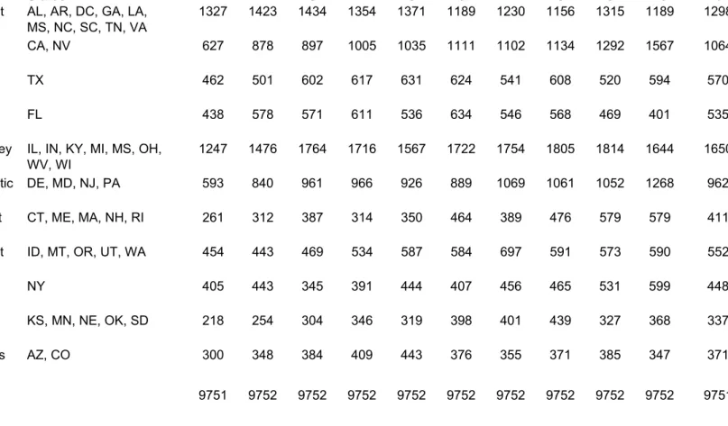
The population sampled in the survey includes 97,519 observations for 39,839 households; an observation equals one household in one quarter (Table 1).6 The Bureau
6 These numbers exclude observations in Hawaii and Alaska. Although households can remain in the data
for up to four quarters, each quarter’s sample is designed to be independently representative. Analysis has shown that richer, older, homeowning households are disproportianately likely to complete all four quarters of the survey. For both of these reasons, we treat each individual quarter as an observation, which we annualize, as opposed to only taking observations that contain four quarters’ worth of data.
of Labor Statistics (BLS) builds a national sample, and we use their data to construct national after-tax income deciles, also shown in Table 1.7 Since we are interested in a
finer level of geographic detail, we examine the data with state-level indicators. Because the BLS cannot preserve the confidentiality of its respondents when samples get small, 15,486 observations (6,605) households have missing state identifiers. This top-coding causes five states to fall out of the data entirely. Consequently, for the regional
component of our analysis, we have 82,033 observations for 33,234 households in 43 states plus the District of Columbia. We aggregate the observations into 11 regions.8
Observations with missing state identifiers are still used in our calculations at the national level.
7 We distribute regional observations based on the CEX data into these national income deciles. It is
important to keep in mind that these income “buckets” do not necessarily accurately represent regional income deciles; rather, they are constructed as deciles at the national level.
8 BLS refers to observations as “consumer units,” which we loosely interpret as households. The five
Table 1. Observations by Region and After-Tax Income Decile Decile
Region States 1 2 3 4 5 6 7 8 9 10 Total
Southeast AL, AR, DC, GA, LA, MS, NC, SC, TN, VA
1327 1423 1434 1354 1371 1189 1230 1156 1315 1189 12988
CNV CA, NV 627 878 897 1005 1035 1111 1102 1134 1292 1567 10648
TX TX 462 501 602 617 631 624 541 608 520 594 5700
FL FL 438 578 571 611 536 634 546 568 469 401 5352
Ohio Valley IL, IN, KY, MI, MS, OH, WV, WI
1247 1476 1764 1716 1567 1722 1754 1805 1814 1644 16509 Mid-Atlantic DE, MD, NJ, PA 593 840 961 966 926 889 1069 1061 1052 1268 9625 Northeast CT, ME, MA, NH, RI 261 312 387 314 350 464 389 476 579 579 4111 Northwest ID, MT, OR, UT, WA 454 443 469 534 587 584 697 591 573 590 5522
NY NY 405 443 345 391 444 407 456 465 531 599 4486
Plains KS, MN, NE, OK, SD 218 254 304 346 319 398 401 439 327 368 3374
Mountains AZ, CO 300 348 384 409 443 376 355 371 385 347 3718
The data for some expenditure categories appear missing or are reported as zero for a few households. Most problematic are reported zeros for electricity expenditures because while it is feasible that households do not pay a separate bill, in those cases they inevitably receive services bundled with their housing. Therefore our estimates may underestimate electricity expenditure. On the other hand, zero expenditure for gasoline for personal transportation is plausible, but also could reflect errors in data. We interpret the data as a conservative (lower bound) estimate of energy use and associated CO2
emissions in these categories.
As noted above, the transportation sector is given special consideration because of the new CAFE standards proposed by the Department of Transportation’s National Highway Traffic Safety Administration in April 2008 in response to the Energy Security and Independence Act passed in December 2007. These standards would bring the fuel economy standard for cars to 35.7 miles per gallon (mpg) and trucks to 28.6 mpg by the 2015 model year (Table 2).
Table 2. National Highway Traffic Safety Administration Proposed CAFÉ Standards
Model Year Cars, mpg Trucks, mpg
2011 31.2 25.0 2012 32.8 26.4 2013 34.0 27.8 2014 34.8 28.2 2015 35.7 28.6
The new regulations affect our baseline 2015 expenditure calculations in two ways. First, new vehicles are more costly than they would otherwise be and more costly than what is reflected in the 2006 CEX data, all else equal. Second, gasoline
expenditures, all else equal, are lower than they would be without the new standards (and lower than 2006). Since vehicles are a durable good, new, more fuel-efficient vehicles only gradually replace older, less efficient ones. We briefly describe our assumptions about how the stock turns over and how the new regulations affect our expenditure calculations.
More expensive vehicles. According to data from the Bureau of Transportation Statistics, the percentage of new car sales out of total registered cars in a given year is 5.7 percent, and the percentage of new trucks is 7.6 percent.9 We use these figures to
gradually increase the proportion of vehicles on the road that meet the new standards and we rely on estimates in Fischer et al. (2007) to obtain our higher vehicle price for those new vehicle purchases.10 A new car in 2015, meeting the 35.7 mpg standard, will cost
$149 more than it would in 2006, all else equal; a new truck will cost $246 more. In order to account for these cost increases, we have increased new vehicle costs by this amount in the base case.
Lower gasoline consumption. The gradual vehicle turnover leads to improvements in on-road fleetwide average fuel efficiency. We estimate that in 2015, the average fuel efficiency of cars on the road will be 26.3 mpg, while the average for trucks will be 21.9 mpg. These are improvements of 17 percent and 22 percent, respectively, over the fleetwide average for cars and trucks in 2006.11
Although the higher average fuel economy for vehicles on the road reduces gasoline consumption, consumption does not fall in lock-step with the rise in miles per gallon because of what is known as the “rebound effect.” When fuel economy increases, the cost per mile of driving falls and in response, people drive more. The net change in gasoline consumption thus equals fuel savings on current mileage from a unit reduction in miles per gallon, less the extra fuel consumption from the increase in vehicle miles traveled. Based on recent estimates, we assume this rebound effect is 10 percent–that is, a 1 percent decrease in the cost per mile of driving leads to a 10 percent increase in
gasoline consumption (Small and Van Dender 2007; U.S. Department of Transportation 2008). As a result, assuming the implementation of the new CAFE standards, gradual turnover in the vehicle stock, and the 10 percent rebound effect, average gasoline expenditures per household in 2015 are estimated to be 15 percent lower than the 2006 levels.
9 These are the figures for 2005, the most recently available data. See
http://www.bts.gov/publications/national_transportation_statistics/. The rate of replacement for new car and truck sales could also be affected by CAFE standards and the rising price of fuel that is not the result of carbon policy.
10 Fischer et al. (2007) rely on the National Academy of Sciences’ (2002) study of fuel economy
technologies for their estimates of the costs of meeting higher CAFE requirements.
11 On-road average fuel efficiency is available from the Bureau of Transportation Statistics. See
Figure 1. National Direct Energy Expenditures as a Fraction of Income
0.0
0.1
0.2
0.3
Fuel Oil Natural Gas Gasoline ElectricityFigure 1 illustrates the direct annual expenditures as a percentage of reported annual income by expenditure category at the national level. The 10 vertical bars represent income deciles, and the amount of expenditure in various categories, as a
percentage of income, is displayed for the average household within each decile. The four reported categories represent direct purchase by the average household of electricity, gasoline, natural gas, and heating oil. Consumption of each leads directly to CO2
emissions and climate policy would directly increase their cost.
At the national level, direct expenditure on energy represents 25.5 percent of annual income among the households in the lowest-income category, which is the
greatest percentage of any group. For the highest-income households it is 3.6 percent. On average across all income groups the share of expenditure on energy is 6.7 percent of annual income.
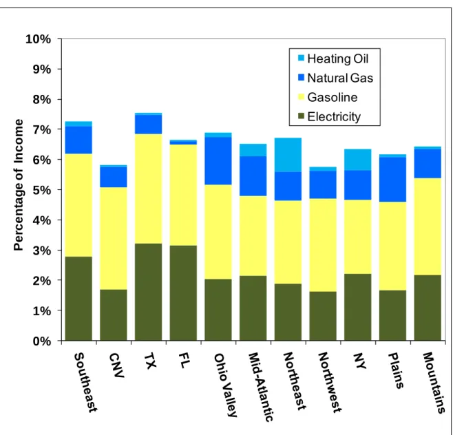
Figure 2. Average Household Expenditures by Region on Direct Fuel Purchases as Percentage of Income 0% 1% 2% 3% 4% 5% 6% 7% 8% 9% 10% Heating Oil Natural Gas Gasoline Electricity P e rc en ta g e o f In co m e
The nation is divided into 11 regions in our analysis. Figure 2 shows the average direct energy expenditures as a percentage of income in each region and for each fuel type. The average expenditure ranges from a low of 5.8 percent in California and Nevada and the Northwest to a high of 7.5 percent in Texas. In dollars, average annual
expenditures range from $3,547 in the Northwest to $4,676 in the Northeast.
These overall average direct expenditures do not show a great deal of variation across regions. This is consistent with the findings in Hassett et al. (2007). However,
when one looks at the distribution across income deciles for each region, some larger differences show up. As we stated above, the lowest decile has average direct
expenditures equal to 25.5 percent of income. This figure ranges from 22 percent in California and Nevada to 38.0 percent in the Northeast states, a difference of almost 14 percent. The ratio of expenditures as a fraction of income for the lowest decile to that for the highest is 11.5 in the Southeast—i.e., households in the lowest decile pay 11.5 times as much as those in the highest decile, as a percentage of income. In California and Nevada, the comparable figure is 7.7. These findings presage some of our policy scenario results in the next section of the paper.
The categories of expenditure also vary considerably across regions. Since the CO2 content of each type of expenditure varies, there would be variable effects on overall
expenditures across regions. In the Northeast and the Midatlantic area, home heating contributes importantly to expenditures, but not so in the South. In contrast, electricity expenditures are substantially greater as a percentage of income in the South than for other regions on average. Gasoline expenditures are also greatest in the South. The Midwest represents a sort of transition, with intermediate levels of expenditures in all categories. New York would also achieve levels as high as the other regions except for lower gasoline expenditures. In the West, overall expenditure tends to be lower, but gasoline expenditure is relatively high, especially compared with the Northeast. These variations are amplified when comparing regional differences for the lowest income groups.
To understand how household expenditures would be affected by climate policy, we calculate the quantities of fuels purchased by households in each group by taking expenditures from BLS and dividing by fuel-specific, state-specific energy prices from the Energy Information Administration (EIA). With information about the quantities of fuels purchased, we can calculate the embodied CO2 content of expenditures and the
incremental change in expenditures that would result from a price on CO2 emissions. For
natural gas, fuel oil, and gasoline, the carbon content and resulting CO2 emissions are
fixed numbers. For electricity, the CO2 content varies depending on the fuel used for
generation over seasonal and diurnal periods in different regions. This pattern is
identified from the Haiku electricity market model built and maintained by Resources for the Future.12
4.2 Estimating the Indirect CO2 Content of Other Expenditures The second category we incorporate in the analysis is spending on energy
embodied indirectly in goods and services, the most important of which are food, durable goods, and services. CO2 emissions resulting from indirect energy consumption are
calculated on the basis of data in Hassett et al. (2007), who provide information on the emissions intensity of goods aggregated into 38 indirect expenditure categories by updating methods developed in Metcalf (1999).13
The estimates of direct fuel use and the implied CO2 emissions based on the CEX
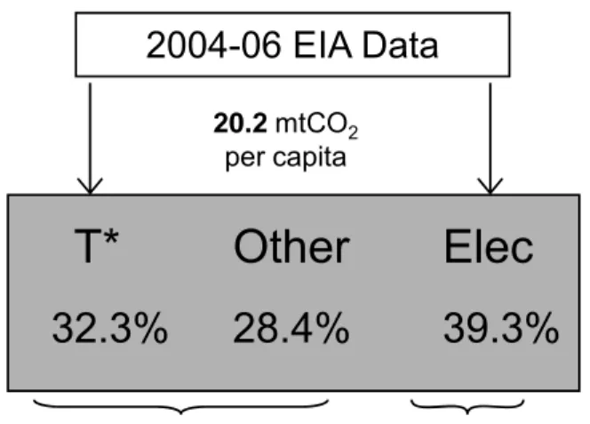
data correspond well to data collected by EIA (2007), as do those of Batz et al. (2007). However, the total emissions we calculate fall short of economywide EIA estimates. Our analysis of the CEX data accounts for per capita emissions of 16.9 metric tons CO2
(mtCO2), where information from EIA indicates per capita emissions of 20.2 mtCO2.14
Batz et al. (2007) mention several potential explanations for discrepancies between CEX data and other sources, including oversampling of urban areas in the CEX data. Another discrepancy is nonfossil fuel sources of CO2, including cement and limestone, which
account for nearly 2 percent in the EIA data but are missing from CEX data because input–output tables would not account for process emissions. Other possible sources of discrepancy are the estimate of the CO2 content of goods and services or errors in
mapping CEX data into expenditure categories. Finally, it is possible that this
discrepancy could reflect emissions from exports, which would show up in production data but not consumption data. However, the production data also would not account for emissions associated with the production of goods imported to the United States.
The literature reveals a variety of approaches to deal with inconsistency between the CEX data and other sources. Batz et al. (2007) correct for oversampling in their demographic model. Dinan and Rogers (2002) scale the CEX data so they align with expenditures reported in the National Income Product Accounts, which implicitly scales emissions from fossil fuel use at the national level. Boyce and Riddle (2007) do not scale and appear to account for only 13.46 mtCO2 per capita in their data. On the other hand,
Hassett et al. (2007) appear to account for emissions of 24.4 mtCO2 per capita, well
above the EIA estimate.
13 Hassett et al. (2007) provide information on the change in product price assuming no behavioral
adjustments in response to a tax of $15 per mtCO2. Dividing these price changes by 15 yields the implied
CO2 content per dollar spent in each category. Metcalf (1999) has been the basis for similar calculations
elsewhere in the literature (Dinan and Rogers 2002; Boyce and Riddle 2007).
ECONOMY
HOUSEHOLDS
Baseline
17.06 mtCO2 per capita2004-06 EIA Data
T*
Other
32.3%
28.4%
39.3%
2004-06 CEX Data
indirectt*
h
residential electric23%
51%
7%
19%
Hughes et al. Dahl indirectt*
h
residential electric22% 59% 9% 10%
Boyce & Riddle Haiku residential by region θe = -.13ε
= see textε
=-0.1Benchmark Policy
($41.50 mtCO2in 2015) 20.2 mtCO2 per capita20.2 mtCO2 per capita
(after scaling indirect)
Elec
ε
=-0.2* Baseline total and transportation (t) emissions do not reflect CAFE adjustment. Policy case does.
To measure the effects on households in a way that more closely resembles the EIA data, we scale the emissions intensity of nonfuel expenditures in the CEX data so that the total emissions correspond with EIA estimates. Therefore we only scale the emissions intensity of the indirect expenditure category, increasing it by 47 percent (3.31 mtCO2 per capita) to achieve overall EIA emissions levels.
The left side of Figure 3 reflects data and assumptions used in our analysis built on the CEX data. The upper left reports our estimate of 20.2 mtCO2 per capita after
scaling indirect expenditures. The upper boxes indicate our accounting for emissions in the baseline (no climate policy). The analysis of household expenditures on the left side of the figure includes percentages of emissions attributed to four categories of economic activity: personal transportation (t*), emissions from consumption of other goods and services after scaling so that total emissions match EIA (indirect), home heating with natural gas and fuel oil (h), and residential electricity. We discuss the elasticities and the benchmark policy results in Section 5 below.
The right side of Figure 3displays information about economywide emissions and the percentage of per capita emissions that are attributable to all transportation (T*), other sources (Other), and all electricity (Elec), according to EIA (2007). After adjusting for CAFE increases that will take effect by 2015 the emissions per capita fall from 20.2 to 19.52 mtCO2. We interpret this information as our baseline (no climate policy) average
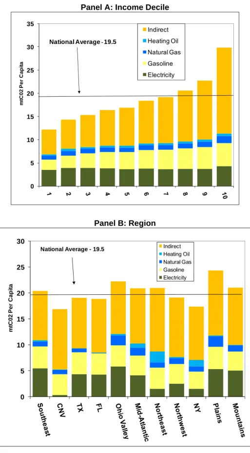
Figure 4. Emissions (mtCO2) per Capita by Alternative Measures
Panel A: Income Decile
0 5 10 15 20 25 30 35 Indirect Heating Oil Natural Gas Gasoline Electricity National Average-19.5 m tC 02 P e r C a p it a Panel B: Region 0 5 10 15 20 25 30 Indirect Heating Oil Natural Gas Gasoline Electricity National Average - 19.5 m tC 02 P e r C a p it a
Figure 4 (panel A) illustrates the CO2 content of expenditures for direct and
indirect fuel purchases for the average household in each income group at the national level. The expenditures for direct fuel purchases are distributed fairly evenly across income groups. The big difference emerges in the indirect expenditure category where high income households spend significantly more than low income households. We assume the emissions intensity per dollar of expenditure for indirect consumption of fuels is uniform throughout the country; consequently, actual emissions vary directly with expenditure. However, panel B in Figure 4 shows that there are significant differences across regions in the types of direct expenditures for fuels. The variation in emissions from the electricity sector is particularly noteworthy.
5 Effects of Pricing CO2
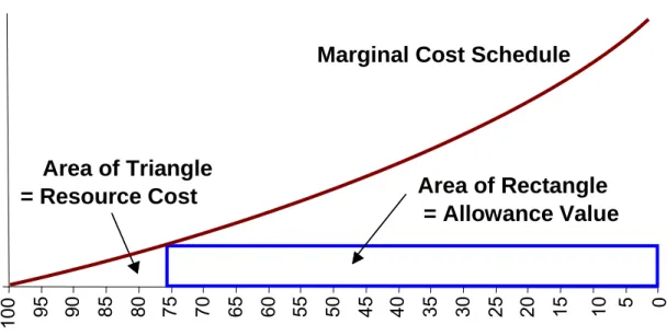
Figure 5 illustrates the mechanism of a placing a price on CO2 emissions through
the introduction of a cap-and-trade policy. The horizontal axis in the graph is the reduction in emissions (moving to the right implies lower emissions), and the upward sloping curve is the incremental resource cost of a schedule of measures to reduce emissions; thus it sketches out the marginal abatement cost curve. The hypothetical emissions cap in the figure is set at about 75 percent of baseline emissions. According to most experts, for the next couple of decades at least, the value of emissions allowances under a cap-and-trade program should be substantially larger than the value of the
resources actually used to achieve emissions reductions. This relationship is illustrated in the stylized graph, where the allowance value rectangle—the height of the rectangle equals the allowance price and the width is the number of emissions allowances—is much larger than the triangle-shaped abatement costs. Moreover, the value of the allowances (the rectangle) grows faster than the cost of emissions reductions (the
triangle) as the emissions cap is tightened until reductions of about one-third are reached. These facts highlight the important role played by the allocation of emissions allowances in determining the regressivity of climate policy under an incentive-based policy such as cap-and-trade or a carbon tax.
Figure 5. Resource Cost and Allowance Value in a CO2 Cap-and-Trade Program
An emissions cap-and-trade program (or equivalently an emissions tax) serves as a central policy case to provide a benchmark for our comparison of policies. We
benchmark the stringency to an emissions reduction of 3.13 mtCO2 per capita, including
the CAFE adjustment, resulting from a price of $41.50 (in 2006 dollars) per ton of CO2.15
We assume the policy is announced in 2008 and takes effect in 2012, and we consider the effect on households in 2015. This time frame allows for some technological evolution in transportation and electricity; otherwise, expenditure patterns of households are assumed to match those in the CEX data. In evaluating alternative policies that could be pursued to address distributional effects we scale the CO2 price in order to hold per capita emissions
constant so that these alternatives can be compared with the benchmark climate policy in an emissions-neutral manner.
To calculate the change in emissions we multiply the CO2 price by the CO2
content of expenditures in each category except electricity and add this to the product
15 This price reflects a marginal cost approximately three times greater than what would have been
expected from the McCain–Lieberman proposal (S.280) and is roughly equal to the price of emissions allowances in the E.U. Emissions Trading Scheme for the second trading period (2008–2012), which were
10 0 95 90 85 80 75 70 65 60 55 50 45 40 35 30 25 20 15 10 5 0 Percent of Emissions D o llars
Area of Rectangle
= Allowance Value
Marginal Cost Schedule
Area of Triangle
= Resource Cost
10 0 95 90 85 80 75 70 65 60 55 50 45 40 35 30 25 20 15 10 5 0 Percent of Emissions D o llarsArea of Rectangle
= Allowance Value
Marginal Cost Schedule
Area of Triangle
= Resource Cost
price to calculate new levels of expenditure. Although demand is relatively inelastic in the short run, the change in product prices is expected to lead to a change in consumer expenditures, which we calculate using elasticity estimates specific to each fuel. As reported in the left side of Figure 3, we use short-run elasticity
( )
ε for gasoline of –0.1 taken from Hughes et al. (2008). For indirect expenditures, we use several short-run elasticities take from Boyce and Riddle (2007) that range from –0.25 to –1.3.16 Fornatural gas we use –0.2 taken from Dahl (1993); we also use this elasticity for fuel oil. To model the change in residential electricity demand we use the Haiku model, which solves for equilibria including changes in investment in generation capacity, electricity price, and demand at the regional level. The change in carbon emissions (mtCO2) for residential
customers in the electricity sector for a $1.00 change in the carbon price is Θ = −e 0.13. These estimates allow us to calculate the new quantity of consumption, which can be multiplied by the new price to find the new level of expenditures. The net effect of these changes in expenditures is an emissions level of 17.06 mtCO2 per capita. With an eye on
changes that would be likely to occur by 2015, the use of short-run elasticities is probably appropriate; however, it may underrepresent the behavioral changes that would occur under climate policy as more adjustments could be made in the seven-year time period.
This approach implicitly assumes all changes in costs are fully passed through to consumers in every industry except electricity, which we model in greater detail. In the long run, production technology is usually characterized as constant returns to scale, which implies that consumers bear the cost of policy. In the short run there is more likely to be a sharing of lost economic surplus with producers because of changes in the value of in-place capital, but this will dissipate over time. The electricity sector is an exception because of the long-lived nature of capital in the sector, which means that the loss to producers will dissipate more slowly. Nonetheless, even in this sector consumers are expected to bear eight times the cost born by producers.17 The degree to which the
burden of any tax is shared between consumers and producers has been the focus of previous studies but is outside our scope here. As explained in the literature review above, Holak (2008) assesses the distributional impacts of a carbon tax under alternative assumptions about the share of burden borne by consumers and producers.
16 These indirect elasticities are –0.6 for food; –1.3 for industrial goods; –1 for services; and –0.25 for air
and other transport.
5.1 How to Interpret Incidence and Alternative Policy Remedies
The $41.50 CO2 price that we model in the benchmark policy case is expected to
yield a reduction of 16 percent in CO2 emissions per capita according to our model of
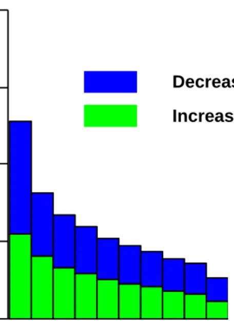
household expenditures. Figure 6 illustrates the distribution of costs over income groups at the national level after accounting for changes in expenditures. To understand the numbers in Figure 6, consider an average family in the fifth decile. If one were to ignore the change in consumption that would be expected, as has been done in much of the previous literature, then the introduction of the CO2 price would cause expenditures for
direct energy use to increase by $807 (1.9 percent) and total expenditures to increase by $1,711 (4.1 percent). However, after accounting for changes in consumption behavior in response to the higher prices, this family would experience an increase in expenditures of only $868 (2.1 percent), which is indicated by the smaller bar in the figure. This does not account for the revenue from allowances; it is simply an illustration of how expenditures for direct fuel use and for consumption of goods and services with indirect emissions would change if the prices were to reflect the price of allowances, accounting for behavioral responses in each market as described previously. The figure illustrates that the changes as a percentage of income appear the greatest for low-income households because they spend proportionately more on energy-related expenditures.
Figure 6. Expenditures and Consumer Surplus Loss as Fraction of Income by Income Decile
.00
.04
.08
.12
.16
Decrease in Consumer Surplus Increase In Expenditure
The change in expenditure can differ importantly from the change in consumer surplus. To illustrate the differences between the two measures, imagine an expenditure category with own-price elasticity of demand equal to –1. In this case, an increase in price would lead to a reduction in quantity but there would be no change in expenditure. Simply equating expenditure change with well-being therefore would underestimate the cost of constraining carbon; all other things equal, consumers are clearly harmed if they are forced to consume less. The larger quantities in the bar graph in Figure 6 indicate the changes in consumer surplus as a percentage of income; the change in consumer surplus is always larger than the change in expenditure. Positive values indicate the absolute value of the magnitude of the loss. Again, the greatest changes (loss in consumer surplus) as a percentage of income occur for low-income households. 18
One way to represent the distribution of costs in a quantitative manner is the Suits Index, which is the tax analog to the better-known Gini coefficient that serves as an index measuring income inequality. A curve is constructed by plotting the relationship between cumulative tax paid and cumulative income earned.19 The area under this curve is then
compared with the area under a proportional line to calculate the Suits Index. If all tax collections are nonnegative, the index is bounded by –1 and 1, with values less than zero connoting regressivity and values greater than zero connoting progressivity; a
proportional tax has a Suits Index of zero (Suits 1977). The Suits Index provides a simple metric with which to compare the distributional impacts of alternative policies. We modify the standard interpretation to measure the incidence on households according to their loss in consumer surplus rather than taxes paid. Second, we allow for negative tax payments and other forms of subsidies, so our modified Suits Index (MSI) is not bounded by –1 and 1. At the national level, not accounting for the revenue that may be collected or the allocation of emissions allowances, the MSI value for the CO2 price of $41.50 is
-0.18.
18 West (2004) showed that when demand elasticities vary by income group, using consumer surplus
rather than expenditures can lead to quite different distributional findings. She estimates a more elastic demand for gasoline (and miles traveled) in lower-income groups than higher ones, leading those groups to reduce gasoline expenditures more in response to a gasoline tax (and other vehicle-related taxes). This behavioral adjustment will mute the regressivity of the tax when regressivity is measured on the basis of expenditures. However, the consumer surplus effect, because it adds a welfare loss triangle to the expenditure rectangle, indicates a greater harm to lower-income households. Although we calculate a consumer surplus effect, we do not allow elasticities to vary by income.
19 This curve is similar to a Lorenz curve, which graphically represents the cumulative distribution of
The impact of the policy on household direct energy expenditures differs across regions, as evident in Figure 2, and we also find differences with respect to changes in expenditure on goods and services that are affected by the CO2 price. Hassett et al. (2007)
conduct a comparison of the regional incidence of a carbon tax, finding it “quite remarkable how small” the differences are across regions. Batz et al. (2007) reach a different conclusion. Although they only look at direct energy use, they do so with much greater geographic detail than previous efforts by looking at data at the county level, and they look at differences in the emissions intensity of electricity generation across the country. They find “substantial variation in the incidence of a carbon emissions tax” across regions, which they explain as due to variation in energy use as well as differences in the carbon intensity of electricity generation. Our analysis does not have the detail at the county level, but it does have similar estimates of electricity generation by using an updated version of the model they use, and it includes indirect expenditures. These analyses do not look at the allocation of CO2 revenue.
The $41.50 CO2 price raises significant revenue that must be accounted for in
some manner. We assume the first claimant for the revenue is government, which is subject to a budget constraint. The government budget is affected in at least three ways (Dinan and Rogers 2002). One is that government’s energy-related expenses would increase under climate policy. Second, if the policy leads to a reduction in overall spending, government would see a decline in revenues from taxation. Third, the government could see an increase in the cost of social programs if the economy slows down as a consequence of the policy or if lower-income households are severely affected. Finally, we assume there will be an increase in government expenditures to fund climate-related research. To maintain the government’s budget constraint (at the federal and state level combined), throughout the following analysis we assume that 35 percent of the revenue collected is immediately directed to the government, leaving 65 percent of the revenue for other purposes.20 In some cases the climate policy could lead to additional
sources of government revenue such as taxes collected on extra dividends that result if free allocation of allowances were given to emitters. In the policy scenarios that follow, we net out this effect so that the government retains a constant 35 percent share of revenue in each scenario.
20 Dinan and Rogers (2002) estimate that the government would need about 23 percent of the allowance
value to offset its higher costs stemming from its own consumption of allowances, adjustments to higher energy prices, higher transfer income payments, lower revenues, and automatic indexing of individual tax
6 Results for Alternative Policy Scenarios
The price on CO2 emissions creates a sum of revenue of significant value. The
way this value is allocated to different groups in the economy greatly affects the costs and distributional burden of the carbon policy. Evaluating alternative approaches to the distribution of the CO2 revenue provides important information to policymakers trying to
design an efficient and fair policy. We group our revenue scenarios into (1) cap-and-dividend options, (2) changes to preexisting taxes, (3) energy and fuel sector adjustments, and as a comparison, (4) a scenario with free allocation to incumbent emitters.
Some of the approaches we analyze have “leftover” revenue because of the level at which we set the remedy or the type of remedy. When this is the case, we assume the leftover revenue is distributed in the same manner as cap-and-dividend, that is, in a lump sum manner to each person, so all approaches can be directly compared. In all cases, we assume the government captures the first 35 percent of CO2 revenue.
6.1 Cap-and-Dividend (Lump Sum Transfers)
One straight-forward remedy to alleviate the regressivity of the carbon policy would be to return the CO2 revenue to households on a per capita basis. This approach
recently has been referred to as “cap-and-dividend” (Boyce and Riddle 2007) and previously was known as “sky trust” (Kopp et al. 1999; Barnes 2001). In principle, the government would auction the emissions allowances and return the auction revenues in a lump sum manner to each person. Using information from the CEX, we identify the number of persons per household in each income group in each region and calculate a per capita dividend payment to redistribute to each household. In our first scenario, people are assumed to pay personal income taxes on the dividends. In the next scenario, discussed in section 6.1.ii below, we consider a dividend that is not taxed. 21
6.1.1 Taxed Dividends
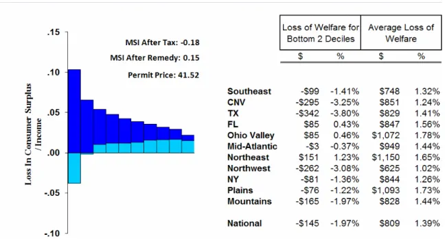
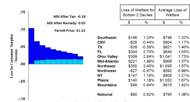
The net effect of the first cap-and-dividend policy, by region and nationally, is shown in Figure 7. The bar graph illustrates the incidence of the policy, in consumer surplus loss, on the average household in each income group; the table portion of the
21 Since our results are derived in a partial equilibrium setting, we do not consider any effects that this
lump sum payment would have on household expenditures. However, recent evidence from the behavioural economics literature suggests that consumers are unlikely to factor the expectation of such payments into their shortrun energy consumption decisions (Sunstein and Thaler 2008).
figure shows the impacts for the average household in each region and for the households in the lowest two income deciles. The MSI and the carbon allowance price are also listed.
Figure 7. Cap-and-Dividend (Taxable)
The bar with darker shading and the greatest vertical height represents the loss in consumer surplus as a share of after tax income. (This value repeats information that was illustrated in Figure 6). The bar with the lighter shading represents the incidence of the policy after distributing the value of allowances as a per capita dividend. The first finding that is obvious from the graph is the fact that households in the lowest deciles see a dramatic improvement in their well-being as a result of the lump sum dividend of allowance revenues. The average household in decile 1 incurs a consumer surplus loss slightly greater than 10 percent of its income without the dividend but gets a consumer surplus gainequal to 3.8 percent of income with the dividend.
The second interesting result is that the dividend equalizes the net burden across income groups. The net consumer surplus loss as a percentage of income across deciles 2 through 10 ranges from approximately zero for decile 2 to only 1.68 percent for decile 9. These results highlight the fact that the dividend, as a percentage of income, obviously has a much greater impact for poorer households than for wealthier ones. The MSI reinforces these findings: as stated above, the MSI for the carbon pricing policy alone (without the redistribution of allowance revenues) is –0.18; the MSI with the (taxed)
lump sum redistribution of revenues is 0.15. Thus the policy goes from being regressive to mildly progressive.
The table portion of Figure 7 shows the net dollar loss in consumer surplus (including the dividend), along with the loss as a percentage of income, for an average household in each region and for an average household in deciles 1 and 2. (Positive numbers in the table indicate a loss and negative numbers indicate a gain, consistent with the graph.) The important take-away message from the numbers in the table is the
significant variation in impacts across regions for households in deciles 1 and 2. In Texas, these households experience a consumer surplus gain of $342, or 3.8 percent of income, while households in deciles 1 and 2 in the Northeast incur a loss of $151, or 1.23 percent of income. By contrast, the variation for the mean household across regions is relatively small when viewed as a percentage of income—the lowest region is the Northwest, with a loss equal to approximately 1 percent of income, while the highest is the Ohio Valley at 1.78 percent.
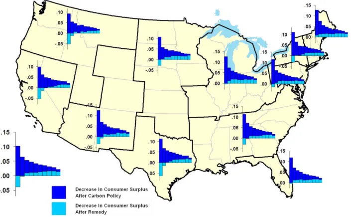
Figure 8. Cap-and-Dividend (Taxable)
To illustrate the incidence of policy across all income groups and regions we display a map in Figure 8. Again, the bars with darker shading and the greatest vertical
height represent the loss in consumer surplus as a share of after-tax income, and the bars with the lighter shading represent the net loss after distributing the value of allowances as a per capita dividend. The figure for the nation is replicated in the lower-left corner, and the region-specific figures are displayed for each of the 11 regions we model. The map indicates that the regional differences come into consideration for the lower-income groups and for the average consumers. There is relatively little variation among the upper-income groups across regions.
6.1.2 Nontaxable Dividends
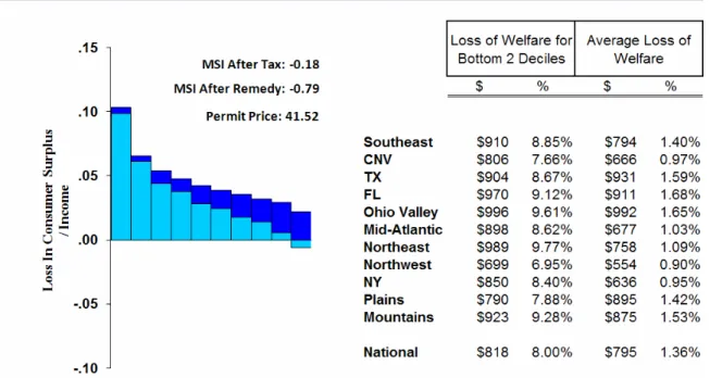
It is not clear whether carbon allowance dividends in a new cap-and-trade
program would be treated as taxable or nontaxable income. Our first scenario considered them as taxable, the same as most other sources of income. In other words, the
government was assumed to collect the allowance revenue and redistribute the entire amount (less the 35 percent that is withheld in all our scenarios) to households that would then pay taxes on that money at their standard marginal rate. In this scenario, we treat the dividends as untaxed. This case is similar to the 2008 federal tax rebates, which were also untaxed.
Figure 9. Cap-and-Dividend (Nontaxable)