Rethinking Database Algorithms for Phase Change Memory

(1)

Rethinking Database Algorithms for

Phase Change Memory

Shimin Chen

Intel Labs Pittsburgh

Phillip B. Gibbons

Intel Labs Pittsburgh

Suman Nath

Microsoft Research

ABSTRACT

Phase change memory (PCM)is an emerging memory tech-nology with many attractive features: it is non-volatile, byte-addressable, 2–4X denser than DRAM, and orders of magnitude better than NAND Flash in read latency, write latency, and write endurance. In the near future, PCM is expected to become a common component of the mem-ory/storage hierarchy for a wide range of computer systems. In this paper, we describe the unique characteristics of PCM, and their potential impact on database system design. In particular, we present analytic metrics for PCM endurance, energy, and latency, and illustrate that current approaches for common database algorithms such as B+_{-trees and Hash}

Joins are suboptimal for PCM. We present improved algo-rithms that reduce both execution time and energy on PCM while increasing write endurance.

1. INTRODUCTION

Phase change memory (PCM)[3, 10] is an emerging non-volatile memory technology with many attractive features. Compared to NAND Flash, PCM provides orders of mag-nitude better read latency, write latency and endurance,1

and consumes significantly less read/write energy and idle power [9, 10]. It is byte-addressable, like DRAM mem-ory, but consumes orders of magnitude less idle power than DRAM. PCM offers a significant density advantage over DRAM, which means more memory capacity for the same chip area and also implies that PCM is likely to be cheaper than DRAM when produced in mass market quantities [22]. While the first wave of PCM products target mobile hand-sets [24], in the near future PCM is expected to become a common component of the memory/storage hierarchy for laptops, PCs, and servers [9, 15, 22].

An important question, then, ishow should database sys-tems be modified to best take advantage of this emerging

1

(Write) enduranceis the maximum number of writes for each memory cell.

This article is published under a Creative Commons Attribution License (http://creativecommons.org/licenses/by/3.0/), which permits distribution and reproduction in any medium as well allowing derivative works, pro-vided that you attribute the original work to the author(s) and CIDR 2011. 5th Biennial Conference on Innovative Data Systems Research (CIDR ’11) January 9-12, 2011, Asilomar, California, USA.

trend towards PCM? While there are several different pro-posals for how PCM will fit within the memory hierarchy [10] (as SATA/PCIe based data storage or DDR3/QPI based memory), recent computer architecture and systems studies all propose to incorporate PCM as the bulk of the system’s main memory [9, 15, 22]. Thus, in the PCM-DB project [19], we are focusing on the use of PCM as the primary main memory for a database system. This paper highlights our initial findings and makes the following three contributions. First, we describe the unique characteristics of PCM and its proposed use as the primary main memory (Section 2). Several attractive properties of PCM make it a natural can-didate to replace or compliment battery-backed reliable mem-ory for general database systems [18], and DRAM in main memory database systems [11]. However, a unique chal-lenge arises in effectively using PCM: Compared to its read operations, PCM writes incur higher energy consumption, higher latency, lower bandwidth, and limited endurance. Therefore, we identify reducing PCM writes as an impor-tant design goal of PCM-friendly algorithms. Note that this is different from the goals of flash-friendly algorithms [2, 17], which include reducing the number of erasesand ran-dom writesat muchcoarsergranularity (e.g., 256KB erase blocks and 4KB flash pages).

Second, we present analytic metrics for PCM endurance, energy, and latency. While we believe that PCM may have a broad impact on database systems in general, this pa-per focuses on its impact on core database algorithms. In particular, we use these metrics to design PCM-friendly al-gorithms for two core database techniques, B+_{-tree index}

and hash joins (Section 3). In a nutshell, these algorithms re-organize data structures and trade off an increase in PCM reads for reducing PCM writes, thereby achieving an overall improvement in all three metrics.

Third, we show experimentally, via a cycle-accurate X86-64 simulator enhanced with PCM support, that our new al-gorithms significantly outperform prior alal-gorithms in terms of time, energy and endurance (Section 4), supporting our analytical results. Moreover, sensitivity analysis shows that the results hold for a wide range of PCM parameters.

The paper concludes by discussing related work (Section 5) and highlighting a few of the many interesting open research questions regarding the impact of PCM main memory on database systems (Section 6).

2. PHASE CHANGE MEMORY

In this section, we discuss PCM technology, its properties relative to other memory technologies, its proposed use as

(2)

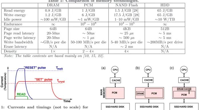
Table 1: Comparison of memory technologies.

DRAM PCM NAND Flash HDD

Read energy 0.8 J/GB 1 J/GB 1.5 J/GB [28] 65 J/GB Write energy 1.2 J/GB 6 J/GB 17.5 J/GB [28] 65 J/GB Idle power ∼100 mW/GB ∼1 mW/GB 1–10 mW/GB ∼10 W/TB Endurance ∞ 106 −108 104 −105 ∞ Page size 64B 64B 4KB 512B

Page read latency 20-50ns ∼50ns ∼25µs ∼5 ms

Page write latency 20-50ns ∼1µs ∼500µs ∼5 ms

Write bandwidth ∼GB/s per die 50-100 MB/s per die 5-40 MB/s per die ∼200MB/s per drive

Erase latency N/A N/A ∼2 ms N/A

Density 1× 2−4× 4× N/A

Note: The table contents are based mainly on [10, 15, 22].

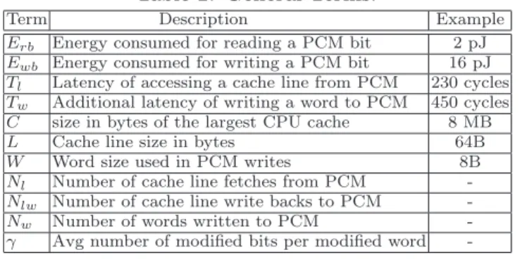
"RESET" pulse "SET" pulse READ Time (Temperature) Current cryst melt T T

Figure 1: Currents and timings (not to scale) for SET, RESET, and READ operations on a PCM cell. For phase change materialGe2Sb2T e5, Tmelt ≈610◦C

andTcryst≈350◦C.

the primary main memory, and the key challenge of over-coming its write limitations.

2.1 PCM Technology

Phase change memory (PCM) is a byte-addressable non-volatile memory that exploits large resistance contrast be-tween amorphous and crystalline states in so-called phase change materials such as chalcogenide glass. The difference in resistance between the high-resistance amorphous state and the low-resistance crystalline state is typically about five orders of magnitude and can be used to infer logical states of binary data (high represents 0, low represents 1).

Programming a PCM device involves application of elec-tric current, leading to temperature changes that either SET or RESET the cell, as shown schematically in Figure 1. To SET a PCM cell to its low-resistance state, an electrical pulse is applied to heat the cell above the crystalization tem-peratureTcryst(but below the melting temperatureTmelt) of

the phase change material. The pulse is sustained for a suffi-ciently long period for the cell to transition to the crystalline state. On the other hand, to RESET the cell to its high-resistance amorphous state, a much larger electrical current is applied in order to increase the temperature aboveTmelt.

After the cell has melted, the pulse is abruptly cut off, caus-ing the melted material to quench into the amorphous state. To READ the current state of a cell, a small current that does not perturb the cell state is applied to measure the resistance. At normal temperatures (< 120◦_C _≪ _T

cryst),

PCM offers many years of data retention.

2.2 Using PCM in the Memory Hierarchy

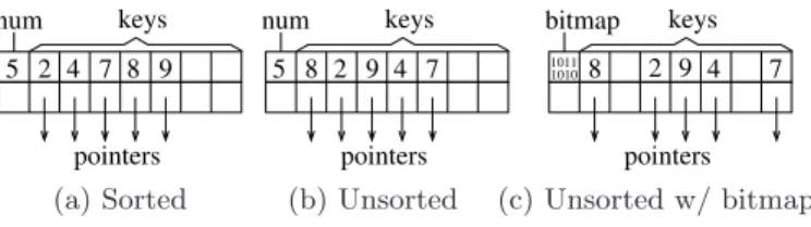
To see where PCM may fit in the memory hierarchy, we need to know its properties. Table 1 compares PCM with DRAM (technology for today’s main memory), NAND flash

SSD/HARD DISK MEMORY MAIN CACHE PCM CPU (a) CACHE SSD/HARD DISK CPU DRAM PCM (b) CACHE SSD/HARD DISK DRAM CACHE CPU PCM (c)

Figure 2: Candidate main memory organizations with PCM.

(technology for today’s solid state drives), and HDD (hard disk drives), showing the following points:

• Compared to DRAM, PCM’s read latency is close to that of DRAM, while its write latency is about an order of magnitude slower. PCM offers a density ad-vantage over DRAM. This means more memory capac-ity for the same chip area, or potentially lower price per capacity. PCM is also more energy-efficient than DRAM in idle mode.

• Compared to NAND Flash, PCM can be programmed in place regardless of the initial cell states (i.e., with-out Flash’s expensive “erase” operation). Therefore, its sequential and random accesses show similar (far superior) performance. Moreover, PCM has orders of magnitude higher write endurance than Flash. Because of these attractive properties, PCM is being incor-porated in mobile handsets [24], and recent computer ar-chitecture and systems studies have argued that PCM is a promising candidate to be used in main memory in future mainstream computer systems [9, 15, 22].

Figure 2 shows three alternative proposals in recent stud-ies for using PCM in the main memory system [9, 15, 22]. Proposal (a) replaces DRAM with PCM to achieve larger main memory capacity. Even though PCM is slower than DRAM, clever optimizations have been shown to reduce ap-plication execution time on PCM to within a factor of 1.2 of that on DRAM [15]. Both proposals (b) and (c) include a small amount of DRAM in addition to PCM so that fre-quently accessed data can be kept in the DRAM buffer to improve performance and reduce PCM wear. Their differ-ence is that proposal (b) gives software explicit control of the DRAM buffer [9], while proposal (c) manages the DRAM

(3)

buffer as another level of transparent hardware cache [22]. It has been shown that a relatively small DRAM buffer (3% size of the PCM storage) can bridge most of the latency gap between DRAM and PCM [22].

2.3 Challenge: Writes to PCM Main Memory

One major challenge in effectively using PCM is overcom-ing the relative limitations of its write operations. Com-pared to its read operations, PCM writes incur higher energy consumption, higher latency, lower bandwidth, and limited endurance, as discussed next.

• High energy consumption: Compared to reading a PCM cell, a write operation that SETs or RESETs a PCM cell draws higher current, uses higher voltage, and takes longer time (Figure 1). A PCM write often con-sumes 6–10X more energy than a read [15].

• High latency and low bandwidth: In a PCM device, the write latency of a PCM cell is determined by the (longer) SET time, which is about 3X slower than a read operation [15]. Moreover, many PCM prototypes support “iterative writing” of a limited number of bits per iteration in order to limit the instantaneous cur-rent level. Several prototypes support×2,×4, and×8 write modes in addition to the fastest×16 mode [3]. This limitation is likely to hold in the future as well, es-pecially for PCM designed for power-constrained plat-forms. Because of the limited write bandwidth, ing 64B of data often requires several rounds of writ-ing, leading to the∼1µs write latency in Table 1. • Limited endurance: Existing PCM prototypes have a

write endurance ranging from 106

to 108

writes per cell. With a good wear-leveling algorithm, a PCM main memory can last for several years under realistic workloads [21]. However, because such wear-leveling must be done at the memory controller, the wear-leveling algorithms need to have small memory foot-prints and be very fast. Therefore, practical algo-rithms are simple and in many cases, their effective-ness significantly decreases in the presence of extreme hot spots in the memory. For example, even with the wear-leveling algorithms in [21], continuously updat-ing a counter in PCM in a 4GHz machine with 16GB PCM could wear a PCM cell out in about 4 months (without wear-leveling, the cell could wear out in less than a minute).

Recent studies proposed various hardware optimizations to reduce the number of PCM bits written [8, 15, 31, 32]. For example, the PCM controller can perform data com-parison writes, where a write operation is replaced with a read-modify-write operation in order to skip programming unchanged bits [31]. Another proposal ispartial writes for only dirty words [15]. In both optimizations, when writ-ing a chunk of data in multiple iterations, the set of bits to write in every iteration is often hard-wired for simplicity; if all the hard-wired bits of an iteration are unchanged, the iteration can be skipped [7]. However, these architectural optimizations reduce the volume of writes by only a fac-tor∼3. We believe that applications (such as databases) can play an important role in complementing such architec-tural optimizations by carefully choosing their algorithms and data structures in order to reduce the number of writes, even at the expense of additional reads.

Table 2: General Terms.

Term Description Example

Erb Energy consumed for reading a PCM bit 2 pJ

Ewb Energy consumed for writing a PCM bit 16 pJ

Tl Latency of accessing a cache line from PCM 230 cycles

Tw Additional latency of writing a word to PCM 450 cycles

C size in bytes of the largest CPU cache 8 MB

L Cache line size in bytes 64B

W Word size used in PCM writes 8B

Nl Number of cache line fetches from PCM

-Nlw Number of cache line write backs to PCM

-Nw Number of words written to PCM

-γ Avg number of modified bits per modified word

-3.

PCM-FRIENDLY DB ALGORITHMS

In this section, we consider the impact of PCM on database algorithm design. Specifically, reducing PCM writes be-comes an important design goal. We discuss general con-siderations in Section 3.1. Then we re-examine two core database techniques, B+

-tree index and hash joins, in Sec-tions 3.2 and 3.3, respectively.

3.1 Algorithm Design Considerations

Section 2 described three candidate organizations of fu-ture PCM main memory, as shown in Figure 2. Their main difference is whether or not to include a transparent or software-controlled DRAM cache. For algorithm design pur-poses, we consider an abstract framework that captures all three candidate organizations. Namely, we focus on a PCM main memory, and view any additional DRAM as just an-other (transparent or software-controlled) cache in the hier-archy. This enables us to focus on PCM-specific issues.

Because PCM is the primary main memory, we consider algorithm designs in main memory. There are two tradi-tional design goals for main memory algorithms: (i) low computation complexity, and (ii) good CPU cache perfor-mance. Power efficiency has recently emerged as a third design goal. Compared to DRAM, one major challenge in designing PCM-friendly algorithms is to cope with the asym-metry between PCM reads and PCM writes: PCM writes consume much higher energy, take much longer time to com-plete, and wear out PCM cells (recall Section 2). Therefore, one important design goal of PCM-friendly algorithms is to minimize PCM writes.

What granularity of writes should we use in algorithm analysis with PCM main memory: (a) bits, (b) words, or (c) cache lines? All three granularities are important for com-puting PCM metrics. Choice (a) impacts PCM endurance. Choices (a) and (c) affect PCM energy consumption. Choice (b) influences PCM write latency. The drawback of choice (a) is that the relevant metric is the number of modified bits (recall that unmodified bits are skipped); this is dif-ficult to estimate because it is often affected not only by the structure of an algorithm, but also by the input data. Fortunately, there is often a simple relationship between (a) and (b). Denoteγ as the average number of modified bits per modified word. γ can be estimated for a given input. Therefore, we focus on choices (b) and (c).

LetNl (Tl) be the number (latency, resp.) of cache line

fetches (a.k.a. cache misses) from PCM, Nlw be the

num-ber of cache line write backs to PCM, andNw (Tw) be the

number (latency, resp.) of modified words written. LetErb

(Ewb) be the energy for reading (writing, resp.) a PCM bit.

(4)

sum-marizes the notation used in this paper.) We model the key PCM metrics as follows:

• TotalWear: N umBitsM odif ied=γNw

• Energy= 8L(Nl+Nlw)Erb+γNwEwb

• T otalP CM AccessLatency=NlTl+NwTw

The total wear and energy computations are straightfor-ward. The latency computation requires explanations. The first part (NlTl) is the total latency of cache line fetches

from PCM. The second part (NwTw) is the estimated

im-pact of cache line write backs to PCM on the total time. In a traditional system, the cache line write backs are per-formed asynchronously in the background and often com-pletely hidden. Therefore, algorithm analysis typically ig-nores the write backs. However, we find that because of the asymmetry of writes and reads, PCM write latency can keep PCM busy for a sufficiently long time to stall front-end cache line fetches significantly. A PCM write consists of (i) a read of the cache line from PCM to identify modified words then (ii) writing modified words in possibly multiple rounds. The above computation includes (ii) asNwTw, while the latency

of (i) (NlwTl) is ignored because it is similar to a traditional

cache line write back and thus likely to be hidden.

3.2 B

+

_{-Tree Index}

As case studies, we consider two core database techniques for memory-resident data, B+

-trees (in the current subsec-tion) and hash joins (in the next subsecsubsec-tion), where the main memory is PCM instead of DRAM.

B+

-trees are preferred index structures for memory-resident data because they optimize for CPU cache performance. Previous studies recommend that B+

-tree nodes be one or a few cache lines large and aligned at cache line boundaries [5, 6, 12, 23]. For DRAM-based main memory, the costs of search/insertion/deletion are similar except in those cases where insertions/deletions incur node splits/merges in the tree. In contrast, for PCM-based main memory, even a nor-mal insertion/deletion that modifies a single leaf node can be more costly than a search in terms of total wear, energy, and elapsed time, because of the writes involved.

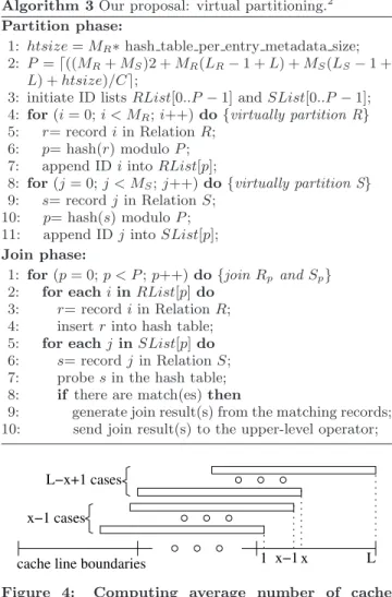
We would like to preserve the good CPU cache perfor-mance of B+

-trees while reducing the number of writes. A cache-friendly B+

-tree node is typically implemented as shown in Figure 3(a), where all the keys in the node are sorted and packed, and a counter keeps track of the number of valid keys in the array. The sorted key array is maintained upon insertions and deletions. In this way, binary search can be applied to locate a search key. However, on average, half of the array must be moved to make space for insertions and deletions, resulting in a large number of writes. Sup-pose that there areKkeys andKpointers in the node, and every key, every pointer, and the counter have size equal to the word size W used in PCM writes. Then an inser-tion/deletion in the sorted node incurs 2(K/2) + 1 =K+ 1 word writes on average.

To reduce writes, we propose two simple unsorted node organizations as shown in Figures 3(b) and 3(c):

• Unsorted: As shown in Figure 3(b), the key array is still packed but can be out of order. A search has to scan the array sequentially in order to look for a match or the next smaller/bigger key. On the other hand, an insertion can simply append the new entry to

5 2 4 7 8 9 pointers keys num 5 8 2 9 4 7 pointers keys num pointers keys bitmap 8 2 9 4 7 1011 1010

(a) Sorted (b) Unsorted (c) Unsorted w/ bitmap Figure 3: B+

-tree node organizations. Table 3: Terms used in analyzing hash joins.

Term Description

MR,MS Number of records in relation R and S, respectively

LR,LS Record sizes in relation R and S, respectively

NhR Number of cache line accesses per hash table visit_{when building the hash table on R records}

NhS Number of cache line accesses per hash table visit_{when probing the hash table for S records}

HashT ablelwNumber of line write backs per hash table insertion

HashT ablew Number of words modified per hash table insertion

M atchP erR Number of matches per R record M atchP erS Number of matches per S record

the end of the array, then increment the counter. For a deletion, one can overwrite the entry to delete with the last entry in the array, then decrement the counter. Therefore, an insertion/deletion incurs 3 word writes. • Unsorted with bitmap: We further improve the un-sorted organization by allowing the key array to have holes. The counter field is replaced with a bitmap recording valid locations. An insertion writes the new entry to an empty location and updates the bitmap, using 3 word writes, while a deletion updates only the bit in the bitmap, using 1 word write. A search incurs the instruction overhead of a more complicated search process. For 8-byte keys and pointers, a 64-bit bitmap can support nodes up to 1024 bytes large, which is more than enough for supporting typical cache-friendly B+_{-tree nodes.}

Given the pros and cons of the three node organizations, we study the following four variants of B+

-trees: • Sorted:a normal cache-friendly B+

-tree. All the non-leaf and non-leaf nodes are sorted.

• Unsorted:a cache-friendly B+

-tree with all the non-leaf and non-leaf nodes unsorted.

• Unsorted leaf: a cache-friendly B+_{-tree with sorted}

non-leaf nodes but unsorted leaf nodes. Because most insertions/deletions do not modify non-leaf nodes, the unsorted leaf nodes may capture most of the benefits. • Unsorted leaf with bitmap: This variant is the same as unsorted leaf except that leaf nodes are orga-nized as unsorted nodes with bitmaps.

Our experimental results in Section 4 show that the unsorted schemes can significantly improve total wear, energy con-sumption, and run time for insertions and deletions. Among the three unsorted schemes, unsorted leaf is the best for in-dex insertions and it incurs negligible inin-dex search overhead, while unsorted leaf with bitmap achieves the best index dele-tion performance.

3.3 Hash Joins

One of the most efficient join algorithms, hash joins are widely used in data management systems. Several cache-friendly variants of hash joins are proposed in the litera-ture [1, 4, 27]. Most of these algorithms are based on the

(5)

Algorithm 1Existing algorithm: simple hash join. Build phase:

1: for(i= 0;i < MR;i++)do

2: r= recordiin RelationR; 3: insertrinto hash table; Probe phase:

1: for(j= 0;j < MS;j++)do

2: s= recordjin RelationS; 3: probesin the hash table; 4: if there are match(es)then

5: generate join result(s) from the matching records; 6: send join result(s) to the upper-level operator;

Algorithm 2Existing algorithm: cache partitioning.2

Partition phase:

1: htsize=MR∗hash table per entry metadata size;

2: P =⌈(MRLR+MSLS+htsize)/C⌉; 3: for(i= 0;i < MR;i++)do{partition R} 4: r= recordiin RelationR; 5: p= hash(r) moduloP; 6: copyr to partitionRp; 7: for(j= 0;j < MS;j++)do{partition S} 8: s= recordjin RelationS; 9: p= hash(s) moduloP; 10: copysto partitionSp; Join phase: 1: for(p= 0;p < P;p++)do

2: joinRpandSpusing simple hash join;

following two representative algorithms. (Table 3 defines the terms used in describing and analyzing the algorithms.) Simple Hash Join.As shown in Algorithm 1, in the build phase, the algorithm scans the smaller build relationR. For every build record, it computes a hash code from the join key, and inserts the record into the hash table. In the probe phase, the algorithm scans the larger probe relationS. For every probe record, it computes the hash code, and probes the hash table. If there are matching build records, the al-gorithm computes the join results, and sends them to upper level query operators.

The cost of this algorithm can be analyzed as in Table 4 with the terms defined in Table 3. Here, we assume that the hash table does not fit into CPU cache, which is usually the case. We do not include PCM costs for the join results as they are often consumed in the CPU cache by higher-level operators in the query plan tree.

The cache misses of the build phase are caused by reading all the join keys (min(MRLR

L , MR)) and accessing the hash

table (MRNhR). When the record size is small, the first

term is similar to reading the entire build relation. When the record size is large, it incurs roughly one cache miss per record. Note that because multiple entries may share a single hash bucket, the lines written back can be a subset of the lines accessed for a hash table visit. For the probe phase, the cache misses are caused by scanning the probe relation (MSLS

L ), accessing the hash table (MSNhS), and accessing

matching build records in a random fashion. The latter can be computed as shown in Figure 4. The other computations are straightforward.

Algorithm 3Our proposal: virtual partitioning.2

Partition phase:

1: htsize=MR∗hash table per entry metadata size;

2: P=⌈((MR+MS)2 +MR(LR−1 +L) +MS(LS−1 +

L) +htsize)/C⌉;

3: initiate ID listsRList[0..P−1] andSList[0..P−1]; 4: for(i= 0;i < MR;i++)do{virtually partition R}

5: r= recordiin RelationR; 6: p= hash(r) moduloP; 7: append IDiintoRList[p];

8: for(j= 0;j < MS;j++)do{virtually partition S}

9: s= recordjin RelationS; 10: p= hash(s) moduloP; 11: append IDjintoSList[p]; Join phase:

1: for(p= 0;p < P;p++)do{joinRpandSp}

2: for eachiinRList[p]do 3: r= recordiin RelationR; 4: insertrinto hash table; 5: for eachjinSList[p]do 6: s= recordjin RelationS; 7: probesin the hash table; 8: if there are match(es)then

9: generate join result(s) from the matching records; 10: send join result(s) to the upper-level operator;

L−x+1 cases x−1 cases

cache line boundaries 1 x−1 x L Figure 4: Computing average number of cache misses for unaligned records. A record of size = yL+xbytes,y≥0, L > x≥0, hasLpossible locations relative to cache line boundaries. Accessing the record incurs on average x−1

L 2 + L−x+1 L +y= size−1 L + 1 cache misses.

Cache Partitioning. When both input relation sizes are fixed, if we reduce the record sizes (LR, LS), then the

num-bers of records (MR, MS) increase. Therefore, simple hash

join incurs a large number of cache misses when record sizes are small. The cache partitioning algorithm solves this prob-lem. As shown in Algorithm 2, in the partition phase, the two input relations (Rand S) are hash partitioned so that every pair of partitions (Rp and Sp) can fit into the CPU

cache. Then in the join phase, every pair ofRp andSpare

joined using the simple hash join algorithm.

The cost analysis of cache partitioning is straightforward as shown in Table 4. Note that we assume that modified cache lines during the partition phase are not prematurely evicted because of cache conflicts. Observe that the number of cache misses using cache partitioning is constant if the relation sizes are fixed. This addresses the above problem of simple hash join.

2

For simplicity, Algorithm 2 and Algorithm 3 assume perfect par-titioning when generating cache-sized partitions. To cope with data skews, one can increase the number of partitionsP so that even the largest partition can fit into the CPU cache. Note that using a largerP does not change the algorithm analysis.

(6)

Table 4: Cost analysis for three hash join algorithms.

Algorithm Cache Line Accesses from PCM (Nl) Cache Line Write Backs (Nlw) Words Written (Nw)

Simple Hash

Build min(MRLR

L , MR) +MRNhR MRHashT ablelw MRHashT ablew

Probe MSLS L +MSNhS+MSM atchP erS( LR−1 L + 1) 0 0 Cache Partition Partition 2(MRLR L + MSLS L ) MRLR L + MSLS L MRLR W + MSLS W Join MRLR L + MSLS L 0 0 Virtual Partition Partition MRLR L + MSLS L + (MR+MS) 2 L (MR+MS) 2 L (MR+MS) 2 W Join (MR+MS)_L2 +MR(LR− 1 L + 1) +MS( LS−1 L + 1) 0 0

(a) Cache accesses (Nl) (b) Total wear (c) Energy (d) Total PCM access latency

simplehashjoin cachepartitioning virtualpartitioning

Figure 5: Comparing three hash join algorithms analytically. (LS =LR, M atchP erS = 1, γ = 0.5; the hash

table in simple hash join does not fit into cache; hash table access parameters are based on experimental measurements: NhR ≃ NhS = 1.8, HashT ablelw = 1.5, HashT ablew = 5.0.) For configurations where virtual

partitioning is the best scheme, contour lines show the relative benefits of virtual partitioning compared to the second best scheme.

However, cache partitioning introduces a large number of writes compared to simple hash join: it is writing the amount of data equivalent to the size of the entire input re-lations. As writes are bad for PCM, we would like to design an algorithm that reduces the writes while still achieving similar benefits of cache partitioning. We propose the fol-lowing variant of cache partitioning.

New: Virtual Partitioning. Instead of physically copy-ing input records into partitions, we perform the partitioncopy-ing virtually. As shown in Algorithm 3, in the partition phase, for every partition, we compute and remember the record IDs that belong to the partition for bothR and S.3

Then in the join phase, we can use the record ID lists to join the records of a pair of partitions in place, thus avoiding the large number of writes in cache partitioning.

We optimize the record ID list implementation by storing the deltas of two subsequent record IDs to further reduce the writes. As the number of cache partitions is often smaller than a thousand, we find using two-byte integers can encode most deltas. For rare cases with larger deltas, we reserve 0xF F F F to indicate that a full record ID is recorded next. The costs of the virtual partitioning algorithm is analyzed in Table 4. The costs for the partition phase include scan-ning the two relations as well as generating the record ID lists. The latter writes two bytes per record. In the join

3

We assume that there is a simple mapping between a record ID and the record location in memory. For example, if fixed length records are stored consecutively in an array, then the array index can be used as the record ID. If records always start at 8B boundaries, then the record ID of a record can be the record starting address divided by 8.

phase, the records are accessed in place. They are essen-tially scattered in the two input relations. Therefore, we use the formula for unaligned records in Figure 4 to com-pute the number of cache misses for accessing the build and probe records. Note that the computation of the number of partitionsP in Algorithm 3 guarantees that the total cache lines accessed per pair ofRpandSp fit into the CPU cache

capacityC.

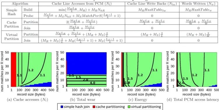
Comparisons of the Three Algorithms. Figure 5 com-pares the three algorithms analytically using the formulas in Table 4. We assumeRandS have the same record size, and it is a primary-foreign key join (thusM atchP erS= 1). From left to right, Figures 5(a) to (d) show the comparison results for four metrics: (a) cache accesses (Nl), (b) total

wear, (c) energy, and (d) total PCM access latency. In each figure, we vary the record size from 1 to 500 bytes, and the number of matches perR record (M atchP erR) from 1 to 50. Every point represents a configuration for the hash join. The color of a point shows the best scheme for the corre-sponding configuration: blue for simple hash join, red for cache partitioning, and green for virtual partitioning. For configurations where virtual partitioning is the best scheme, the contour lines show the relative benefits of virtual parti-tioning compared to the second best scheme.

Figure 5(a) focuses on CPU cache performance, which is the main consideration for previous cache-friendly hash join designs. We see that as expected, simple hash join is the best scheme when record size is very large and cache partition-ing is the best scheme when record size is small. Compared to simple hash join, virtual partitioning avoids the many cache misses caused by hash table accesses. Compared to

(7)

cache partitioning, virtual partitioning reduces the number of cache misses during the partition phase, while paying ex-tra cache misses for accessing scattered records in the join phase. As a result, virtual partitioning achieves the smallest number of cache misses for a large number of configurations in the middle between the red and blue points.

Figures 5(b) to (d) show the comparison results for the three PCM metrics. First of all, we see that the figures are significantly different from Figure 5(a). This means that introducing PCM main memory can significantly im-pact the relative benefits of the algorithms. Second, very few configurations benefit from cache partitioning because it incurs a large number of PCM writes in the partition phase, adversely impacting its PCM performance. Third, in Figure 5(b), virtual partitioning achieves the smallest num-ber of writes whenM atchP erR≤18. Virtual partitioning avoids many of the expensive PCM writes in the partition phase of the cache partitioning algorithm. Interestingly, simple hash join achieves the smallest number of writes when M atchP erR ≥ 19. This is because as M atchP erR increases, the number ofS records (MS) increases

propor-tionally, leading to a larger number of PCM writes for virtual partitioning, while the number of PCM writes in simple hash join is not affected. The cross-over point is 19 here. Finally, virtual partitioning presents a good balance between cache line accesses and PCM writes, and it excels in energy and total PCM access latency in most cases.

4. EXPERIMENTAL EVALUATION

We evaluate our proposed B+_{-tree and hash join}

algo-rithms through cycle-accurate simulations in this section. We start by describing the simulator used in the experi-ments. Then we present the experimental results for B+

-trees and hash joins. Finally, we perform sensitivity analysis for PCM parameters.

4.1 Simulation Platform

We extended a cycle-accurate out-of-order X86-64 sim-ulator, PTLsim [20], with PCM support. PTLsim is used extensively in computer architecture studies and is currently the only publicly available cycle-accurate simulator for out-of-order x86 micro-architectures. The simulator models the details of a superscalar out-of-order processor, including in-struction decoding, micro-code, branch prediction, function units, speculation, and a three-level cache hierarchy. PTL-sim has multiple use modes; we use PTLPTL-sim to PTL-simulate single 64-bit user-space applications in our experiments.

We extended PTLsim in the following ways to model PCM. First, we model data comparison writes for PCM writes. When writing a cache line to PCM, we compare the new line with the original line to compute the number of modi-fied bits and the number of modimodi-fied words. The former is used to compute PCM energy consumption, while the latter impacts PCM write latency. Second, we model four paral-lel PCM memory ranks. Accesses to different ranks can be carried out in parallel. Third, we model the details of cache line write back operations carefully. Previously, PTLsim as-sumes that cache line write backs can be hidden completely, and does not model the details of this operation. Because PCM write latency is significantly longer than its read la-tency, cache line write backs may actually keep the PCM busy for a sufficiently long time to stall front-end cache line fetches. Therefore, we implemented a 32-entry FIFO write

Table 5: Simulation Setup. Simulator PTLsim enhanced with PCM support Processor Out-of-order X86-64 core, 3GHz CPU

cache

Private L1D (32KB, 8-way, 4-cycle latency), private L2 (256KB, 8-way, 11-cycle latency), shared L3 (8MB, 16-way, 39-cycle latency), all caches with 64B lines,

64-entry DTLB, 32-entry write back queue PCM

4 ranks, read latency for a cache line: 230 cycles, write latency per 8B modified word: 450 cycles, Erb= 2 pJ,Ewb = 16 pJ

queue in the on-chip memory controller, which keeps track of dirty cache line evictions and performs the PCM writes asynchronously in the background.

Table 5 describes the simulation parameters. The cache hierarchy is modeled after the recent Intel Nehalem pro-cessors [14]. The PCM latency and energy parameters are based on a previous computer architecture study [15]. We adjusted the latency in cycles according to the 3GHz pro-cessor frequency and the DDR3 bus latency. The word size of 8 bytes per iteration of write operations is based on [8].

4.2 B

+

_{-Tree Index}

We implemented four variants of B+

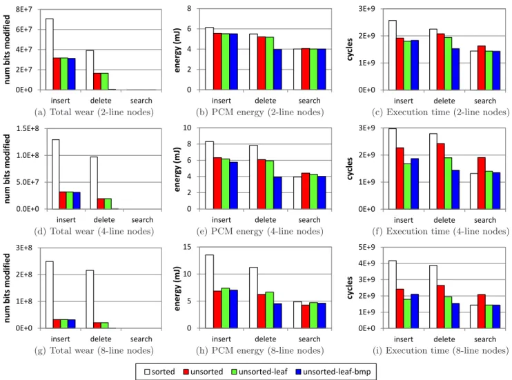
-trees as described in Section 3.2: sorted, unsorted, unsorted leaf, and unsorted leaf with bitmap. Figure 6 compares the four schemes for common index operations. In every experiment, we popu-late the trees with 50 million entries. An entry consists of an 8-byte integer key and an 8-byte pointer. We populate the nodes 75% full initially. We randomly shuffle the entries in all unsorted nodes so that the nodes represent the sta-ble situations after updates. Note that the total tree size is over 1GB, much larger than the largest CPU cache (8MB). For the insertion experiments, we insert 500 thousand ran-dom new entries into the trees back to back, and report total wear in number of PCM bits modified, PCM energy consumption in millijoules, and execution time in cycles for the entire operation. Similarly, we measure the performance of 500 thousand back-to-back deletions for the deletion ex-periments, and 500 thousand back-to-back searches for the search experiments. We vary the node size of the trees. As suggested by previous studies, the best tree node sizes are a few cache lines large [5, 12]. Since a one-line (64B) node can contain only 3 entries, which makes the tree very deep, we show results for node sizes of 2, 4, and 8 cache lines.

The sub-figures in Figure 6 are arranged as a 3x3 ma-trix. Every row corresponds to a node size. Every column corresponds to a performance metric. In every sub-figure, there are three groups of bars, corresponding to the inser-tion, deleinser-tion, and search experiments. The bars in each group show the performance of the four schemes. (Note that search does not incur any wear.) We observe the following points in Figure 6.

First, compared to the conventional sorted trees, all the three unsorted schemes achieve better total wear, energy consumption, and execution time for insertions and dele-tions, the two index operations that incur PCM writes. The sorted trees pay the cost of moving the sorted array of en-tries in a node to accommodate insertions and deletions. In contrast, the unsorted schemes all save PCM writes by al-lowing entries to be unsorted upon insertions and deletions. This saving increases as the node size increases. Therefore,

(8)

2E+7 4E+7 6E+7 8E+7 m b it s mo d ifi ed 0E+0 2E+7 4E+7 6E+7 8E+7

insert delete search

n u m b it s mo d ifi ed 0E+0 2E+7 4E+7 6E+7 8E+7

n u m b it s mo d ifi ed 8 0 2 4 6 8

e ne rg y (m J) 0 2 4 6 8

e ne rg y (m J) 3E+9 0E+0 1E+9 2E+9 3E+9

cycles

0E+0 1E+9 2E+9 3E+9

cycles

0E+0 1E+9 2E+9 3E+9

cycles

0E+0 1E+9 2E+9 3E+9

cycles

0E+0 1E+9 2E+9 3E+9

cycles

(a) Total wear (2-line nodes) (b) PCM energy (2-line nodes) (c) Execution time (2-line nodes)

5.0E+7 1.0E+8 1.5E+8 m b it s mo d ifi ed 0.0E+0 5.0E+7 1.0E+8 1.5E+8

n u m b it s mo d ifi ed 0.0E+0 5.0E+7 1.0E+8 1.5E+8

n u m b it s mo d ifi ed 10 0 2 4 6 8 10

e ne rg y (m J) 0 2 4 6 8 10

e ne rg y (m J) 3E+9 0E+0 1E+9 2E+9 3E+9

cycles

0E+0 1E+9 2E+9 3E+9

cycles

0E+0 1E+9 2E+9 3E+9

cycles

0E+0 1E+9 2E+9 3E+9

cycles

0E+0 1E+9 2E+9 3E+9

cycles

(d) Total wear (4-line nodes) (e) PCM energy (4-line nodes) (f) Execution time (4-line nodes)

1E+8 2E+8 3E+8 m b it s mo d ifi ed 0E+0 1E+8 2E+8 3E+8

n u m b it s mo d ifi ed 0E+0 1E+8 2E+8 3E+8

n u m b it s mo d ifi ed 15 0 5 10 15

e ne rg y (m J) 0 5 10 15

e ne rg y (m J) 4E+9 5E+9 0E+0 1E+9 2E+9 3E+9 4E+9 5E+9

cycles 0E+0 1E+9 2E+9 3E+9 4E+9 5E+9

cycles

(g) Total wear (8-line nodes) (h) PCM energy (8-line nodes) (i) Execution time (8-line nodes)

sorted unsorted unsortedͲleaf unsortedͲleafͲbmp

Figure 6: B+_{-tree performance. (50 million entries in trees; 75% full; “insert”: inserting 500 thousand}

random keys; “delete”: randomly deleting 500 thousand existing keys; “search”: searching for 500 thousand random keys)

the performance gaps widen as the node size grows from 2 cache lines to 8 cache lines.

Second, compared to the conventional sorted trees, the scheme with all nodes unsorted suffers from slower search time by a factor of 1.13–1.46X because the hot, top tree nodes stay in CPU cache, and a search incurs a lot of in-struction overhead in the unsorted non-leaf nodes. In con-trast, the two schemes with only unsorted leaf nodes achieve similar search time as the sorted scheme.

Third, comparing the two unsorted leaf schemes, we see that unsorted leaf with bitmap achieves better total wear, energy, and time for deletions. This is because unsorted leaf with bitmap often only needs to mark one bit in a leaf bitmap for a deletion (and the total wear is about 5E5 bits modified), while unsorted leaf has to overwrite the deleted entry with the last entry in a leaf node and update the counter in the node. On the other hand, the unsorted leaf with bitmap suffers from slightly higher insertion time be-cause of the instruction overhead of handling the bitmap and the holes in a leaf node.

Overall, we find that the two unsorted leaf schemes achieve the best performance. Compared to the conventional sorted B+

-tree, the unsorted leaf schemes improve total wear by

a factor of 7.7–436X, energy consumption by a factor of 1.7–2.5X, and execution time by a factor of 2.0–2.5X for insertions and deletions, while achieving similar search per-formance. If the index workload consists of mainly insertions and searches (with the tree size growing), we recommend the normal unsorted leaf. If the index workload contains a lot of insertions and a lot of deletions (e.g., the tree size stays roughly the same), we recommend the unsorted leaf scheme with bitmap.

4.3 Hash Joins

We implemented the three hash join algorithms as dis-cussed in Section 3.3: simple hash join, cache partitioning, and virtual partitioning. We model in-memory join opera-tions, where the input relationsRandS are in main mem-ory. The algorithms build in-memory hash tables on theR relation. To hash aR record, we compute an integer hash code from its join key field, and modulo this hash code by the size of the hash table to obtain the hash slot. Then we insert (hash code, pointer to the R record) into the hash slot. Conflicts are resolved through chained hashing. To probe anSrecord, we compute the hash code from its join key field, and use the hash code to look up the hash

(9)

ta-ϭнϴ ϭнϵ ŶƵŵ ďŝƚƐ ŵ ŽĚŝĨŝĞĚ ;ůŽŐ ƐĐĂůĞͿ ϭнϲ ϭнϳ ϭнϴ ϭнϵ ϮϬ ϰϬ ϲϬ ϴϬ ϭϬϬ ŶƵŵ ďŝƚƐ ŵ ŽĚŝĨŝĞĚ ;ůŽŐ ƐĐĂůĞͿ ƌĞĐŽƌĚƐŝǌĞ ϭнϲ ϭнϳ ϭнϴ ϭнϵ ϮϬ ϰϬ ϲϬ ϴϬ ϭϬϬ ŶƵŵ ďŝƚƐ ŵ ŽĚŝĨŝĞĚ ;ůŽŐ ƐĐĂůĞͿ ƌĞĐŽƌĚƐŝǌĞ ϭнϲ ϭнϳ ϭнϴ ϭнϵ ϮϬ ϰϬ ϲϬ ϴϬ ϭϬϬ ŶƵŵ ďŝƚƐ ŵ ŽĚŝĨŝĞĚ ;ůŽŐ ƐĐĂůĞͿ ƌĞĐŽƌĚƐŝǌĞ 30 40 J) 0 10 20 30 40 20B 40B 60B 80B 100B e ne rg y (m J) recordsize 4E+9 6E+9 8E+9 1E+10 cyc le s 0E+0 2E+9 4E+9 6E+9 8E+9 1E+10 20B 40B 60B 80B 100B cycles recordsize 0E+0 2E+9 4E+9 6E+9 8E+9 1E+10 20B 40B 60B 80B 100B cycles recordsize 0E+0 2E+9 4E+9 6E+9 8E+9 1E+10 20B 40B 60B 80B 100B cycles recordsize 0E+0 2E+9 4E+9 6E+9 8E+9 1E+10 20B 40B 60B 80B 100B cycles recordsize 0E+0 2E+9 4E+9 6E+9 8E+9 1E+10 20B 40B 60B 80B 100B cycles recordsize

(a) Total wear (b) PCM energy (c) Execution time

(2 matches per R record) (2 matches per R record) (2 matches per R record)

ŶƵŵ ďŝƚƐ ŵ ŽĚŝĨŝĞĚ ;ůŽŐ ƐĐĂůĞͿ ŶƵŵ ďŝƚƐ ŵ ŽĚŝĨŝĞĚ ;ůŽŐ ƐĐĂůĞͿ ŶƵŵŵĂƚĐŚĞƐƉĞƌZƌĞĐŽƌĚ ŶƵŵ ďŝƚƐ ŵ ŽĚŝĨŝĞĚ ;ůŽŐ ƐĐĂůĞͿ ŶƵŵŵĂƚĐŚĞƐƉĞƌZƌĞĐŽƌĚ ŶƵŵ ďŝƚƐ ŵ ŽĚŝĨŝĞĚ ;ůŽŐ ƐĐĂůĞͿ ŶƵŵŵĂƚĐŚĞƐƉĞƌZƌĞĐŽƌĚ 50 60 70 J) 0 10 20 30 40 50 60 70 1 2 4 6 8 e ne rg y (m J)

nummatchesperRrecord

2E+10 3E+10 cyc le s 0E+0 1E+10 2E+10 3E+10 1 2 4 6 8 cycles

nummatchesperRrecord 0E+0 1E+10 2E+10 3E+10 1 2 4 6 8 cycles

nummatchesperRrecord (d) Total wear (60B records) (e) PCM energy (60B records) (f) Execution time (60B records)

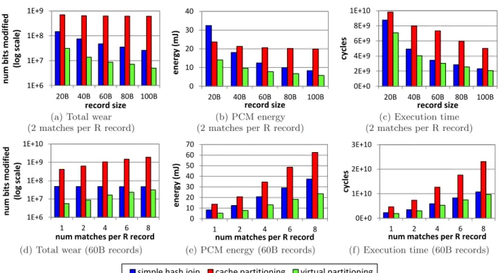
Figure 7: Hash join performance. (50MB R table joins S table, varying the record size from 20B to 100B and varying the number of matches per R record from 1 to 8.)

ble. When there is an entry with the matching hash code, we check the associatedRrecord to make sure that the join keys actually match. The join results are sent to a high-level operator that consumes the results. In our implementation, the high-level operator simply increments a counter.

Figure 7 compares the three hash join algorithms. The R relation is 50MB large. Both relations have the same record size. We vary the record size from 20B to 100B in Figures 7(a)–(c). We vary the number of matches per R record (M atchP erR) from 1 to 8 in Figures 7(d)–(f); in other words, the size ofS varies from 50MB to 400MB. We report total wear, energy consumption, and execution times for every set of experiments.

The results in Figure 7 confirm our analytical comparison in Section 3.3. First, cache partitioning performs poorly in almost all cases because it performs a large number of PCM writes in its partition phase. This results in much higher total wear, higher energy consumption, and longer execution time compared to the other two schemes.

Second, compared to simple hash join, when varying record size from 20B to 100B, virtual partitioning improves total wear by a factor of 4.7–5.2X, energy consumption by a factor of 2.3–1.4X, and execution time by a factor of 1.24–1.12X. When varyingM atchP erRfrom 1 to 8, virtual partitioning improves total wear by a factor of 8.6–1.5X, energy con-sumption by a factor of 1.61–1.59X, and execution time by a factor of 1.19–1.11X.

Overall, virtual partitioning achieves the best performance among the three schemes in all the experiments. Compared to cache partitioning, virtual partitioning avoids copying data in the partition phase by remembering record IDs per partition. Compared to simple hash join, virtual partition-ing avoids excessive cache misses due to hash table accesses. Therefore, virtual partitioning achieves good behaviors for both PCM writes and cache accesses. Note that the record

size andM atchP erRsettings in the experiments fall in the region where virtual partitioning wins in Figure 5. There-fore, the experimental results confirm our analytical com-parison in Section 3.3.

4.4 PCM Parameter Sensitivity Analysis

In this section, we vary the energy and latency parameters of PCM in the simulator, and study the impact of the pa-rameter changes on the performance of the B+

-tree and hash join algorithms. Note that we still assume data comparison writes for PCM write.

Figure 8 varies the energy consumed by writing a PCM bit (Ewb) from 2pJ to 64pJ. The default value of Ewb is

16pJ, and 2pJ is the same as the energy consumed by read-ing a PCM bit. From left to right, Figures 8(a)–(c) show the impact of varying Ewb on the energy consumptions of

B+_{-tree insertions, B}+_{-tree deletions, and hash joins. First,}

we see that asEwbgets smaller, the curves become flat; the

energy consumption is more and more dominated by the cache line fetches for reads and for data comparison writes. Second, asEwbgets larger, the curves increase upwards

be-cause the largerEwbcontributes significantly to the overall

energy consumption. Third, changing Ewb does not

quali-tatively change our previous conclusions. For B+_{-trees, the}

two unsorted leaf schemes are still better than sorted B+

-trees. Among the three hash join algorithms, virtual parti-tioning is still the best.

Figure 9 varies the latency of writing a word to PCM (Tw) from 230 cycles to 690 cycles. The defaultTw is 450

cycles, and 230 is the same latency as reading a cache line from PCM. From left to right, Figures 8(a)–(c) show the impact of varyingTwon the execution times of B+-tree

in-sertions, B+

-tree deletions, and hash joins. We see that as Twincreases, the performance gaps among different schemes

(10)

5 10 15 20 25 30 e ne rg y (m J) sorted unsortedͲleaf unsortedͲleafͲbmp 0 5 10 15 20 25 30 2 4 8 16 32 64 e ne rg y (m J) Ewb(pJ) sorted unsortedͲleaf unsortedͲleafͲbmp 0 5 10 15 20 25 30 2 4 8 16 32 64 e ne rg y (m J) Ewb(pJ) sorted unsortedͲleaf unsortedͲleafͲbmp 15 20 25 (m J) sorted unsortedͲleaf unsortedͲleafͲbmp 0 5 10 15 20 25 2 4 8 16 32 64 e ne rg y (m J) Ewb(pJ) sorted unsortedͲleaf unsortedͲleafͲbmp 20 30 40 50 60 e ne rg y (m J)

simplehashjoin cachepartitioning virtualpartitioning 0 10 20 30 40 50 60 2 4 8 16 32 64 e ne rg y (m J) Ewb(pJ)

(a) B+_{-tree insertions} _{(b) B}+_{-tree deletions} _{(c) Hash joins (2 matches per R record, 60B)}

Figure 8: Sensitivity analysis: varying energy consumed for writing a PCM bit (Ewb).

8 10 9 ) sorted unsortedͲleaf 0 2 4 6 8 10 230 450 690 cycles (x 1 e 9 ) Tw(cycles) sorted unsortedͲleaf unsortedͲleafbmp 0 2 4 6 8 10 230 450 690 cycles (x 1 e 9 ) Tw(cycles) sorted unsortedͲleaf unsortedͲleafbmp 0 2 4 6 8 10 230 450 690 cycles (x 1 e 9 ) Tw(cycles) sorted unsortedͲleaf unsortedͲleafbmp 0 2 4 6 8 10 230 450 690 cycles (x 1 e 9 ) Tw(cycles) sorted unsortedͲleaf unsortedͲleafbmp 8 10 9 ) sorted unsortedͲleaf 0 2 4 6 8 10 230 450 690 cycles (x 1 e 9 ) Tw(cycles) sorted unsortedͲleaf unsortedͲleafbmp 0 2 4 6 8 10 230 450 690 cycles (x 1 e 9 ) Tw(cycles) sorted unsortedͲleaf unsortedͲleafbmp 5 10 15 le s (x 1 e 9 )

simplehashjoin cachepartitioning virtualpartitioning 0 5 10 15 230 450 690 cycles (x 1 e 9 ) Tw(cycles) simplehashjoin cachepartitioning virtualpartitioning

(a) B+

-tree insertions (b) B+

-tree deletions (c) Hash joins (2 matches per R record, 60B) Figure 9: Sensitivity analysis: varying latency of writing a word to PCM (Tw).

join and virtual partitioning is 6% whenTw is 230 cycles.)

We find that previous conclusions still hold for B+

-trees and hash joins.

5. RELATED WORK

PCM Architecture. As discussed in previous sections, several recent studies from the computer architecture com-munity have proposed solutions to make PCM a replacement for or an addition to DRAM main memory. These studies address various issues including improving endurance [15, 21, 22, 32], improving write latency by reducing the number of PCM bits written [8, 15, 31, 32], preventing malicious wear-outs [26], and supporting error corrections [25]. How-ever, these studies focus on hardware design issues that are orthogonal to our focus on designing efficient algorithms for software running on PCM.

PCM-Based File Systems. BPFS [9], a file system de-signed for byte-addressable persistent memory, exploits both the byte-addressability and non-volatility of PCM. In addi-tion to being significantly faster than disk-based file sys-tems (even when they are run on DRAM), BPFS provides strong safety and consistency guarantees by using a new technique called short-circuit shadow paging. Unlike tradi-tional shadow paging file systems, BPFS uses copy-on-write at fine granularity to atomically commit small changes at any level of the file system tree. This avoids updates to the file system triggering a cascade of copy-on-write operations from the modified location up to the root of the file system tree. BPFS is a file system, and hence it does not consider the database algorithms we consider. Moreover, BPFS has been designed for the general class of byte-addressable per-sistent memory, and it does not consider PCM-specific issues such as read-write asymmetry or limited endurance. Battery-Backed DRAM. Battery-backed DRAM (BB-DRAM) has been studied as a byte-addressable, persistent memory. The Rio file cache [16] uses BBDRAM as the buffer cache, eliminating any need to flush dirty data to disk. The

Rio cache has also been integrated into databases as a per-sistent database buffer cache [18]. The Conquest file sys-tem [29] uses BBDRAM to store small files and metadata. eNVy [30] placed flash memory on the memory bus by us-ing a special controller equipped with a BBDRAM buffer to hide the block-addressable nature of flash. WAFL [13] keeps file system changes in a log in BBDRAM and only occasionally flushes them to disk. While BBDRAM may be an alternative to PCM, PCM has two main advantages over BBDRAM. First, BBDRAM is vulnerable to correlated failures; for example, the UPS battery will often fail ei-ther before or along with primary power, leaving no time to copy data out of DRAM. Second, PCM is expected to scale much better that DRAM, making it a better long-term option for persistent storage [3]. On the other hand, using PCM requires dealing with expensive writes and limited en-durance, a challenge not present with BBDRAM. Therefore, BBDRAM-based algorithms do not require addressing the challenges studied in this paper.

Main Memory Database Systems and Cache-Friendly Algorithms. Main memory database systems [11] maintain necessary data structures in DRAM and hence can exploit DRAM’s byte-addressable property. As discussed in Sec-tion 3.1, the tradiSec-tional design goals of main memory algo-rithms are low computation complexity and good CPU cache performance. Like BBDRAM-based systems, main mem-ory database systems do not need to address PCM-specific challenges. In this paper, we found that for PCM-friendly algorithms, one important design goal is to minimize PCM writes. Compared to previous cache-friendly B+_{-trees and}

hash joins, our new algorithms achieve significantly better performance in terms of PCM total wear, energy consump-tion, and execution time.

6. CONCLUSION

A promising non-volatile memory technology, PCM is ex-pected to play an important role in the memory hierarchy in the near future. This paper focuses on exploiting PCM

(11)

as main memory for database systems. Based on the unique characteristics of PCM (as opposed to DRAM and NAND flash), we identified the importance of reducing PCM writes for optimizing PCM endurance, energy, and performance. Specifically, we applied this observation to database algo-rithm design, and proposed new B+

-tree and hash join de-signs that significantly improve the state-of-the-art.

As future work in the PCM-DB project, we are interested in optimizing PCM writes for different aspects of database system designs, including important data structures, query processing algorithms, and transaction logging and recovery. The latter is important for achieving transaction atomicity and durability. BPFS proposed a different solution based on shadow copying and atomic writes [9]. It is interesting to compare this proposal with conventional database trans-action logging, given the goal of reducing PCM writes.

Moreover, another interesting aspect to study is the fine-grain non-volatility of PCM. Challenges may arise in hierar-chies where DRAM is explicitly controlled by software. Be-cause DRAM contents are lost upon restart, the relationship between DRAM and PCM must be managed carefully; for example, pointers to DRAM objects should not be stored in PCM. On the other hand, the fine-grain non-volatility may enable new features, such as “instant-reboot” that resumes the execution states of long-running queries upon crash re-covery so that useful work is not lost.

7. REFERENCES

[1] P. A. Boncz, S. Manegold, and M. L. Kersten. Database architecture optimized for the new bottleneck: Memory access. InVLDB, 1999. [2] L. Bouganim, B. J´onsson, and P. Bonnet. uFLIP:

Understanding flash IO patterns. InCIDR, 2009. [3] G. W. Burr, M. J. Breitwisch, M. Franceschini,

D. Garetto, K. Gopalakrishnan, B. Jackson, B. Kurdi, C. Lam, L. A. Lastras, A. Padilla, B. Rajendran, S. Raoux, and R. S. Shenoy. Phase change memory technology.J. Vacuum Science, 28(2), 2010. [4] S. Chen, A. Ailamaki, P. B. Gibbons, and T. C.

Mowry. Improving hash join performance through prefetching. InICDE, 2004.

[5] S. Chen, P. B. Gibbons, and T. C. Mowry. Improving index performance through prefetching. InSIGMOD, 2001.

[6] S. Chen, P. B. Gibbons, T. C. Mowry, and G. Valentin. Fractal prefetching B+

-trees: Optimizing both cache and disk performance. InSIGMOD, 2002. [7] S. Cho. Personal communication, 2010.

[8] S. Cho and H. Lee. Flip-N-Write: A simple deterministic technique to improve PRAM write performance, energy and endurance. InMICRO, 2009. [9] J. Condit, E. B. Nightingale, C. Frost, E. Ipek, B. C.

Lee, D. Burger, and D. Coetzee. Better I/O through byte-addressable, persistent memory. InSOSP, 2009. [10] E. Doller. Phase change memory and its impacts on

memory hierarchy. http://www.pdl.cmu.edu/SDI/ 2009/slides/Numonyx.pdf, 2009.

[11] H. Garcia-Molina and K. Salem. Main memory database systems: An overview.IEEE TKDE, 4(6), 1992.

[12] R. A. Hankins and J. M. Patel. Effect of node size on

the performance of cache-conscious B+-trees. In SIGMETRICS, 2003.

[13] D. Hitz, J. Lau, and M. Malcolm. File system design for an NFS file server appliance. InUSENIX Winter Technical Conference, 1994.

[14] Intel Corp. First the tick, now the tock: Intel

micro-architecture (Nehalem). http://www.intel.com/ technology/architecture-silicon/next-gen/319724.pdf. [15] B. C. Lee, E. Ipek, O. Mutlu, and D. Burger.

Architecting phase change memory as a scalable DRAM alternative. InISCA, 2009.

[16] D. E. Lowell and P. M. Chen. Free transactions with Rio Vista.Operating Systems Review, 31, 1997. [17] S. Nath and P. B. Gibbons. Online maintenance of

very large random samples on flash storage.The VLDB Journal, 19(1), 2010.

[18] W. T. Ng and P. M. Chen. Integrating reliable memory in databases.The VLDB Journal, 7(3), 1998. [19] PCM-DB.

http://www.pittsburgh.intel-research.net/projects/hi-spade/pcm-db/. [20] PTLsim. http://www.ptlsim.org/.

[21] M. K. Qureshi, J. P. Karidis, M. Franceschini, V. Srinivasan, L. Lastras, and B. Abali. Enhancing lifetime and security of PCM-based main memory with start-gap wear leveling. InMICRO, 2009. [22] M. K. Qureshi, V. Srinivasan, and J. A. Rivers.

Scalable high performance main memory system using phase-change memory technology. InISCA, 2009. [23] J. Rao and K. A. Ross. Making B+-trees cache

conscious in main memory. InSIGMOD, 2000. [24] Samsung. Samsung ships industry’s first multi-chip

package with a PRAM chip for handsets. http:// www.samsung.com/us/business/semiconductor/ newsView.do?news id=1149, April 2010.

[25] S. E. Schechter, G. H. Loh, K. Straus, and D. Burger. Use ECP, not ECC, for hard failures in resistive memories. InISCA, 2010.

[26] N. H. Seong, D. H. Woo, and H.-H. S. Lee. Security refresh: Prevent malicious wear-out and increase durability for phase-change memory with dynamically randomized address mapping. InISCA, 2010.

[27] A. Shatdal, C. Kant, and J. F. Naughton. Cache conscious algorithms for relational query processing. InVLDB, 1994.

[28] H.-W. Tseng, H.-L. Li, and C.-L. Yang. An energy-efficient virtual memory system with flash memory as the secondary storage. InInt’l Symp. on Low Power Electronics and Design (ISPLED), 2006. [29] A.-I. Wang, P. L. Reiher, G. J. Popek, and G. H.

Kuenning. Conquest: Better performance through a disk/persistent-RAM hybrid file system. InUSENIX Annual Technical Conference, 2002.

[30] M. Wu and W. Zwaenepoel. eNVy: a non-volatile, main memory storage system. InASPLOS, 1994. [31] B.-D. Yang, J.-E. Lee, J.-S. Kim, J. Cho, S.-Y. Lee,

and B.-G. Yu. A low power phase-change random access memory using a data-comparison write scheme. InIEEE ISCAS, 2007.

[32] P. Zhou, B. Zhao, J. Yang, and Y. Zhang. A durable and energy efficient main memory using phase change memory technology. InISCA, 2009.

Rethinking Database Algorithms for Phase Change Memory