Hybrid Three-Phase Load Flow Method for Ungrounded Distribution Systems

MITSUBISHI ELECTRIC RESEARCH LABORATORIES http://www.merl.com

Hybrid Three-Phase Load Flow Method for Ungrounded

Distribution Systems

Sun, H.; Nikovski, D.; Ohno, T.; Takano, T.; Kojima, Y. TR2012-082 October 2012

Abstract

This paper proposes a hybrid three-phase load flow method for ungrounded distribution systems. Based on topology connectivity analysis, the system is partitioned into a mainline system and multiple tap systems. A Newton method with constant admittance matrix is used to solve the mainline system, such that zero impedance branches are merged into adjacent impedance branches to be considered, and constant active-power and voltage-magnitude (PV) buses with three-phase balanced voltages are transformed into single- phase PV buses to be modeled. A backward/forward sweep with loop compensation is used to solve the tap systems, such that a transformer and a voltage regulator is modeled using line-to-line voltages, a distribution line is simplified as a series branch, and loop compensation current is initialized based on loop downstream loads and the impedances of loop paths. Test results of sample systems are given to demonstrate the effectiveness of the proposed method.

2012 IEEE PES Innovative Smart Grid Technologies Conference - Europe (ISGT Europe)

This work may not be copied or reproduced in whole or in part for any commercial purpose. Permission to copy in whole or in part without payment of fee is granted for nonprofit educational and research purposes provided that all such whole or partial copies include the following: a notice that such copying is by permission of Mitsubishi Electric Research Laboratories, Inc.; an acknowledgment of the authors and individual contributions to the work; and all applicable portions of the copyright notice. Copying, reproduction, or republishing for any other purpose shall require a license with payment of fee to Mitsubishi Electric Research Laboratories, Inc. All rights reserved.

Copyright cMitsubishi Electric Research Laboratories, Inc., 2012 201 Broadway, Cambridge, Massachusetts 02139

1

Abstract-- This paper proposes a hybrid three-phase load flow method for ungrounded distribution systems. Based on topology connectivity analysis, the system is partitioned into a mainline system and multiple tap systems. A Newton method with constant admittance matrix is used to solve the mainline system, such that zero impedance branches are merged into adjacent impedance branches to be considered, and constant active-power and voltage-magnitude (PV) buses with three-phase balanced voltages are transformed into single-phase PV buses to be modeled. A backward/forward sweep with loop compensation is used to solve the tap systems, such that a transformer and a voltage regulator is modeled using line-to-line voltages, a distribution line is simplified as a series branch, and loop compensation current is initialized based on loop downstream loads and the impedances of loop paths. Test results of sample systems are given to demonstrate the effectiveness of the proposed method.

Index Terms-- Distribution system; Three-phase; Load Flow; Ungrounded; Real-time.

I. INTRODUCTION

ITH the increasing deployment of smart grid technologies such as renewable energies, demand responses, pluggable electric vehicles and advanced network controllers, the operation of distribution systems becomes much more complicated and challenging than before. Computational tools suitable for real-time monitoring of large-scale distribution system are highly desired by the electric utilities for assisting their operators to ensure the safety, security and efficiency of the operation of distribution systems under fluctuating and less-predictable situations introduced by smart grid applications. As a fundamental tool of time monitoring, three-phase real-time load flow is playing an important role by analyzing the steady-state performance of distribution systems in a timely manner.

Various methods for solving three-phase power flow problems are known. Most of these methods are mainly designed for grounded distribution systems, and might not be

Hongbo Sun and Daniel Nikovski are with the Mitsubishi Electric Research Laboratories, Cambridge, MA 02139 USA (e-mail: [email protected]; [email protected]).

Tetsufumi Ohno, Tomihiro Takano, and Yasuhiro Kojima are with the Mitsubishi Electric Corporation, Hyogo 661-8661 Japan (e-mail: [email protected]; Takano.Tomihiro@df. MitsubishiElectric.co.jp; [email protected]).

applied to the ungrounded systems directly. These methods differ in both the form of the equations describing the system and in the numerical techniques used. Usually, either topology- or matrix-based methods are employed. Topology-based methods are suitable for radial systems, and include the Backward/Forward sweep method[1] and Ladder method[2]. Compensation schemes[1], [3]-[4] must be used when loops or PV buses are present in the system, and the existing schemes are less efficient when dealing with PV buses. The admittance-matrix based methods include the Implicit Z-bus method [5]-[6], the Newton-Raphson method [7]-[8], the Fast Decoupled method [9], and the Sequence Decoupling method [10]-[11]. All of these methods have their own limitations when applied to large systems, either in terms of modeling capabilities, or in terms of computational efficiency.

This paper proposes a new hybrid three-phase load flow method that is suitable for real-time applications in large-scale ungrounded distribution systems. Based on topology connectivity analysis, the distribution system is partitioned into a mainline system and multiple tap systems to be solved by means of a Newton method with constant Jacobian matrix, and a backward/forward sweep method with loop compensation, respectively. The impact of zero-impedance branches such as voltage regulators have been modeled by merging those branches with adjacent impedance branches, such that the inaccuracy or divergence problems introduced by adding small impedances into those branches, that is commonly used by conventional methods, can been avoided. Unlike the common practice to set active power for each phase arbitrarily, the proposed method models the control requirements for constant active-power and voltage-magnitude (PV) buses with three-phase balanced voltages precisely, that is, by maintaining the sum of three-phase active power constant, and by maintaining three-phase voltages balanced and with constant magnitudes. Instead of initializing the bus voltages with the setting of the swing bus, and loop compensation currents as zeros, the method sets the initial bus voltages based on the swing-bus voltage and the amplifier factors of transformers and regulators along paths connecting each bus with the swing bus, and initializes the loop compensation currents based on the connected loop loads and an allocation factor matrix defined solely by the loop path impedances. The method used a closed-form formula to uniquely convert line-to-line voltages into phase-to-ground

Hybrid Three-Phase Load Flow Method for

Ungrounded Distribution Systems

Hongbo Sun,

Senior Member, IEEE

, Daniel Nikovski,

Member, IEEE

, Tetsufumi Ohno, Tomihiro

Takano, and Yasuhiro Kojima,

Member, IEEE

ungrounded transformers in tap systems are solved by using admittance models based on line-to-line voltages in order to avoid the resulting matrix singularity when using models based on phase-to-ground voltage. The formula also enables the construction of the nodal admittance matrix of the mainline system, based on amplifying factors of zero-impedance branches written in line-to-line voltages. The solution process for a tap system is further simplified by integrating line charging into connected buses, and only series line currents are used during iterations.

II. THE PROPOSED METHOD

A. System Partitioning

Based on the topology analysis, the proposed method has partitioned the distribution system into a mainline system and a set of tap systems. The mainline system is formed by mainline buses connecting a swing bus to a set of PV buses, and the tap system is formed by one or more tap buses, such that the root bus of each tap system corresponds to a mainline bus.

Fig. 1 Distribution system partitioning

Fig. 1 shows an example of the partitioning of a distribution system into a corresponding mainline system and two tap systems 1 and 2. In the example, the mainline system includes five buses, including one swing bus m1, one PV bus

m2, and two root buses, t1 and t2 for two tap systems, 1 and 2. The mainline system is a radial system. Tap system 1 starts from a mainline bus t1, which is its root bus, and includes all buses and devices downstream to the bus t1. As can be seen, tap system 1 forms a loop. Tap system 2 starts from a corresponding root bus t2 of the mainline system, and includes all buses and devices downstream to bus t2. Tap system 2 has no loops and is a radial system.

Based on the number of devices connected between the study bus and the root, the tap systems can be divided into layers. For example, in Fig. 1, tap system 1 is divided into four layers, where the first layer contains one bus, and the last layer constants three buses. Similarly, tap system 2 is divided into three layers.

The power flows of distribution system is solving through iterative solving of the mainline system and tap systems, and a final solution is obtained when the required accuracy for the bus voltage or power mismatch is satisfied.

The mainline system is formed by mainline buses that reside on the paths between the swing bus and PV buses. The mainline system may be radial, or meshed. The modeled bus and phases in the mainline system are converted to nodes to construct the power flow equations. The number of nodes for each bus is equal to the number of modeled or available phases at the bus.

The power flow equations are formulated in polar coordinates and solved by Newton's method with a constant Jacobian matrix. The impacts of zero-impedance branches and voltage balance requirements of three-phase PV buses are embedded into the nodal admittance matrix of the mainline system.

1) Zero-impedance Branches

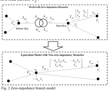
Many branches in a distribution system can be regarded as zero-impedance branches, such as step voltage regulators, switches, jumpers and very short lines. Usually, the impedances of those branches are very small and can be ignored. However, the consequence is that some entries in the resultant nodal admittance matrix become infinite, and thus the admittance matrix based approaches are inapplicable. In order to use admittance matrix based approaches, conventional methods have arbitrarily assigned small non-zero impedances to those branches. However, assigning such small impedances makes the analysis ill-conditioned, and load flow analysis is difficult to converge. In the proposed method, a different method is used that merges those zero-impedance branches with adjacent impedance branches into new non-zero impedance branches.

Fig. 2 gives an example of a generalized three-phase zero-impedance branch between bus m and bus p. One of the buses, for example the bus m, is assigned to be a master bus, and the other bus p is assigned to be a slave bus. The buses are connected by an ideal transformer. The slave bus is connected with a load current

I

_p.

Fig. 2 Zero-impedance branch model

The phase-to-ground voltages of its two terminal buses, and two directional phase currents on the branch are related to each other with the voltage amplifying factor matrices,

mp

V

3 and

pm

V

A

, and current amplifying factor matrices,

mp I

A

and pm I

A

as: pm I mp

A

I

I

mp

=

(1) mp I pm

A

I

I

pm

=

(2) p V m

A

V

V

mp

=

(3) m V p

A

V

V

pm

=

(4) where

I

_mpand

I

_pmare the vector of phase currents flowing from bus m to bus p, and bus p to bus m respectively,

m

V

and

V

_pare the vector of phase-to-ground voltages of bus m

and bus p. These amplifying factor matrices are determined according to the winding connection and tap positions for a transformer or a voltage regulator, and the phase connection for a switch, a short line or a jumper.

As shown in Fig.2, the zero-impedance branch is merged into adjacent impedance branches, such that the slave bus is not considered in the analysis of the model. In the example, the zero-impedance branch is connected to two branches by the slave bus p, and to another two branches by the master bus

m. Taking one adjacent branch between slave bus p and bus s

as an example, the relationship between the branch currents and the terminal bus voltages can be described as:

⎥

⎦

⎤

⎢

⎣

⎡

⎥

⎦

⎤

⎢

⎣

⎡

=

⎥

⎦

⎤

⎢

⎣

⎡

s p ss sp ps pp sp ps

V

V

Y

Y

Y

Y

I

I

(5) where,

I

_ps and

I

_spare the vector of phase branch currents flowing from bus p to s, and bus s to p,

V

_sis the vector of phase-to-ground voltages at bus s,

Y

ppand

Y

ss are the self

admittance matrices of bus p and s,

Y

psand

Y

spare the mutual

admittance between p and s, and s and p respectively. In the equivalent model, the zero-impedance branch and the slave bus p are removed. There are no changes for the branches connected to the master bus m. The branches connected to the slave bus p are reconnected to bus m, and the branch admittance matrices and the current injections at the master bus m are modified accordingly. The load current

I

_pat bus p

is modeled as an equivalent current at bus m, as

A

_I

I

_p mp

−

.

The branch between bus p and bus s is replaced with a new branch directly between bus m and bus s, and the branch currents,

I

_ms and

I

_sm, and the nodal voltages,

V

_m and

V

_s, are related as:

⎥

⎦

⎤

⎢

⎣

⎡

⎥

⎥

⎦

⎤

⎢

⎢

⎣

⎡

−

−

=

⎥

⎦

⎤

⎢

⎣

⎡

s m ss V sp ps I V pp I sm ms

V

V

Y

A

Y

Y

A

A

Y

A

I

I

pm mp pm mp (6) If the amplifying matrices are expressed with line-to-line voltages, (6) is replaced by the following equation:

⎥

⎦

⎤

⎢

⎣

⎡

⎥

⎥

⎦

⎤

⎢

⎢

⎣

⎡

₋

₋

=

⎥

⎦

⎤

⎢

⎣

⎡

s m ss LP V LL V PL V sp ps I LP V LL V PL V pp I sm ms

V

V

Y

C

A

C

Y

Y

A

C

A

C

Y

A

I

I

pm mp pm mp (7) where, _VLL mp

A

and _VLL pm

A

are the voltage amplifying factor matrices for the branch between bus m to bus p written in terms of line-to-line voltages, and line-to-line voltages at bus

m, and bus p,

V

_mLLand

V

_pLL are related as:

LL p LL V LL m

A

V

V

=

_mp (8) LL m LL V LL p

A

V

V

pm

=

(9) where,

C

_VLP is a conversion factor matrix to be used to convert voltages from phase-to-ground form into line-to-line one. Taken bus p as example, we have

p LP V LL p

C

V

V

=

(10) The matrix

C

_VLPis defined as:

⎥

⎥

⎥

⎦

⎤

⎢

⎢

⎢

⎣

⎡

−

−

−

=

1

0

1

1

1

0

0

1

1

LP V

C

(11) PL V

C

is a conversion factor matrix to be used to convert voltages in the form of line-to-line into phase-to-ground. For bus p, we have: LL p PL V p

C

V

V

=

(12) The conversion from line-to-line voltages into phase-to-ground voltages is not trivial. Due to unknown neutral-to-ground voltages, multiple results may be obtained based on the same line-to-line voltages. A conversion equation defined below is used to uniquely convert the line-to-line voltages to the phase-to-ground voltages:

⎥

⎥

⎥

⎦

⎤

⎢

⎢

⎢

⎣

⎡

−

−

−

=

3

/

1

3

1

0

0

3

1

3

/

1

3

1

0

3

1

PL V

C

(13)

The conversion is accurate when the voltages only include positive and negative sequence components, and is a good approximation if the zero-sequence components are small enough.

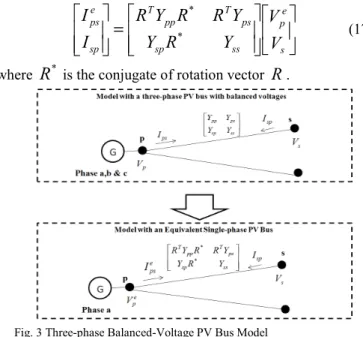
2) Three-phase PV buses with balanced voltages

A PV bus in the mainline system can be modeled as three PV nodes, if the power and voltage magnitude of each phase is regulated independently. However, if the bus is connected to a balanced voltage generation source, and the generator is regulated as constant voltage magnitude and constant total active power of three phases, accordingly, the three-phases of such bus have to be combined together to be modeled in the admittance matrix based power flow equations.

Assumed bus p is a PV bus with three-phase balanced voltages, its three phases a, b, and c can be combined into an equivalent single-phase e to be modeled. The equivalent phase

e can be any phase, and taken phase a as example, we can have: a p e p

V

V

=

(14) ps T e ps

R

I

I

₌

(15)

equivalent phase e, and phase a of bus p respectively, and

e ps

I

is the equivalent phase current flowing on the branch from bus p to bus s,

R

is a rotation vector to rotate all phases to the selected equivalence phase e,

R

T is the transpose of vector

R

. Assumed the equivalent phase is phase a, the rotation vector is defined as:

⎥

⎥

⎥

⎦

⎤

⎢

⎢

⎢

⎣

⎡

=

− o o j j

e

e

R

120 120

1

(16) Fig. 3 shows an example of determining an equivalent model for a distribution system with three-phase ganged regulated PV buses. In Fig. 3, the three phase PV bus p is connected to two branches. In the equivalent model, the three phases of PV buses with balanced voltages are combined into one single phase, and taking one branch between bus p and bus s as an example, the new branch model can be described as:

⎥

⎦

⎤

⎢

⎣

⎡

⎥

⎥

⎦

⎤

⎢

⎢

⎣

⎡

=

⎥

⎥

⎦

⎤

⎢

⎢

⎣

⎡

s e p ss sp ps T pp T sp e ps

V

V

Y

R

Y

Y

R

R

Y

R

I

I

* * (17) where

R

* is the conjugate of rotation vector

R

.

Fig. 3 Three-phase Balanced-Voltage PV Bus Model

3) Initial Bus Voltages

The Jacobian matrix is determined from the initial voltage setting. The initial voltages are set to the values at the swing bus multiplied with the aggregated voltage amplifying factor matrix introduced by the transformers or voltage regulators along the shortest path between the swing bus and the bus:

swing st

V p

A

V

V

(0)

=

∏

_{st (18)}

where,

V

_p(0) is the vector of initial voltages of bus p,

V

_swing is the voltage of the swing bus,

st

V

A

is the voltage amplifying factor matrix of a voltage regulator or transformer between two buses, bus s and bus t residing on the shortest path from the swing bus to the bus under consideration.

iteratively solving the following power mismatch equations:

[ ]

⎥

⎦

⎤

⎢

⎣

⎡

Δ

Δ

=

⎥

⎦

⎤

⎢

⎣

⎡

Δ

Δ

V

J

Q

P

θ

(19) where

_Δ

P

and

Δ

Q

are vectors of nodal power mismatches between the scheduled values and calculated values,

Δ

θ

and

V

Δ

are the vectors of node phase angle and voltage magnitude changes, and

J

are the Jacobian matrices of node active and reactive powers with respect to node phase angles and node voltage magnitudes. The Jacobian matrix is determined from the initial voltage setting, and factorized by using sparse LU decomposition or sparse Cholesky decomposition techniques, dependent on whether the matrix is symmetrical.

Any bus in the mainline system, which is not a PV, or swing bus, is treated as a PQ bus. Its equivalent phase powers are determined by the connected loads, capacitors, adjacent line charging, and downstream branches, if it is a root bus for a tap system. The equivalent power

S

x_p for bus p at phase x is determined according to:

*

)

(

∑

∈

+

=

p Tap s x ps x p x p x p

V

I

I

S

x

∈

{

a

,

b

,

c

}

(20)

where,

I

_px is the equivalent phase current of bus p at phase x,

x ps

I

is the equivalent phase current flowing through bus p

toward bus s at phase x,

Tap

_pis the set of buses that connect with bus p and reside in the tap system fed by the bus p.

C. The tap systems

A tap system is formed by a set of tap buses and the root bus of each tap system corresponds to a mainline bus. A backward/forward sweep scheme based on current summation with loop breakpoint compensation is applied.

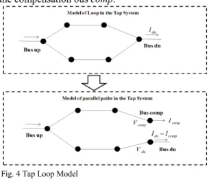
1) Loop Breakpoint Compensations

The loops in a tap system are broken into radial paths to be considered, and the downstream load current fed by the loop is allocated appropriately between two breakpoints, in order to maintain their voltages identical.

Fig. 4 shows an example construction of an equivalent model for a tap system having a loop formed between an upstream bus up and a downstream intersection bus dn. There are two paths available from the bus up to the bus dn. By replacing the downstream intersection bus with two breakpoints, i.e., one is the original bus dn, and the other is a new compensation bus comp, the loop is broken into two radial paths. Compensation current

I

_comp is added as a load to the compensation bus comp, and as a negative load to the original bus dn. In the proposed method, the compensation current

I

_comp is initially determined according to:

dn comp comp

A

I

5 where,

A

_comp is the allocation factor matrix to be used to

allocate downstream currents between two parallel loop paths. The allocation factor matrix is calculated based on the series impedance matrices of two paths according to:

1

)

(

− − − −

+

=

up dn up dn up comp comp

Z

Z

Z

A

(22) where,

Z

_up−dnis the impedance matrices for the path from the upstream bus up to the downstream bus dn, and

Z

_up−compis the impedance matrices for the path from the upstream bus up

to the compensation bus comp.

Fig. 4 Tap Loop Model

Using above equation, the loads at a downstream bus is initially allocated into two parallel paths. The currents along the two paths have to be adjusted, if the voltages at the two breakpoints are not identical. The incremental compensation current,

Δ

I

_comp is determined according to

comp comp comp

Z

V

I

=

Δ

Δ

−1 ₍₂₃₎ where,

Δ

V

_comp is the vector of the voltage difference between the compensation bus and the loop downstream intersection bus, and it can be calculated according to:

)

(

_{comp dn}

comp

V

V

V

=

−

Δ

(24)

where,

V

_comp and

V

dn are the phase-to-ground voltages at the

bus comp, and the bus dn, respectively.

Z

_comp is a loop impedance matrix, which for an independent loop can be determined as the sum of two path impedance matrices according to:

)

(

_{up dn up comp}

comp

Z

Z

Z

=

₋

+

_{− (25)}

If some of the loops share common paths between different loops, above equations can still be used to calculate the incremental compensation current, but the vector

Δ

I

_comp and

comp

V

Δ

includes the corresponding compensation current and voltage changes for each loop, and the loop impedance matrices

Z

_comp are formed based on the path impedance matrix for each loop, and common path impedance between loops.

2) Three-phase transformer branches

For a three-phase transformer, the backward/forward sweep steps need to calculate the inverse of its admittance matrices, and unfortunately for ungrounded connections, some of those matrices are singular. So, the line-to-line voltages, and phase currents are used to express the transformer model in tap systems. Because the primary and secondary buses are ungrounded, the sum of the three phase currents are zero, so only two phase currents are needed. And, only two of the three line-to-line voltages are needed as well. As an example, if we take currents at phase a and b as current variables, and line-to-line voltage between phase a to phase b, and phase b to phase c as voltage variables, the admittance model for a transformer between bus p and bus s are calculated according to: ' PL V mn LL mn

Y

C

Y

=

m

,

n

∈

{

p

,

s

}

(26) where,

C

_VPL' is a conversion matrix that used to calculate the phase-to-ground voltages for three phases based on line-to-line voltages between phase a to b, and b to c. The matrix is defined as:

⎥

⎥

⎥

⎦

⎤

⎢

⎢

⎢

⎣

⎡

−

−

−

=

3

/

2

3

/

1

3

/

1

3

/

1

3

/

1

3

/

2

' PL V

C

(27)

3) Three-phase line branches

In order to simplify the calculations for three-phase lines, the conventional π-model of distribution line is replaced with a series impedance branch by merging the line charging of shunt admittances into terminal buses as shown in Fig. 5.

Fig. 5 Tap Line Branch Model

Fig. 5 shows a model of distribution line connects bus p

and bus s. In the model, there is one series branch with impedance matrix,

Z

_psseand two shunt branches and each with half of shunt admittance matrix

Y

_pssh. Instead of solving the actual branch currents

I

'_ps and

I

_sp' directly, the proposed method has used the internal currents,

I

_ps and

I

_sp, that flow through the series impedances as the variables of the model to be solved. The actual branch currents can be determined by adding the line-charging currents to the internal currents, after the converged power flow solutions are obtained. By doing so, the computation efforts required for both backward sweep and forward sweep are significantly reduced. For example, for a backward sweep, the currents entering the line through the sending side p, can be directly set as negative of currents

4) Solving power flows of the tap systems

The power flows of a tap system is solved by using the backward/forward sweep scheme. The scheme includes two integrated steps. The first is the backward sweep step, or current summation step, which calculates the branch currents, starting from the branches at the last layers and moving towards the branches connected to the root bus. The second is the forward sweep step, or voltage update step, which updates the branch terminal voltages, starting from the branches in the first layer towards those in the last, and for each branch between a sending bus and a receiving bus, the voltage at the receiving bus is calculated using the updated voltages at the sending bus.

In a backward sweep, for any branch between sending bus p

and receiving bus s, the branch current entering the receiving bus s is determined according to:

∑

∈

−

−

=

s DN t x st x s x sp

I

I

I

x

∈

{

a

,

b

,

c

}

(28) where,

I

_sx is the equivalent current for bus s at phase x;

DN

_s is a set of downstream buses connected to the bus s, and

I

_stx is the phase current entering from bus s to a branch between bus

s and bus t.

The equivalent phase current for a bus takes contributions from the connected loads, capacitors, the line charging from connected lines, and the loop compensation currents, if it is a loop breakpoint. The loads and capacitors are Delta connected in an ungrounded system. The loads include constant power loads, constant current loads, and constant impedance loads. The equivalent phase currents at bus p,

I

_pcan be determined according to: comp s p sh ps LL p PL I p

C

I

Y

V

I

I

=

−

∑

(

)

+

2

1

(29) The first component of the right-hand side of (29) is the contribution from connected loads and capacitors which are calculated as line-to-line currents,

I

_pLL and then converted to phase currents using the current conversion factor matrix

C

_IPL

defined as:

⎥

⎥

⎥

⎦

⎤

⎢

⎢

⎢

⎣

⎡

−

−

−

=

1

1

0

0

1

1

1

0

1

PL I

C

(30)

The second component of the right-hand side of (29) is the contribution of line charging for all lines that connect to bus p, and

Y

_pssh is the shunt admittance of the line between bus p and

s. The third component,

I

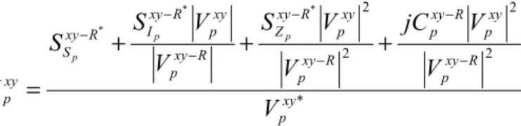
comp, is the contribution of loop compensation currents that can be determined using (21) and (23) if bus p is one of loop breakpoints, and is a positive value for the breakpoint corresponding to the compensation bus, and negative value for another breakpoint of the loop that corresponds to the original bus. The line-to-line current at bus

p between phase x and y is determined as follows:

* 2 2 xy p R xy p R xy p R xy p S xy p

V

V

V

V

S

I

p

+

−

+

₋

+

₋

=

}

,

,

{

ab

bc

ca

xy

∈

(31) where, _Sxy R p

S

− _, xy R Ip

S

− _and xy R Zp

S

− _{are the rated complex powers} at bus p and between phase x to phase y of constant power loads, constant current loads and constant impedance loads respectively;

C

_pxy−R _{is the rated reactive power generated at} bus p and phase x to y by connected capacitors; and

V

pxy−Ris

the rated voltage at bus p and between phase x to y.

In a forward sweep, the line-to-line voltages are used for calculation of transformers and voltage regulators, and then converted into phase-to-ground voltages by using the voltage conversion matrices. The phase-to-ground voltages are used for calculation of lines, and then converted into line-to-line voltages if the connected device is a transformer or voltage regulator.

III. NUMERICAL EXAMPLES

The proposed method was tested against several ungrounded distribution systems including the IEEE 37 node test feeder, and a 2000-node sample system. The testing was performed on a desktop computer with an Intel Core i7-960 processor. The maximum allowed power mismatch is set to be

5

10− _{per unit.}

A. Test results for the IEEE 37 node test feeder

Table I lists the test scenarios that are generated based on the IEEE 37 node test feeder in which scenario I is a pure radial system, scenario II is a looped system, scenario III is a radial system, but with additional distribution generation that is regulated as a PV bus, and scenario IV is a looped system with additional PV regulated generation.

TABLEI

TEST CASES BASED ON IEEE37 NODE TEST FEEDER

Test Scenarios

Configurations Characteristics of system

I Same as IEEE 37 node test feeder Radial system II Add two new branches to scenario

I, one between node 718 and 725, and one between node 729 and 732

System with two loops III Add one new node 788 with

three-phase PV regulation, and one branch between 711 and 788 to scenario I

Radial system with 1 PV bus

IV Add one new PV bus 788, and three new branches, between 788 and 711, 729 and 732, and 718 and 725 to scenario I

System with 2 loops and 1 PV bus

The computational performance of the proposed algorithm on those test scenarios is presented in Table II. The computational procedure includes two stages, the first stage involves the construction of connected islands based on the current or study-mode switch status through topology analysis, and the second stage involves the calculation of load flows for

7 each island that was constructed during the first stage. For

real-time applications, the first stage only needs to be re-executed when there are switching operations taking place in the system.

TABLEII

COMPUTATIONAL PERFORMANCES OF TEST CASES

Test Scenarios

CPU Time(ms)

Topology Analysis Load Flow Calculation

I 0.122 0.302

II 0.136 0.442

III 0.126 4.862

IV 0.172 5.890

As shown in Table I and II, the proposed algorithm is capable of analyzing three-phase load flows for ungrounded distribution systems with various configurations.

Tables III and IV list the computational results for test scenario III with different PV bus models, including three-phase independent regulating model, and three-three-phase ganged regulating model. The generation outputs of distributed generation and the swing bus are heavily dependent on the PV bus models to be used, and different models results in different generation dispatch results. It is obvious that if a three-phase ganged regulated PV bus were modeled as a three-phase independent regulated bus, the resultant power flow results might be wrong or at least not very inaccurate.

TABLEIII

PV BUS MODELS OF SCENARIO III PV Model Regulation Active Power Generations Magnitude of Phase-to-ground Voltage Three-phase Independent Regulated

The output of each phase is 100 kW

1.0 p.u for each phase

Three-phase Ganged Regulated

The total output of three phases is 300 kW

1.0 p.u. for each phase, and phase a leads 120 degree to phase b, and lags 120 degree to phase c TABLEIV

RESULTS FOR SCENARIO III WITH DIFFERENT PV MODELS

PV Model

PV Bus Swing Bus

Line-to-line Voltage Generation Output Generation Output Mag. (p.u) Angle (Deg.) kW kVar kW kVar Three-phase Independent Regulated 0.986 1.014 1.000 27.6 -92.4 146.3 100.0 100.0 100.0 489.1 320.5 440.4 728.8 637.0 858.8 79.5 -92.4 -132.7 Three-phase Ganged Regulated 1.000 1.000 1.000 27.2 -92.8 147.2 183.7 23.0 93.3 464.3 470.0 328.4 692.3 664.5 851.5 100.8 -99.5 851.5

B. Test results for the 2000-node sample system

The proposed method was also tested against a sample ungrounded distribution system with 2000 three-phase nodes. The sample system is a radial system, and has one substation and six feeders.

Similarly, four different test scenarios were generated based on the configuration of the 2000-node system. Scenario I is a pure radial system which uses the original configuration of the 2000-node system. Scenario II is a looped system which created by adding 12 loops to Scenario I. Scenario III is a

radial system, but with additional constant voltage sources by adding 3 PV buses into Scenario I. Scenario IV is a looped system with PV buses which created by adding 12 loops and 3 PV buses into Scenario I. The PV buses are located at the tails of associated feeders.

The testing results on the sample system and computation performance compared with other existing methods are provided in Table V. Three different algorithms have been compared, including the proposed method, the Gauss-Seidel method, and the Newton-Raphson method.

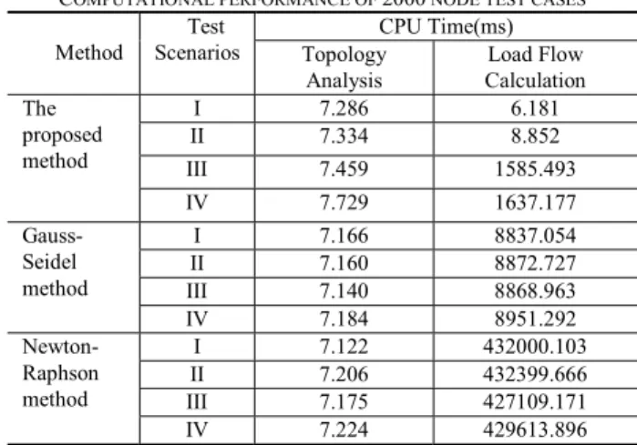
TABLEV

COMPUTATIONAL PERFORMANCE OF 2000 NODE TEST CASES

Method Test Scenarios CPU Time(ms) Topology Analysis Load Flow Calculation The proposed method I 7.286 6.181 II 7.334 8.852 III 7.459 1585.493 IV 7.729 1637.177 Gauss-Seidel method I 7.166 8837.054 II 7.160 8872.727 III 7.140 8868.963 IV 7.184 8951.292 Newton-Raphson method I 7.122 432000.103 II 7.206 432399.666 III 7.175 427109.171 IV 7.224 429613.896 From these test results, we can see that the proposed method is much more efficient than the Gauss-Seidel and Newton-Raphson algorithms when dealing with systems in radial configuration, or with limited number of loops and constant voltage sources. Taking Case IV as an example, it took 1637 ms for the proposed algorithm to find the final solution with the required precision. In comparison, it took 8951 ms for the Gauss-Seidel algorithm, and 429613 ms for the Newton-Raphson algorithm to find the solution with the same precision. Similar results can be found for the other three cases.

The test on the 2000 node system with radial topology showed that the proposed algorithm could find a solution within 7 ms, after the connectivity of the system was analyzed at the initial phase within 8 ms. In addition, the algorithm could also perform well for systems with arbitrary topology, including loops, at a slower speed. When 12 loops were added to the same 2000-node distribution system, calculation time was only slightly longer, 9 ms. Even with worst cases that generation sources are located far apart, ones at feeder heads, and the others at feeder tails as in the last two scenarios of table V, calculation time was considerably slower, but still within 2 seconds. Considering the size of test systems, and the platform that was used for testing, the calculation time is quite reasonable. Based on the preliminary results, it is safe to say that the proposed algorithm is suitable of real-time load flow analysis of large-scale ungrounded distribution systems.

IV.CONCLUSION

A new hybrid method for three-phase power flow analysis of ungrounded distribution systems was proposed, in which the topology of the distribution system is partitioned into a

system is formed by mainline buses connecting a swing bus and a set of constant voltage source buses, and the tap system is formed by one or many tap buses, such that a root bus of each tap system corresponds to a mainline bus.

The mainline system is solved by means of a Newton method with constant Jacobian matrix, in which the zero-impedance branches are merged into adjacent zero-impedance branches, and the three phases of balanced-voltage PV buses are merged into one single phase of PV buses. The tap systems are solved by a backward/forward sweep scheme with loop compensation, in which line-to-line voltage based voltage regulator and transformer parameters are used, and both line models and the calculation of initial loop compensation currents are simplified to speed up the solution procedure.

The numerical examples on sample systems have demonstrated the effectiveness of the proposed method and the suitableness of real time applications.

IV. REFERENCES

[1] D. Shirmohammadi, H. W. Hong, A. Semlyen, and G. X. Luo, “A Compensation-based Power Flow Method for Weakly Meshed Distribution and Transmission Networks,” IEEE Transactions on Power Systems, vol. 3, no.2, pp. 753-762, May 1988.

[2] W. H. Kersting: “A method to Teach the design and operation of a distribution system,” IEEE Transactions on Power Apparatus and Systems, vol. PAS-103, no.7, pp. 1945-1952, Jul. 1984.

[3] G.X. Luo and A. Semlyen, “Efficient Load Flow for Large Weakly Meshed Networks," IEEE Transactions on Power Systems, vol. 5, no. 4, pp. 1309-1316, Nov. 1990.

[4] W.C. Wu, and B.M. Zhang, “A three-phase power flow algorithm for distribution system power flow based on loop-analysis method,” Electrical Power and Energy Systems, vol. 30, pp. 8–15, Jun. 2008. [5] T.-H. Chen, M.-S. Chen, K.-J. Hwang, P. Kotas, and E.A. Chebli,

"Distribution system power flow analysis-a rigid approach," IEEE Transactions on Power Delivery, vol.6, no.3, pp.1146-1152, Jul 1991. [6] J. H. Teng, "A Modified Gauss-Seidel algorithm of three–phase power

flow analysis in distribution network," Electrical Power and Energy Systems, vol. 24, no. 2, pp. 97-102, Feb. 2002.

[7] V.M. da Costa, N. Martins, and J.L.R. Pereira, "Developments in the Newton Raphson power flow formulation based on current injections," IEEE Transactions on Power Systems, vol.14, no.4, pp.1320-1326, Nov 1999.

[8] P.A.N. Garcia, J.L.R. Pereira, S. Carneiro Jr.; V.M. da Costa, and N. Martins, "Three-phase power flow calculations using the current injection method," IEEE Transactions on Power Systems, vol.15, no.2, pp.508-514, May 2000.

[9] Whei-Min Lin, Jen-Hao Teng; “Three-phase distribution network fast-decoupled power flow solutions,” International Journal of Electrical Power & Energy Systems, vol. 22, no. 5, pp. 375-380, Jun. 2000. [10] M. Abdel-Akher, K.M. Nor, and A.H.A. Rashid, "Improved

Three-Phase Power-Flow Methods Using Sequence Components," IEEE Transactions on Power Systems, vol.20, no.3, pp. 1389- 1397, Aug. 2005.

[11] M. Abdel-Akher, K.M. Nor, and A.-H. Abdul-Rashid, "Development of unbalanced three-phase distribution power flow analysis using sequence and phase components," in Proc. 12th International Middle-East Power System Conference(MEPCON), pp.406-411, Mar. 2008.

V. BIOGRAPHIES

Hongbo Sun was born in Liaoning, China in 1966. He received the Ph.D. degree in Electrical Engineering from Chongqing University, China in 1991. He is a senior member of IEEE, and a registered professional engineer. He is currently working at Mitsubishi Electric Research Laboratories in Cambridge, Massachusetts, USA. His

Daniel Nikovski was born in Plovdiv, Bulgaria, in 1969. He received the Ph.D. degree in Robotics from Carnegie Mellon University, USA, in 2002. He is currently working at Mitsubishi Electric Research Laboratories in Cambridge, Massachusetts, USA. His research interests include machine learning, optimization and control, and numerical methods for analysis of complex industrial systems.

Tetsufumi Ohno was born in Hyogo, Japan in 1983. He received the M.S degree in human information engineering from Osaka University, Japan in 2009. He is a member of IEEJ. He is currently working at the Advanced Technology R&D Center, Mitsubishi Electric Corp. His research interests include distribution system analysis and control.

Tomihiro Takano was born in Osaka, Japan, in 1964. He received the M.S degree in precision engineering from Kyoto University, Japan in 1989. He is a senior member of IEEJ, and a member of SICE, CIGRE. He is currently working at the Advanced Technology R&D Center, Mitsubishi Electric Corp. His research interests include operation, control and protection for power systems, distribution resources, and micro-grids.

Yasuhiro Kojima was born in Gifu, Japan in 1966. He received the Ph.D. degree in Electrical Engineering from Osaka University, Japan in 2008. He is a senior member of IEEJ, and a member of IEEE. He is currently working at the Advanced Technology R&D Center, Mitsubishi Electric Corp. His research interests include smart information technology applications for social infrastructure like power systems.