This draft chapter has been published by Edward Elgar Publishing in Handbook of Research Methods and Applications in Heterodox Economics edited by Frederick S. Lee and Bruce Cronin published in 2016. http://www.elgaronline.com/view/9781782548454.xml
Social network analysis
Bruce Cronin12.1 INTRODUCTION
A key consideration in heterodox economics is the situating of economic activity in a social context. Where classical and neoclassical economics abstracts away from social relationships to a foundation of atomized rational egoists optimizing choices in conditions of scarcity, heterodox traditions focus on the variety of social interactions involved in people meeting their material needs, emphasizing the social embeddedness of economic decisions and particularly power disparities within this (Polanyi 1944). But even within this tradition, the extent to which economic decisions are subject to social or individual determination remains grist to a large, philosophical and politically polarized mill (Granovetter 1985).
Social network analysis (SNA) provides a set of powerful techniques for the study of social interactions empirically. It is thus well placed to provide concrete evidence illuminating the polarized and historically abstract structure–agency debate. For example, SNA has been used to identify extensive interlinks between firms formed by their sharing directors, and persistent links between contracting firms and contractors, both undercutting assumptions that firms act independently of one another (Eccles 1981; Useem 1979). It has provided important tools to move beyond the neoclassical ‘black box’ of the firm and explore Penrose’s (1959) notion of the firm as a bundle of resources and knowledge and the micro-power relations associated with this (Burt 1992; Ferlie et al. 2005; Kogut 2000; Kondo 1990). It has contributed to the understanding of team dynamics and conflict (Brass 1992; Burt and Ronchi 1990; Ibarra 1992), matching problems underpinning imperfect labour markets (Calvó-Armengol and Jackson 2004; Granovetter 1974). And there have been many applications of social network analysis in the field of decision-making, contrasting rational decision assumptions,
particularly the influence of interest groups on government policy (Knoke 1990; Laumann and Knoke 1987; Sabatier 1987).
This chapter provides an introduction to social network analysis, and ways in which this methodological and theoretical approach might contribute to heterodox economic analysis. It considers first the notion and visualization of social networks, next important data considerations, then the principal analytical methods in the field. These include individual positions within the network, the concepts of closure and brokerage, subgroups and characteristics of the network as a whole. Finally, issues related to hypothesis testing with network data are considered, and conclusions are drawn.
12.2 SOCIAL NETWORKS AND THEIR VISUALIZATION
Social network analysis comprises a set of techniques for the quantification and interpretation of relationships among social entities. Social entities may be single individuals or organizations; groups of individuals such as teams, communities, or alliances; and social constructions such as artefacts, texts, databases, or processes. The focus on social entities reflects the origins of the field in sociology and anthropology and the theoretical assumptions it draws on in terms of the interpretation of
relationships. But many of the analytic techniques, drawing from the mathematics of graph theory, are common to applications of networks in physical fields such as computing, engineering, and
physiology.
A characteristic tool of SNA is visualization. Network visualization allows social
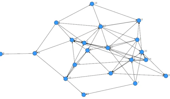
relationships to be portrayed simultaneously at individual and global levels providing rich context for each. Network graphs such as Figure 12.1 (alternatively described as ‘social graphs’ or ‘sociograms’) communicate complicated data powerfully. In this graph, each circle (alternatively described as a ‘node’ or ‘vertex’) represents a social entity, such as an individual staff member in a workplace, a group, an organization, or even a social artefact such as a text.
Each line in the graph (alternatively described as ‘tie’, ‘edge’, or ‘arc’) represents a relationship between two nodes, such as the provision of information. Each node is distinctly identified and is labelled by a number in this case, but names could also be used. The arrows indicate a direction to the relationship; node 7 is providing something (say information) to node 11 but not vice versa. Non-directional relationships can also be plotted, such as where two individuals share an office (formally, ‘arcs’ refer to directional relationships while ‘edges’ refer to non-directional relationships). Finally, the relative importance or value of a node or the strength of a relationship can be represented by differences in the size of the node or width of a line.
One of the powerful communicative features of a network visualization is that it simultaneously presents both specific and general data. Taking node 20, for example, there are specific data about its information flows: 20 receives information from nodes 12, 7, 6, and 14 while it provides information to nodes 8 and 9 and reciprocates with 14. At the same time, the visualization illustrates the flow of information among the workplace as a whole, a lot of information flows being concentrated in the region encompassing nodes 20, 14, and 4; and 15, 2, 12, 17, and 10. Finally, the relative position of node 20 compared to other nodes and the network as a whole is readily apparent. The visualization of the network thus provides a much richer representation of the data than
traditional social science approaches utilizing bivariate or multivariate comparisons.
12.3 WHERE DO THE LINES COME FROM?
Early social network analysis was predominantly undertaken on a small-scale basis via personal interviews. In the example network, a researcher would interview each person in the workplace, asking each in this case, ‘Who in this workplace provides you with information important to complete your work?’ The responses are plotted, with a nomination being represented as a line to the nominator from the person nominated. The complete network of relationships emerges from the triangulation of the responses of all the participants.
Alternative approaches to small-scale data collection include ethnography, where a researcher is located in a social environment and observes and records interactions; and expert panels, where people familiar with an organizational setting are asked to describe interactions they are aware of. For
larger personal networks, structured questionnaires are widely used, increasingly web-based, to reach distant or dispersed participants. Structured questionnaires normally employ a roster of all members of the social environment of interest, prompting each participant to consider their relationship with each of the other members. This helps to overcome recall bias, where respondents typically do not recall their strongest relationships but rather the most salient, those that have had a recent unusual impact on them; without prompting, respondents normally will not cite partners, best friends, or long-standing colleagues (Bernard et al. 1982).
With the rapid growth in the availability of online communication logs, databases, and documentary archives, archival sources and data-mining approaches have become increasingly popular in social network analysis. There is a long tradition of mining official company registers to identify interlocking directors between firms. More recently SNA has been applied to analyse very large data sets of patent registrations to examine collaboration in research and development;
publication citations to study scientific collaboration more generally; hyperlinks between websites to map the World Wide Web and groups within it; and social media interactions such as tweets. Mining of large economic data sets include inter-country and inter-industry trade data to examine core– periphery structures (Smith and White 1992); financial transactions; and news data to study contagion in financial markets (Kyriakopoulos et al. 2009). More traditional archival sources may also provide data for heterodox economic applications; John Padgett has mined parchments to map the social networks underpinning the economy of Renaissance Florence (Padget and Ansell 1993).
Outside very small numbers of nodes, it is difficult to manually and systematically visualize and otherwise analyse social networks, so computer software is employed to analyse network data. For decades, the most widely used SNA software package has been UCINET, originally developed at UC Irvine, Boston College and the University of Greenwich, USA. It maintains its popularity in a similar manner to SPSS in the social sciences more generally; a reasonably accessible user interface, continuous integration of new routines as these are developed in the field, and its ability to readily explore many facets of networks of up to about 5000 nodes.
There are a growing number of alternative packages, generally free and optimized for a specific type of network analysis. For example, Pajek emphasizes its ability to analyse very large
networks (billions of nodes), ORA is designed to analyse multiple networks, Siena is optimized for longitudinal data, NodeXL for social media, Gephi for customized visualizations. Recently there has been a proliferation of SNA programme libraries for program languages, principally for R, but also Python, allowing advanced users to develop highly customized routines for specific analyses (see the SNA library for R and the NetworkX library for Python). All of these packages are readily accessed through a web search.
Whichever software is used for the analysis, there is a common step in preparing the data collected for analysis in such a manner that it can be interpreted as relational data, that is, each data item comprises two nodes and a relationship between them (or not). For all but very large data sets (more than 1 million nodes), this is readily undertaken in a spreadsheet such as Excel. Table 12.1 presents the initial rows of the spreadsheet contacting the data used to generate the network graph in Figure 12.1. This is known as an ‘edgelist’ as it comprises a list of the edges (lines) between nodes in the network. Each row represents an edge between the two nodes listed in columns A and B. More precisely, these are arcs from the node in column A to the node in column B.
<INSERT TABLE 12.1 ABOUT HERE>
This particular way of collecting and recording network data is very simple, versatile, and eases error-checking. In particular, there is normally no need to record the absence of ties, such as between nodes 16 and 10; the nodes listed in the spreadsheet are those with ties, those not listed do not have ties. By default, such a tie is assumed by UCINET to have a value of 1; this value could be recorded in column C and pairs of nodes could be added with a value of 0 representing no tie, but as explained, there is no need to be so pedantic. However, column C can be used to hold information about the strength of the relationship; this might record the number of times information was transferred between nodes in a week, for example, or the value of transactions between two firms. That value can then be used as the basis for the width of the edges in the visualization.
With the data in this format in Excel, it is easy to order them in various ways and use spreadsheet functions to clean the relational data and associated information. For example, Excel’s
pivot table tool can be used to extract a list of each unique node, stored in a second worksheet
alongside various characteristics or attributes of the nodes. Table 12.2 illustrates a node attributes list. The first column lists the node label from the edgelist and the subsequent columns contain
information on three attributes of the node; there can be any number of columns. Thus row 3 concerns the attributes of node 5; it is not female (0), has a salary of 25500 and is in department 1. The values of attributes in this example are all numeric, normally a requirement of SNA software. Note the contrast with the format of the edgelist in Table 12.1: an edgelist holds data about the relationships between pairs of nodes; a node attribute list holds data about the characteristics of each node.
<INSERT TABLE 12.2 ABOUT HERE>
Most SNA software has easy methods for importing data in the formats above, sometimes involving a conversion program. Once imported into SNA software, the network can be quickly visualized and various metrics of the network calculated.
12.4 DATA CONSIDERATIONS
Collecting relational data raises a range of data considerations outside those normally faced by
traditional social science. First, the consistency of the relationship is critical in SNA. Second, there are some particular ethical considerations involved in the collection of data for SNA. Finally, there are a series of important considerations, differing from standard social science approaches, in terms of the boundaries of the sample, the method of collecting the sample, and the response rate.
To analyse a network, the relational data must be consistent: that is, the relationship being measured between nodes 1 and 2 must be the same relationship as the relationship being measured between nodes 2 and 3 and all other nodes in the network. For example, we might ask someone to tell us who they get information from and who they get advice from; while these sound similar it is important not to conflate the two. When information networks and advice networks are mapped separately, they typically have quite different structures; the relationships are related, but distinct
(Cross and Parker 2004). Multiple distinctive relationships are typically analysed by superimposing the visualization of one network on top of another or regressing the variations.
While distinctions between relationships are relatively straightforward to deal with when using archival sources, through the use of explicit and consistent definitions of relevant data, it is more problematic for the design of network questions as respondents may have quite different interpretations of categories being employed. For example, respondents are likely to define ‘friend’ differently; some will define this as very close relationships while others may include passing
acquaintances. Respondents may employ different time periods, for example including a first meeting as important information, while others may focus on information in the last week. Respondents may be reluctant to discuss some relationships; trust is a relationship theorized as important to many economic transactions but in survey situations respondents are often unwilling to reveal who they do or do not trust. Network questionnaires thus need careful design and piloting; questions should be specified within a particular context and time period, for example, ‘How many times in the last week did this person provide you with information important to your work?’ (Laumann et al. 1983).
The sensitivity of network analysis to the specific questions asked in questionnaires highlights another difficulty in data collection: the heightened intrusiveness of the questions. People are not normally asked by social scientists to specify their close personal relationships. Because of this heightened intrusiveness, together with the relative novelty of the techniques, negotiating access to respondents is typically more involved than in traditional social science research. In particular, comprehensive buy-in is needed from the principal decision-makers in organizational settings. There have been numerous cases where data collection has been disrupted by the late intervention by a senior decision-maker who was not sufficiently briefed during the establishment of a project (Cross and Parker 2004).
The heightened intrusiveness also raises a particular range of ethical challenges, as Borgatti and Molina (2003) discuss. Firstly, unlike in most social science research, in SNA it is not possible to offer respondents anonymity because specific personal relationships are the object of study; we are interested in the relationship between ‘Tom’ and ‘Joan’, rather than the relationship between any X and Y. Secondly, respondents may cite relationships with third parties who may not wish to
participate in the study. While respondents are reporting their own perception, they are also reporting shared information: the fact that a relationship exists. Thirdly, it is difficult to offer confidentiality as participants may deduce the identity of individuals from a network position, even when presented in a sociogram with anonymous identifiers. Lastly, obtaining informed consent is difficult because the techniques are new and participants are unlikely to fully anticipate the implications of the information they provide, as compared to a standard questionnaire. These ethical considerations extend to archival sources as well as survey data. When people make use of a social media site or submit forms to a registry they are unlikely to understand that their location in the communication network can be identified and highlighted.
Accordingly SNA researchers need to consider particular methods of protecting the subjects of research from harm, most likely reputational. Some means of mitigating the concerns about social network data are to provide participants with more information than would normally be provided about the techniques before data is collected; pre-collection workshops or extended briefings are effective. This allows participants to judge what sort of information they want to provide and decide how to respond to questions; it allows third parties a greater chance to remove themselves from the study if they wish. Lastly, sociograms should be used judiciously; if the network has very prominent nodes, the data might best be presented differently, such as by numerical tables.
A further important data consideration is the specification of the network boundary. In one sense, everything in society is connected, but for social analysis we need to isolate parts of society for meaningful examination. But where does the network of interest end? Geographic or organizational boundaries may overlook important relationships; for example, customers external to the firm often influence what happens within a firm; transactions among firms in one country may be influenced by their dealings with government agencies and banks in other countries. Cut-off points are often arbitrary; many early studies of interlocking directors examined only the largest 100 or 200 listed firms but these networks look quite different when 500 or 1000 firms or when non-listed companies are included. Using participants’ own definitions of boundaries, such as nominating their most important customers, is vulnerable to the subjectivity problems discussed earlier. The answer to the
boundary definition problem is in the underpinning research design; the boundary needs to have theoretical significance (Laumann et al. 1983).
The sampling strategy also affects the outcome of the analysis; typically positional, reputational, or event approaches are used. Firstly, a positional strategy selects all participants occupying a defined position in a research setting, such as the chief executive officers (CEOs) of the 100 largest firms or all small businesses in Bristol. The limitation of this approach is the boundary definition problem discussed above. Secondly, a reputational strategy selects participants based on an expert panel – knowledgeable informants – who nominate the key people in the research setting. Alternatively, the sample could be selected by snowballing from an initial contact or recommendation, asking these to nominate others for inclusion, who then nominate others. The limitation of the
reputational approach is that it tends to overstate connectedness; respondents are likely to nominate the people they know the best. Thirdly, an event strategy selects respondents who participate in important events. This overcomes the limitations of the other two approaches, but issues remain with selecting the correct event and handling otherwise important participants who may have missed the event for particular reasons (Laumann et al. 1983).
Whichever sampling strategy is adopted, SNA needs high response rates. Unlike statistical social science approaches, completeness of data is important; SNA does not generally use
representative samples because the distributions of ties in networks vary greatly.1 Missing data and false positives can have a large impact on the network structure if this concerns highly connected nodes. Figure 12.1 would look a lot different if node 12 was missing. Archival data, in particular, normally need a great deal of cleaning and checking to make sure that nodes are identified correctly and consistently. When identifying directors who serve on multiple company boards, for example, the challenge is to ensure that ‘J. Smith’ listed on one board is the same person as the ‘J. Smith’ listed on another, and to determine whether this is the same person as ‘J.S. Smith’ or ‘John Smith’ on another; birthdates can help but are not fool proof. Where these are incorrectly identified as the same, a false positive, that part of the network will be erroneously dense; if incorrectly identified as different, a false negative, there will be erroneous gaps in the network. While an entire field of prosopography has
developed around these questions (Stone 1971), the key task is to use clearly documented protocols to ensure identification methods are consistent and rigorous.
Survey data for SNA, where non-response is more likely, typically requires much higher response rates than statistically based social science approaches, but, given this, is reasonably robust to missing data where reciprocation is not required: that is, a tie is assumed if node 1 nominates node 2 even without a response from node 2. Here a 60–70 per cent response rate has been found to provide robust results with < 0.1 error, generally underestimating the number of connections and clusters and overestimating the number of steps between each pair of nodes (Kossinets 2006). For SNA metrics more dependent on the network structure such as closeness and betweenness (discussed below), even 80 per cent response rates would produce error rates of 0.15 and 0.25 respectively (Costenbader and Valente 2003). However, low response rates are not associated with great errors in the ranking of nodes within these metrics; that is, it is possible to robustly identify the nodes within the highest 10 per cent of scores on a wide range of network metrics, even with response rates of 60–70 per cent (Borgatti et al. 2006).
12.5 CENTRALITY
Once an edgelist has been imported into SNA software, the network can be quickly visualized, a wide range of network metrics automatically calculated, and analysis commenced. One of the most intuitive steps in this analysis is to consider which nodes have important positions in the network. Looking at Figure 12.1 there are a number of nodes that appear prominently in the visualization, seeming to be more central to the network than others: nodes 13, 2, 12, 17 and perhaps 15 and 4. However, we can go beyond this intuitive, visual impression and analyse this in a more rigorous, mathematical manner.
First, we can count the number of ties each node has, a metric known as degree centrality, on the basis that the node with the most ties (degree count) to other nodes is likely to be more at the centre of what is going on in that network. Node 12 has the most, with nine ties, followed by nodes 13 and 15, with eight ties each. As the ties in this network are directional, representing provision of information, we can distinguish nodes providing information, arrows pointing out or outdegree centrality from those receiving information, arrows pointing in or indegree centrality. Nodes 12 and 6
have the greatest centrality in terms of outdegree, each providing information to six nodes. Node 13 has the greatest indegree, receiving information from six nodes. In an organizational setting, node 13 might be a supervisor or manager receiving reports.
But these simple counts of ties do not seem to explain the apparent centrality of nodes such as 2, 15, 17, and 4, which seem to be in influential positions in the network. These nodes are one step away from those with high degree centrality, they are connected to well-connected positions, in which case they have access to the major information flows in the organization. This position is known as eigenvector centrality, which is degree centrality, weighted by the degree of the nodes connected to; this is a complex calculation best left to the software. In Figure 12.1 the nodes with the greatest in- and outdegree centrality, 12 and 13, also have the greatest eigenvector centrality, but node 15 comes third and nodes 4 and 2 come fourth and fifth. Nodes 12, 13, and 15 also have the greatest ‘closeness centrality’. Closeness is the minimum number of steps to reach all other nodes by the shortest path. There are 31 steps between these nodes and each of the other nodes, another calculation best done by the software.
So far, the nodes and some of the mathematical properties of the nodes in the middle of the network have been considered, but there are some nodes towards the perimeter of the network, not yet considered, that are contributing to its structure. Node 19, for example, seems to have an important intermediary position between the nodes around node 16 and those around node 6; without it there would be a large gap in the network. This node has high betweenness centrality, that is, it is on the shortest path between more pairs of nodes than any other barring nodes 12 and 15. Taking the direction of the ties into account, that is, the flow of information in this case, node 17 has the next-highest betweenness.
Table 12.3 summarizes the metrics for these prominent nodes (demonstrating that it is possible to report network characteristics avoiding the ethical risks associated with the use of sociograms). As these are identifying influential positions within the social network, they can be interpreted as indicators of social capital (Burt 1992; Lin 2001).
12.6 CLOSURE AND BROKERAGE
The contrast between network metrics that emphasize the cohesive centre of the network (degree, eigenvector, and closeness centrality) and those focused on bridging different parts of the network (betweenness centrality) underpin an important distinction in social network analysis: closure and brokerage. Closed, cohesive groups have long been seen to underpin trust and reciprocation that provide foundations for efficient, non-transactional, reinforcing economic activity, such as Italian industrial districts, the gift economy, and micro-finance (Macauley 1963; Uzzi 1996). But highly cohesive groups can become stuck in their ways, slow to react to external change, overdependent on the central nodes of the group, and become inefficient over time. By contrast, ties that bridge one cohesive group with another provide access to different information and practices that can stimulate creativity and change. This is the classic entrepreneurial situation: combining resources in novel combinations. The nodes located between cohesive groups have brokerage power; information or other resources can only be transferred by means of the broker, for which they can draw a rent. Hansen et al. (2001) note how the distinction echoes March’s (1991) contrast between exploration and exploitation: tight reinforcing networks (closure) facilitate economies of scale and exploitation of ideas and resources, while looser more diverse links with other groups (brokerage) facilitate exploration of new ideas.
The distinction between closure and brokerage has some dynamic implications. Relationships within a cohesive group are likely to be strong, reinforcing, and overlapping, while those in a
brokering situation are more weak, transitory, and vulnerable. But what sort of ties are more valuable: strong or weak ties? In his doctoral thesis, Mark Granovetter (1974) explored how people find jobs, finding that this was not normally a rational search of vacancy listings but rather, perhaps not so surprisingly, through personal referrals. But what was more surprising was that these referrals were not from close ties, such as friends or family. People found jobs through referrals from weak ties: friends of friends and family associates. Granovetter reasoned that cohesive groups of strong ties are likely to know each other’s information already; the source of novel information is outside the closed
group, provided by the weak ties. He famously summarized this theory as ‘the strength of weak ties’ (Granovetter 1973).
Burt (1992) built on this information theory to argue that it was not the brokerage position per se but the act of creating the link between otherwise disconnected groups that introduced new
resource and informational combinations. Disconnected or less connected groups within a network implied there were ‘structural holes’ that could be potentially bridged. Burt (2004) found that individuals who forged bridging ties were more creative (exposed to novel information and
combinations), paid more, promoted more quickly, and happier in their work. But at the same time, the act of creating new ties was to close the hole, creating closure, underpinning a fundamental dynamism to networks.
12.7 SUBGROUPS
We have seen that network analysis simultaneously provides information about individual nodes and the network context in which they are located. An intuitive second step after identifying particularly prominent nodes is to identify the ‘core’ of the network, the group of nodes that seem to dominate the network structure and around which the others revolve and the most distant nodes form a periphery. A fruitful approach to this is to identify the nodes belonging to the highest ‘k-core’, a subgroup where all nodes are connected to each other by a degree of k or more (Seidman 1983). In Figure 12.1 all nodes are connected and have a degree of at least 1, all but node 5 are connected and have a degree of at least 2, and so on. Figure 12.2 highlights the highest k-core: k is 4.
<FIGURE 12.2 ABOUT HERE>
Within the core it is possible to distinguish particularly closely connected groups. In Figure 12.1 there appear to be a large number of connections within the group of nodes 15, 2, 13, and 17 and the group of nodes 4, 14, 2, and 20, and together these more connected groups appear to be important to the structure of the network. Much early SNA undertaken by anthropologists and sociologists
analysis’ (see Scott 2013 for an overview). This draws on the notion that the minimal social structure to exhibit network characteristics – that is, beyond the dyadic relationship possible between two individuals – is a triad, relationships among three individuals. Heider (1958) theorized that triadic relationships such as that among nodes 5, 16, and 19 were relatively unstable: because node 16 is providing information to 5 and 19, it is likely that 5 and 19 will find something in common and eventually form a relationship, a process known as triadic closure. Similarly, the relationship among nodes 1, 15, and 16 is unstable as 1 is providing a lot and 16 is providing nothing to the triad. By contrast, the relationship between nodes 12, 1, and 18 would be characterized as highly stable, a strong triad, because the relationship is reinforcing. So this structural analysis allowed predictions about the dynamics of the network, which has been applied to the analysis of business groups (Rowley et al. 2005). SNA software has extensive capacity to analyse all manner of variations of triads or larger substructures. A difficulty in this approach, however, is that it is difficult to isolate particularly important subgroups as they overlap widely with others. The 12, 1, 18 triad overlaps with two other strong triads – 1, 15, 12 and 1, 2, 12 – and several weaker triads. But the software can produce a list of all combinations.
An alternative approach is to use cluster analysis to separate groups of nodes that are most similar from those that are most dissimilar. Because networks are highly interdependent, attempts to apply hierarchical clustering analysis (discussed in Chapter 9 in this Handbook) generally only separate a few peripheral nodes from the bulk of the network. More recent developments have focused on ‘community detection’, employing algorithms that first separate small differences in the core such as between the group 15, 2, 13, 17 and the group 4, 14, 20. Figure 12.3 presents the results of one of these community detection algorithms, Girvan–Newman (Girvan and Newman 2002). This suggests that nodes 5 and 11 are peripheral, that the groups initially identified visually as related are central to somewhat larger groups, and that a third group (17, 10, 19) can be distinguished. Note that nodes 17, and 13, identified visually as close to 15 and 2, are grouped elsewhere by this algorithm.
12.8 NETWORK CHARACTERISTICS
Not only does SNA provide metrics for characterizing the positions of nodes within networks, methods for identifying subgroups, but there are a range of metrics for distinguishing networks from each other, essentially indicators of network cohesion or ‘knittedness’ (Borgatti et al. 2013).
Traditionally, network density has been widely used as an indicator of cohesion, defined as the number of ties divided by the total possible number of ties. But it is difficult to compare densities of greatly different-sized networks; it is possible that all 20 nodes in our example could be connected to each other, but unlikely that this would occur with 100 nodes, so larger networks tend to have lower densities. So more recently, networks have tended to be compared on multiple measures including average degree, the mean degree of all nodes; average path distance, the mean number of steps for each node to connect to each other; degree centralization, the extent to which the network centres on a single node; compactness, the mean reciprocal of the shortest paths between each pair of nodes; connectedness, the proportion of pairs of nodes that can reach each other (where parts of a network are disconnected); reciprocity, the proportion of directional ties between pairs of nodes that are reciprocated, and transitivity, the proportion of nodes in complete triads 1-2-3-1 (also known as the overall clustering coefficient). Table 12.4 reports these metrics for the example network.
<TABLE 12.4 ABOUT HERE>
A supplementary approach to characterizing networks as a whole draws from the subgroup
characteristics discussed above. A ‘triad census’ measures the distribution of different types of triadic relationships in a network, highlighting the preponderance of stronger or weaker substructures. The distribution is based on the assumption that any three nodes can be connected in 16 different ways, ranging from no connection at all to three reciprocated ties (Holland and Leinhardt 1970). Triad censuses are readily calculated by major SNA software packages.
12.9 HYPOTHESIS TESTING
The analytic techniques discussed above are largely descriptive, though many provide data for specialized micro-sociological theorizing, such as the dynamic implications of reciprocity, closure, and brokerage, and various triad configurations. But two questions typically remain outstanding from a descriptive analysis of network structure or network positions: Is the observed network structure or network position atypical? And is this structure or position related to other observations? For
example, interlocking director networks are highly centralized and banks are very central within these; given the number of nodes and the number of interlocks, is this different from similarly sized networks in other fields? And, given that centrality in such a network is likely to provide
informational advantages, is network centrality of these firms related to financial performance? Traditional statistical techniques used in the social sciences (see Chapter 10 in this Handbook) cannot be used to answer such questions because the distributions of network connections are highly variable, highly sensitive to small changes in parameters, and thus unstandardized, to date. So the standard statistical technique of comparing observed data to standardized distributions (normal, Poisson, and so on) cannot be used to identify atypical phenomena. Secondly, standard regression techniques assume independence of variables, whereas network data is inherently interdependent: connections among nodes are likely to be maintained and reinforced over time through network effects such as popularity and reciprocity. Attempts to employ standard statistical techniques to network data are prone to the identification of spurious associations, generally overstating the effects of connectivity (Borgatti et al. 2013; Snijders et al. 2010).
However, a range of permutation-based regression techniques can be employed to address the limitations of standard statistical techniques when dealing with network data, as no assumptions are needed about the distribution of observations. Standard ordinary least squares (OLS) regression techniques provide the coefficients. But instead of comparing observed data to standardized distributions to determine statistical significance, permutation techniques are used to compare observed data to thousands of random permutations of the observed values (typically 10 000).
Statistical significance is attributed to observations that persistently differ from the randomly
generated network data (Borgatti et al. 2002). Quadratic assignment procedure (QAP) regression is a powerful set of these techniques; exponential random graph models (ERGM) and stochastic actor-oriented models (SOAM) are also widely used. In interlocking directorship studies, there have been mixed results from statistical examinations of the relationship between interlocks and the financial performance of firms. Early OLS-based approaches suggested some relationship between director interlocks and firm financial performance in particular circumstances (Richardson 1987; Mizruchi and Stearns 1994; Cronin and Popov 2005). But Robins and Alexander (2004), employing ERGM
techniques, found the structure of director interlock networks not atypical of random networks of similar size. QAP regression techniques, however, have found a variety of firm financial indicators associated with director interlocks, again in particular circumstances (Cronin 2012, 2013).
12.10 CONCLUSION
Social network analysis, then, provides a rich methodological toolkit for the study of social
relationships, relationships that are often at the heart of questions of interest to heterodox economics. It is used to uncover the meso-level social interactions that are normally elided by structural or agency constructs.
SNA visualization techniques have proved useful in conveying complex data highly
effectively, and in facilitating preliminary analysis of specific and general data simultaneously. With the increasing availability of larger data sets of relational data, however, visualization has been increasingly superseded by analysis of the network metrics, with visualization reserved for the examination of particular micro-interactions. This has been reinforced by methodological advances and the computational power increasingly available to researchers.
Data collection for SNA involves a distinct set of considerations from those usually faced in the social sciences. These include relationship consistency, relational questionnaire design, careful negotiation of access, ethical challenges, boundary specification, sampling strategies, and
completeness. Clearly documented protocols for data collection can save a great deal of time and reduce the need for rework.
A range of node-level metrics allow the consideration of individual positions within a network as a whole. These draw principally from micro-sociological theories of social exchange and social capital, but are useful in developing and testing a wide range of propositions about social dynamics, such as the strength of weak ties and the dynamics of brokerage and closure.
Similarly, micro-sociological theory provides the basis for a set of metrics about the presence and significance of subgroups within a network. Not only do triadic and clique-like micro-structures highlight groups of influential nodes, but in constituting the endoskeleton of a network they influence the social dynamics within the network. Larger groupings of related nodes can be identified by a range of community detection algorithms.
At the macro-network level, a further set of metrics consider the characteristics of the network as a whole, essentially its cohesiveness. These provide a basis for comparing different networks or for considering network change over time. A denomination of the endoskeleton of subgroup structures via a triad census provides a further DNA-type comparator.
Finally, emergent statistical techniques are providing a firmer basis for hypothesis testing with network data than earlier attempts to apply standard statistical approaches in violation of their basic assumptions. QAP regression, ERGM and SAOM modelling provide much more rigorous methods for testing associations involving network data, with further methods regularly being deployed.
SNA is still a rapidly evolving field, methodologically and theoretically. It is reminiscent of the early days of astronomy, where relatively crude instruments first revealed a vast set of hitherto unknown phenomena; as the instruments have improved, more and more phenomena have been revealed and the theories of how these have come to be have developed greatly. The universe of social relations awaits deep exploration and with their central focus on social relationships, heterodox economic approaches are bound to contribute much to this.
REFERENCES
Bernard, H.R., P.D. Killworth, and L. Sailer (1982), ‘Informant accuracy in social-network data V. An experimental attempt to predict actual communication from recall data’, Social Science Research, 11 (1), 30–66.
Borgatti, S.P., K.M. Carley, and D. Krackhardt (2006), ‘On the robustness of centrality measures under conditions of imperfect data’, Social Networks, 28 (2), 124–36.
Borgatti, S.P., M.G. Everett, and L.C. Freeman (2002), ‘Ucinet 6 for Windows: software for social network analysis’, Harvard, MA: Analytic Technologies.
Borgatti, S.P., M.G. Everett, and J.C. Johnson (2013), Analysing Social Networks, London: Sage. Borgatti, S.P. and J.L. Molina (2003), ‘Ethical and strategic issues in organizational social network
analysis’, Journal of Applied Behavioral Science, 39 (3), 337–49.
Brass, D.J. (1992), ‘Power in organizations: a social network perspective’, in G. Moore and J.A. Whitt (eds), Research in Politics and Society, Greenwich, CT: JAI Press, pp. 295–323.
Burt, R.S. (1992), Structural Holes: The Social Structure of Competition, Cambridge, MA: Harvard University Press.
Burt, R.S. (2004), ‘Structural holes and good ideas’, American Journal of Sociology, 110 (2), 349–99. Burt, R.S. and D. Ronchi (1990), ‘Contested control in a large manufacturing plant’, in J. Wessie and
H. Flap (eds), Social Networks Through Time, Utrecht: ISOR, pp. 121–57.
Calvó-Armengol, A. and M.O. Jackson (2004), ‘The effects of social networks on employment and inequality’, American Economic Review, 94 (3), 426–54.
Costenbader, E. and T.W. Valente (2003), ‘The stability of centrality measures when networks are sampled’, Social Networks, 25 (4), 283–307.
Cronin, B. (2012), ‘National and transnational structuring of the British corporate elite’, in J.P. Scott and G. Murray (eds), Financial Elites and Transnational Business:Who Rules the World? Cheltenham, UK and Northampton, MA, USA: Edward Elgar, pp. 177–92.
Cronin, B. (2013), ‘The value of corporate political connnections’, paper presented to the
International Network for Social Network Analysis Conference, Hamburg University, 23 May.
Cronin, B. and V. Popov (2005), ‘Director networks and UK corporate performance’, International Journal of Knowledge, Culture and Change Management, 4 (1), 1195–1205.
Cross, R. and A. Parker (2004), The Hidden Power of Social Networks: Understanding How Work Really Gets Done in Organizations, Boston, MA: Harvard Business School Press.
Eccles, R. (1981), ‘The quasifirm in the construction industry’, Journal of Economic Behavior and Organization, 2 (4), 335–57.
Ferlie, E., L. Fitzgerald, M. Wood, and C. Hawkins (2005), ‘The nonspread of innovations: the mediating role of professionals’, Academy of Management Journal, 48 (1), 117–34. Girvan, M. and M.E.J. Newman (2002), ‘Community structure in social and biological networks’,
Proceedings of the National Academy of Sciences of the United States of America, 99 (12), 7821–26.
Granovetter, M. (1973), ‘The strength of weak ties’, American Journal of Sociology, 78 (6), 1360–80. Granovetter, M. (1974), Getting a Job: A Study of Contacts and Careers, Chicago, IL: Chicago
University Press.
Granovetter, M. (1985), ‘Economic action and social structure: the problem of embeddedness’, American Journal of Sociology, 91 (3), 481–510.
Hansen, M.T., J. Podolny, and J. Pfeffer (2001), ‘So many ties, so little time: a task contingency perspective on corporate social capital in organizations’, Social Capital in Organizations, 18, 21–57.
Heider, F. (1958), The Psychology of Interpersonal Relations, New York: John Wiley & Sons. Holland, P.W. and S. Leinhardt (1970), ‘A method for detecting structure in sociometric data’,
American Journal of Sociology, 76 (3), 492–513.
Ibarra, H. (1992), ‘Homophily and differential returns: sex differences in network structure and access in an advertising firm’, Administrative Science Quarterly, 37 (3), 422–47.
Knoke, D. (1990), Political Networks: The Structural Perspective, New York: Cambridge University Press.
Kogut, B. (2000), ‘The network as knowledge; generative rules and the emergence of structure’, Strategic Management Journal, 21 (3), 405–25.
Kondo, D.K. (1990), Crafting Selves: Power, Gender and Discourses of Identity in a Japanese Workplace, Chicago, IL: University of Chicago Press.
Kossinets, G. (2006), ‘Effects of missing data in social networks’, Social Networks, 28 (3), 247–68. Kyriakopoulos, F., S. Thurner, C. Puhr, and S.W. Schmitz (2009), ‘Network and eigenvalue analysis
of financial transaction networks’, European Physical Journal B, 71 (4), 523–31.
Laumann, E.O. and D. Knoke (1987), The Organizational State: Social Choice in the National Policy Domains, Madison, WI: University of Wisconsin Press.
Laumann, E.O., P.V. Marsden, and D. Prensky (1983), ‘The boundary specification problem in network analysis’, in R.S. Burt and M.J. Minor (eds), Applied Network Analysis, Beverly Hills, CA: Sage, pp. 18–34.
Lin, N. (2001), Social Capital: A Theory of Social Structure and Action, Cambridge: Cambridge University Press.
Macaulay, S. (1963), ‘Non-contractural relations in business: a preliminary study’, American Sociological Review, 28 (1), 55–70.
March, J.G. (1991), ‘Exploration and exploitation in organizational learning’, Organization Science, 2 (1), 71–87.
Mizruchi, M.S. and L.B. Stearns (1994), ‘A longitudinal study of borrowing by large American corporations’, Administrative Science Quarterly, 39 (1), 118–40.
Padgett, J.F. and C.K. Ansell (1993), ‘Robust action and the rise of the Medici, 1400–1434’, American Journal of Sociology, 98 (6), 1259–1319.
Penrose, E.T. (1959), The Theory of the Growth of the Firm, Oxford: Oxford University Press.
Polanyi, K. (1944), The Great Transformation: the Political and Economic Origins of Our Time, New York: Farrar & Rinehart.
Richardson, R.J. (1987), ‘Directorship interlocks and corporate profitability’, Administrative Science Quarterly, 32 (3), 367–86.
Robins, G. and M. Alexander (2004). ‘Small worlds among interlocking directors: network structure and distance in bipartite graphs’, Computational and Mathematical Organization Theory, 10 (1), 66–94.
Rowley, T.J., H.R. Greve, H. Rao, J.A.C. Baum, and A. Shipilov (2005), ‘Time to break up: social and instrumental antecedents of firm exits from exchange cliques’, Academy of Management Journal, 48 (3), 499–520.
Sabatier, P.A. (1987), ‘Knowledge, policy-oriented learning, and policy change: an advocacy coalition framework’, Science Communication, 8 (4), 649–92.
Scott, J.P. (2013), Social Network Analysis: A Handbook, 3rd edn, London: Sage.
Scott, J.P. and P.J. Carrington (eds) (2011), The SAGE Handbook of Social Network Analysis, London: Sage.
Seidman, S. (1983), ‘Network structure and minimum degree’, Social Networks, 5 (3), 268–87. Smith, D.A. and D.R. White (1992), ‘Structure and dynamics of the global economy: network
analysis of international trade 1965–1980’, Social Forces, 70 (4), 857–93.
Snijders, T.A.B., G.G. van de Bunt, and C.E.G. Steglich (2010), ‘Introduction to stochastic actor-based models for network dynamics’, Social Networks, 32 (1), 44–60.
Stone, L. (1971), ‘Prosopography’, Daedalus, 100 (1), 46–71.
Useem, M. (1979), ‘The social organization of the American business elite and participation of corporation directors in the governance of American institutions’, American Sociological Review, 44 (4), 553–72.
Uzzi, B. (1996), ‘The sources and consequences of embeddedness for the economic performance of organizations: the network effect’, American Sociological Review, 61 (4), 674–98.
Table 12.1 Edgelist example A B C 1 16 5 2 1 16 3 15 16 4 16 19 5 1 15
Table 12.2 Node attributes example
A B C D
1 Node Female Salary Department
2 1 1 23 000 1
3 5 0 25 500 1
4 15 1 23 500 2
5 16 1 27 000 3
Table 12.3 Centrality metrics, selected nodes
Node Degree OutDegree Indegree Eigenvector Closeness Betweenness
2 6 2 5 0.263 34 23.7 4 7 3 4 0.273 33 17.8 6 6 3 3 0.213 35 15.9 12 9 6 4 0.359 31 108.1 13 8 4 6 0.345 31 29.4 15 8 4 5 0.315 31 58.9 17 6 2 4 0.246 34 36.0 19 6 4 3 0.169 34 52.9
Table 12.4 Network cohesion metrics Metric Value Average degree 2.85 Degree centralization 0.19 Density 0.15 Connectedness 0.81 Average path distance 2.54 Compactness 0.40 Arc reciprocity 0.14 Transitivity 0.20
NOTE
1.There are, however, emerging statistical techniques enabling controlling for missing data. These involve the comparison of observed network data against what would be expected to be found in randomly generated networks of the same size (see Scott and Carrington 2011).