Bayesian Analysis of Multi-Stratum Designs and Probability-based Optimal Designs with Separation.

(1)

Rahman, Mohammad Lutfor

For additional information about this publication click this link. http://qmro.qmul.ac.uk/jspui/handle/123456789/9106

Information about this research object was correct at the time of download; we occasionally make corrections to records, please therefore check the published record when citing. For more information contact [email protected]

(2)

Multi-Stratum Designs and

Probability-based Optimal

Designs with Separation

Mohammad Lutfor Rahman

School of Mathematical Sciences

Queen Mary, University of London

A thesis submitted for the degree of

Doctor of Philosophy

(3)

(4)

“To Allah belongs whatsoever is in the heavens and the

earth. Verily, Allah, He is Al-Ghani (Rich, Free of all wants),

Worthy of all praise. And if all the trees on the earth were pens and the sea (were ink wherewith to write), with seven seas behind it to add to its (supply), yet the (praiseworthy) Words of Allah would not be exhausted. Verily, Allah is All-Mighty, All-Wise.” Surah Luqman, Al-Quran [31:26-27].

My all praise to Allah (SWT) for keeping me well and having the op-portunity of higher education.

I am thankful to my supervisor Prof. Steven G. Gilmour for his contin-uous support and pragmatic and relaxed supervision that has a great similarity with that caring of my parents who never forced me to do any-thing after my schooling year 4. I am grateful to Dr. Lawrence Pettit who agreed to became my first supervisor officially when Prof. Gilmour left for University of Southampton. I am thankful to Dr. Lawrence for reviewing my thesis and taking care of me in absence of Prof. Gilmour. Thanks to my PhD examiners for their recommendations to improve the quality of the thesis after the first submission.

I am grateful to my wife Lisa and lovely daughter Zahra for their long patience and support throughout my studies.

I love Queen Mary including its staff for their continuous cordial sup-port and also for funding me through the DTA scholarship during this study. I am thankful to Dr. Peter Zemroch and Pauline Ziman for ad-vising me during ImpactQM knowledge transfer project at Shell Global Solutions UK. I am grateful to Prof. Peter Goos, University of Antwerp, Belgium, for his collaboration with us and allowing us to use data from

(5)

I would like to acknowledge University of Dhaka for the approval of my study leave for the whole period of PhD research.

I am thankful to my students who became colleagues later particularly Iftakhar and Zakir, friends Shihan and Li to have great gossips along with teas, coffees, biscuits, custard doughnuts and so on within the School of Mathematical Sciences building regularly for the last couple of years. These mind refreshing events would never be forgotten for the rest of my life.

Last but not the least, thanks to my great parents who are endless source of my inspiration for encouraging me to keep going my academic studies up to the PhD level.

(6)

Industrial experimental design is an important area under design of experiments and factorial design hold a firm place in industrial experi-ments. The generalization of factorial designs results in split-plot type designs when complete randomization of runs is not possible. More specifically, hard-to-set factors lead naturally to split-plot type designs and mixed models. Mixed models are used to analyze multi-stratum designs as each stratum may have a random effect on the responses. The study of random effects in mixed models might be difficult using likelihood methods because of small number of groups or whole plots in multi-stratum and split-plot designs. Also, zero estimates of variance components could be due to estimating multiple variance components in a hierarchical model. Therefore, likelihood-based inference is often unreliable with the variance components being particularly difficult to estimate for small samples. A Bayesian method considering some non-informative or weakly non-informative priors for variance components could be a useful tool to solve the problem.

Fuel economy experiments, conducted by Shell Global Solutions UK, fall under small sample trap during variance components estimation. Using SAS procedure MIXED, experimenters estimated the variance components to be zero which were unrealistic. Also, the experimenters were unsure about the parameter estimates obtained by likelihood method from linear mixed models. Therefore, we looked for an alternative to compare and found the Bayesian platform to be appropriate. Bayesian methods assuming some non-informative and weakly informative priors enable us to compare the parameter estimates and the variance com-ponents. Profile likelihood and bootstrap based methods verified that Bayesian point and interval estimates are not absurd. Also, simulation studies have assessed the quality of likelihood and Bayesian estimates in this study.

(7)

to a good adhesion to various coatings. The effects of several ad-ditives were also studied in addition to the plasma treatments. The likelihood-based estimates were not reliable completely due to the ex-istence of moderate number of whole-plots. Also, some of the variance components due to batch were zero for some coatings. Assuming non-informative priors for fixed effects and some weakly non-informative priors for variance components we have obtained more sensible estimates of variance components which were inestimable or poorly estimated by the likelihood-based method using SAS procedure GLIMMIX. In this study, the Bayesian methods appeared to give comparable results with classical methods.

One response variable in the polypropylene experiment was categorical which was converted to binary to see the effects of additives on the outcome of interest. Unfortunately for binary responses we failed to obtain estimates of the logistic parameters for some of the coatings as the system did not converge. One of the reasons for this was due to having the separation problem in the data. When one or more explana-tory variables completely separate the responses, the problem is known as separation. This problem causes the non-existence of likelihood es-timates of logistic regression parameters.

We have done some novel methodological works on the separation is-sue to minimize the problem in the light of optimal design techniques. Though the information based D-optimality criterion is widely used in practice, it fails to handle the separation problem appropriately. We have proposed new probability-based optimality criteria to handle the separation problem at the design stage of a study. Our proposed criteria

Ps- and DPs- might be worthwhile to take into account reduction of the

separation problem. However, Ps-criterion alone is not suitable to deal

with separation problem as it produces worse designs in terms of preci-sion of the parameter estimates, i.e. with respect to D-optimality. On

(8)

sensitive to parameter misspecification, pseudo-Bayesian design

crite-rion DPSB- has been proposed. Simulation studies have verified that

Bayesian designs perform better than non-Bayesian designs by provid-ing less bias, less median squared errors and above all less probability of separation. Thus, newly devised Bayesian and non-Bayesian design criteria could be useful in practice to control separation problem at the design stage of a study.

(9)

Contents vii

List of Tables xi

List of Figures xv

1 Introduction 1

1.1 Preface . . . 1

1.2 Problems Addressed in the Thesis . . . 4

1.3 Literature Review . . . 7

1.3.1 Bayesian Analysis of Data from Multi-Stratum and Split-plot Designs . . . 7

1.3.2 Non-existence of Maximum Likelihood Estimates and Sepa-ration Problem in Logistic Regression . . . 9

1.4 Structure of Thesis . . . 14

2 Analysis of Fuel Economy Experiments Using Bayesian Methods 15 2.1 Introduction . . . 15

2.2 Bayesian Models . . . 16

2.3 Bayesian Inference . . . 17

2.4 Markov Chain Monte Carlo (MCMC) . . . 18

2.4.1 Why MCMC in Bayesian Methods? . . . 18

2.4.2 Three Related Terms . . . 18

2.4.3 Gibbs Sampling . . . 19

2.4.4 Software to Implement MCMC . . . 20

2.5 Case Studies . . . 21

2.5.1 Fuel Economy Experiments . . . 21

(10)

2.5.1.2 Contrast: T-B . . . 23

2.5.1.3 Contrast: B2-B1 . . . 27

2.5.1.4 Contrast: (T-B)-(B2-B1) . . . 28

2.5.1.5 Nested Models . . . 30

2.5.2 Round Robin Experiments . . . 31

2.5.2.1 Round Robin Analysis for Fuel A . . . 33

2.5.2.2 Round Robin Analysis for Fuel B . . . 34

2.6 Convergence and MCMC . . . 34

2.6.1 Convergence Diagnostics for Fuel Economy Experiments . . 35

2.6.2 Convergence Diagnostics for Round Robin Experiments . . . 39

2.7 Robustness of Posterior Distributions in Round Robin Experiments 42 2.8 Likelihood Methods in Fuel Economy Experiments . . . 43

2.8.1 Contrast: T-B . . . 43

2.8.2 Contrast: (T-B)-(B2-B1) . . . 44

2.9 Profile Likelihood and Confidence Intervals . . . 45

2.10 Simulation Studies . . . 48

2.10.1 Performance Measures in Simulation Studies . . . 48

2.10.2 Determination of Simulation Size . . . 52

2.10.3 Simulation Studies on Fuel Economy Experiments . . . 52

2.10.4 Robustness of Likelihood and Bayesian Estimators . . . 61

2.10.5 Simulation Studies on Round Robin Experiments . . . 61

2.10.6 Kernel Density of Simulated Estimates . . . 65

2.11 Conclusion . . . 69

3 Bayesian Analysis of Categorical Data from Multi-Stratum Ex-periments 74 3.1 Introduction . . . 74

3.2 Models to be Used in the Analysis . . . 75

3.3 Model Selection . . . 76

3.4 The Polypropylene Industrial Experiment . . . 77

3.4.1 What is Polypropylene? . . . 77

3.4.2 Underlying Design . . . 77

3.5 Binary Response Data Analysis . . . 80

3.5.1 Binary Response Analysis of Coating 1 . . . 82

(11)

3.5.6 Remarks on Mixed Binary Logit Analysis of Coatings . . . . 87

3.6 Ordinal Response Data Analysis . . . 88

3.6.1 Ordinal Response Analysis of Coating 1 . . . 89

3.6.2 Ordinal Response Analysis for Coating 2 . . . 91

3.6.6 Remarks on Mixed Cumulative Logit Analysis of Coatings . 94 3.7 Combined Analysis of Coatings . . . 96

3.8 Investigation of Variance Components with Different Priors . . . 103

3.9 Convergence Diagnostics . . . 104

3.10 Profile Likelihood, Confidence Intervals and Simulation Studies . . . 108

3.11 Conclusion . . . 111

4 Optimal Design for Categorical Data Minimizing the Probability of Separation 114 4.1 Optimal Design in Statistics . . . 114

4.2 Separation Problem in Categorical Data Analysis and Non-existence of Maximum Likelihood Estimates . . . 115

4.2.1 Types of Separation . . . 116

4.2.2 Hypothetical Example of Separation . . . 117

4.2.3 Separation Problem in the Current Study . . . 117

4.2.4 Non-existence of Maximum Likelihood Estimates . . . 118

4.3 Existing Ways of Dealing with the Separation Problem . . . 121

4.3.1 Solutions for Quasi-complete Separation . . . 122

4.3.2 Solutions for Complete Separation . . . 122

4.4 Probability of Separation . . . 123

4.4.1 Probability of Complete Separation . . . 125

4.4.2 Probability of Quasi-complete Separation . . . 125

4.4.3 Theorem . . . 126

4.4.4 Numerical Example: Reduction of Probability of Separation with the Minor Changes in Design Points . . . 129

4.5 Probability of Quasi-complete Separation with Two or Three Equal Design Points Successively . . . 130

4.6 Sequential Method to Compute Probability of Separation . . . 132

(12)

4.7.1 Ps-optimality Criterion . . . 133

4.7.2 Compound Criteria and DPs-optimality . . . 134

4.8 Local Optimization of DPs-optimality Criterion . . . 136

4.9 DPs-optimal Designs for Models with More Than One Factor . . . 137

4.10 Comparing Results from Various Designs . . . 138

4.10.1 Comparing D- and Ps-optimality from D-, Ps, DPs-optimal designs . . . 138

4.10.2 Size of D-, Ps-, and DPs-optimal designs . . . 143

4.10.3 D-and P-efficiencies of D-, Ps, and DPs-optimal designs . . . 145

4.10.4 DPs-optimal designs with different choice of mixing constantα147 4.10.5 DPs-optimal designs with different sizes . . . 151

4.11 Sensitivity Analysis . . . 153

4.12 Simulation Studies on DPs-optimal Designs . . . 157

4.13 Pseudo Bayesian Designs . . . 165

4.14 Conclusions . . . 169

5 Discussion and Conclusion 173 5.1 Introduction . . . 173

5.2 Fuel Economy Experiment . . . 174

5.3 Polypropylene Experiment . . . 175

5.4 Optimal Design with Separation . . . 177

5.5 Conclusions and Future Research . . . 179

Appendix 181

(13)

2.1 Underlying design in the fuel economy experiment . . . 22

2.2 Data before averaging over back-to-back tests . . . 24

2.3 Data averaged over back-to-back repeats . . . 25

2.4 Data to test contrast T-B . . . 25

2.5 Results for contrast T-B . . . 27

2.6 Results for contrast B2-B1 . . . 28

2.7 Data for contrast(T-B)-(B2-B1) . . . 29

2.8 Results from contrast (T-B)-(B2-B1) . . . 30

2.9 Results from the nested model . . . 31

2.10 Round Robin data . . . 33

2.11 Round Robin results of fuel A . . . 34

2.12 Round Robin results of fuel B . . . 34

2.13 Robustness of estimates with different priors . . . 42

2.14 Linear Mixed-effects model fit for (T-B) by REML method . . . 43

2.15 Linear Mixed-effects model fit for (T-B) by ML method . . . 44

2.16 Linear Mixed-effects model fit for (T-B)-(B2-B1) by REML method 44 2.17 Linear Mixed-effects model fit for (T-B)-(B2-B1) by ML method . . 45

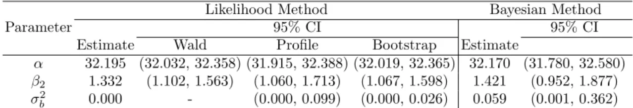
2.18 Likelihood and Bayesian estimates with 95% confidence/credible in-tervals under different methods in fuel economy experiment . . . . 47

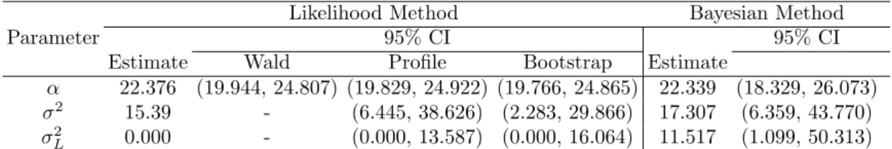
2.19 Likelihood and Bayesian estimates with 95% confidence/credible in-tervals under different methods in round robin experiment for fuel A . . . 48

2.20 Simulated performance of maximum likelihood and Bayesian esti-mates in fuel economy experiments assuming true parameter val-ues as α = 32, β2 = 1.4, σ2b = 0.05; priors as α ∼ N(0,0.001), β2 ∼N(0,0.001); and sample size n=6 . . . 53

(14)

2.21 Simulated performance of likelihood and Bayesian estimates in fuel

economy experiments. True parameter values: α = 32, β2 = 1.4,

σ_b2 = 0.05; Priors: α ∼ N(0,0.001), β2 ∼ N(0,0.001); simulation

size=2000, n=40 . . . 57

2.22 Performance of likelihood and Bayesian estimates in fuel economy experiments considering different size of simulations. True

param-eter values: α = 32, β2 = 1.4, σ2b = 0.05; Priors: α ∼ N(0,0.001),

β2 ∼N(0,0.001); n=40 . . . 59

2.23 Robustness of likelihood and Bayesian estimates in fuel economy

experiments with different values of σ2 and σ2_b where true parameter

values are α = 32 and β2 = 1.4, and priors given α ∼ N(0,0.001)

and β2 ∼N(0,0.001); simulation size=2000, n=40 . . . 60

2.24 Simulated performance of likelihood and Bayesian estimates in round

robin experiments. True parameter values: α=22, σ2₌₁₆ _σ2

L=5,

r=11.2, R=12.831 ; simulation size=2000, n=20 . . . 62

2.25 Simulated performance of likelihood and Bayesian estimates in round

robin experiments. True parameter values: α=22, σ2₌₁₆ _σ2

L=5,

r=11.2, R=12.831 ; simulation size=2000, n=40 . . . 63

3.1 Levels of factors studied in the polypropylene experiment . . . 78

3.2 Frequency distribution of ASTM scores in the polypropylene

exper-iment . . . 80

3.3 Classical and Bayesian estimates obtained from mixed binary logit

model for coating 1 . . . 83

3.8 Classical and Bayesian estimates obtained from mixed cumulative

logit model for coating 1 . . . 90

(15)

logit model for coating 3 . . . 93

3.11 Classical and Bayesian estimates obtained from mixed cumulative logit model for coating 4 . . . 94

3.12 Classical and Bayesian estimates obtained from mixed cumulative logit model for coating 5 . . . 95

3.13 Likelihood-based and Bayesian estimates... all coatings . . . 100

3.14 Investigation of variance components with different priors . . . 104

3.15 Standard deviation and Monte Carlo error (MC Error) in Bayesian analysis of coating 2 . . . 105

3.16 Likelihood and Bayesian estimates with 95% intervals under different methods . . . 109

3.17 Simulated performance of maximum likelihood and Bayesian esti-mates under binary logit model in polypropylene experiments as-suming true parameter values as β0 = 3.6, β1 = 1, β2 = 1.7,β3 = 1.5,β4 = 2.3,β5 = 3.2, σ2δ = 3, σ2 = 4.2; and sample size n=300 . . . 110

4.1 Hypothetical examples of separation problem . . . 117

4.2 Existence of separation problem in the current study . . . 118

4.3 Hypothetical examples of overlapped and separated data . . . 119

4.4 Data and design matrix . . . 124

4.5 Probability of complete separation at X3 =X∗ . . . 130

4.6 Probability complete and quasi-complete separations at X3 =X∗ . 130 4.7 Separation with two equal successive design points . . . 131

4.8 Compound method to compute separation probability . . . 132

4.9 Comparing D- and Ps-optimality from D-optimal designs . . . 139

4.10 Comparing D- andPs-optimality from Ps-optimal designs . . . 140

4.11 Comparing D- and Ps-optimality from DPs-optimal designs with α = 0.5 . . . 141

4.12 Comparing D- and Ps-optimality from DPs-optimal designs with different α . . . 148

4.13 Sensitivity index of DPs-optimal designs with design size 16 . . . . 156

4.14 Sensitivity index of DPs-optimal designs with design size 20 . . . . 156

4.15 Simulated performance of mean estimates from DPs designs with 10,000 simulations . . . 158

4.16 Simulated performance of estimates from DPs designs with 10,000 simulations, n=8 . . . 160

(16)

4.17 Simulated performance of estimates from DPs-designs with 10,000

simulations, n=16 . . . 161

4.18 Simulated performance of estimates from DPs designs with 10,000

simulations, n=8 . . . 162

4.19 Simulated performance of estimates DPs-designs with 10,000

simu-lations, n=16 . . . 163

4.20 Bayesian designs . . . 164

4.21 Simulated performance of estimates in Bayesian designs with 10,000

simulations, True parameters: β0 = 0, β1 = 1 . . . 167

4.22 Simulated performance of estimates in Bayesian designs with 20,000

(17)

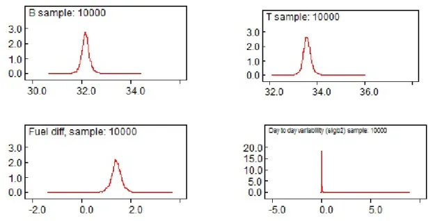
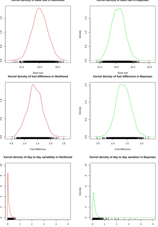
2.1 Kernel densities of parameters in fuel economy experiment; Base fuel

(B) (top left), Test fuel (T) (top right), Fuel Difference β2 (bottom

left), Day to day variability (σ2

b) (bottom right). . . 35

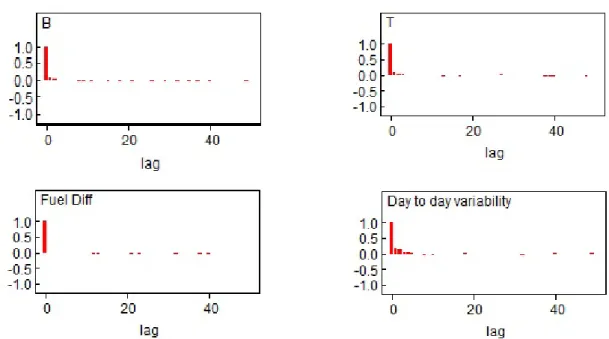
2.2 Autocorrelation of parameters in fuel economy experiment; Base fuel

left), Day to day variability (σ2

2.3 History plot of parameters in fuel economy experiment; Base fuel

left), Day to day variability (σ2_b) (bottom right). . . 37

2.4 Gelman Rubin statistics of parameters in fuel economy experiment;

Base fuel (B) (top left), Test fuel (T) (top right), Fuel Difference β2

(bottom left), Day to day variability (σ2

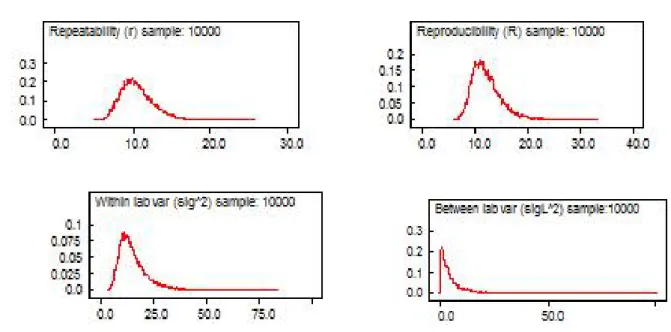
2.5 Kernel densities of parameters in round robin experiments;

Repeata-bility (r) (top left), ReproduciRepeata-bility (R) (top right), Within lab

vari-ability (σ2_{) (bottom left), Between lab variability (}_σ2

L) (bottom right). 39

2.6 Autocorrelation of parameters (before thinning) in round robin

ex-periments; Repeatability (r) (top left), Reproducibility (R) (top

right), Within lab variability (σ2) (bottom left), Between lab

vari-ability (σ_L2) (bottom right). . . 40

2.7 Autocorrelation of parameters (after thinning) in round robin

exper-iments; Repeatability (r) (top left), Reproducibility (R) (top right),

Within lab variability (σ2_{) (bottom left), Between lab variability}

(σ2

L) (bottom right). . . 40

2.8 History plot of parameters in round robin experiments; Repeatability

(r) (top left), Reproducibility (R) (top right), Within lab variability

(σ2_{) (bottom left), Between lab variability (}_σ2

(18)

2.9 Gelman Rubin (GR) statistics of parameters in round robin experi-ments; Repeatability (r) (top left), Reproducibility (R) (top right),

Within lab variability (σ2) (bottom left), Between lab variability

(σ2

L) (bottom right). . . 41

2.10 Kernel density of simulated parameter estimates in fuel economy

experiments; base fuel (α)(top), fuel difference (β2) (middle), day to

day variability (σ2

b) (bottom) . . . 66

2.11 Kernel density of simulated parameter estimates in fuel economy

experiments; Base fuel (α)(top), Fuel difference (β2) (middle), Day

to day variability (σ_b2) (bottom) . . . 67

2.12 Kernel density of simulated parameter estimates in round robin ex-periments; within lab variability (top left), between lab variability

(top right), repeatability (bottom left), reproducibility (bottom right) 68

2.13 Kernel density of simulated parameter estimates in round robin ex-periments; within lab variability (top), between lab variability

(sec-ond from top), repeatability (third from top), reproducibility (bottom) 70

3.1 Factors and stages in the polypropylene experiment . . . 79

3.2 Hasse diagram for combined analysis . . . 97

3.3 Kernel density of few a parameters of the best model for coating 2;

EPDM (top left), Ethylene (top right), Batch (bottom left), Run

(bottom right). . . 106

3.4 Trace plots of a few parameters of the best model for coating 2;

EPDM (top left), Ethylene (top right), Batch (bottom left), Run

(bottom right). . . 106

3.5 Autocorrelation status of few parameters after thinned as 20th for

coating 2; EPDM (top left), Ethylene (top right), Batch (bottom

left), Run (bottom right). . . 107

3.6 History plot of few parameters of the best model corresponding to

coating 2; EPDM (top left), Ethylene (top right), Batch (bottom

left), Run (bottom right). . . 107

3.7 Gelman-Rubin statistic of few parameters of the best model

corre-sponding to coating 2; EPDM (top left), Ethylene (top right), Batch

(bottom left), Run (bottom right). . . 108

4.1 Log-likelihood as a function of the slope under separation . . . 120

(19)

4.3 D-criterion in D-, Ps, and DPs-optimal designs . . . 144

4.4 D-and P-efficiencies in D-optimal designs with various sizes . . . 145

4.5 D-and P-efficiencies in Ps-optimal designs with various sizes . . . . 146

4.6 D-and P-efficiencies in DPs-optimal designs with various sizes given

that α= 0.5 . . . 146

4.7 D-efficiencies in D-,Ps, and DPs-optimal designs . . . 147

4.8 P-efficiencies in D-,Ps, and DPs-optimal designs . . . 149

4.9 Probability of separation Vs size of DPs-optimal designs with variousα150

4.10 P-efficiencies Vs size of DPs-optimal designs with various α . . . 150

4.11 D-criterion Vs size of DPs-optimal designs with various α . . . 151

4.12 D-efficiencies Vs size of DPs-optimal designs with various α. . . 152

4.13 Probability of separation Vs mixing constant (α) from DPs-optimal

designs with different sizes . . . 152

4.14 D-criterion Vs mixing constant (α) from DPs-optimal designs with

different sizes . . . 153

4.15 P-efficiency Vs mixing constant (α) from DPs-optimal designs with

different sizes . . . 154

4.16 D-efficiency Vs mixing constant (α) from DPs-optimal designs with

(20)

Introduction

1.1

Preface

Undertaking experiments is a natural way to realize the best way to do things. It is a common phenomenon to do experiments in any scientific discipline for striving towards perfection. Statistical experimental designs attempt to answer how, with a minimum of effort, one can discover which factors do what to which responses. In other words, experimental design or design of experiments is a structured and organized way to conduct and analyze controlled tests for evaluating the factors that affect response variables.

Design of experiments was pioneered by Ronald A. Fisher in the 1920s and early 1930s at Rothamsted Experimental Station, an agricultural research station 25 miles north of London. Fisher recognized that flaws in the way in which the exper-iment that generated the data had been performed often hampered the analysis of data from agricultural systems. With the interactions of scientists and researchers in various fields, he developed the insights that led to the three basic principles of experimental design: randomization, replication, and blocking. Randomization means random assignment of experimental units to the levels of a treatment. It helps distributing the unusual characteristics of experimental units over the treat-ment levels so that they do not selectively bias the outcome of the experitreat-ment. Random assignment also allows the computation of an unbiased estimate of error effects which are not attributable to the manipulation of the independent variable and it makes sure that the errors are statistically independent. Replication is the

(21)

of treatment effects. Blocking is an experimental procedure for isolating variation attributable to an extraneous factor. Blocking helps to remove the influence of extraneous factors as extraneous factors are undesired sources of variation that can

affect the response variable [Montgomery, 2008].

Although the experimental design technique was first used in an agricultural con-text, the technique has been extended successfully in industry since the 1940s. The industrial experimental era was catalyzed by the introduction of response surface methodology (RSM) by Box and Wilson in 1951. They identified the fundamental differences between agricultural and industrial experiments. In industrial exper-iments, the response variable can be observed shortly after the experiment and experimenter can learn quickly important information from a small group of runs that might be utilized to plan the next experiment. The RSM technique was widely used in the chemical and process industries, particularly in research and

develop-ment works. Taguchi et al. [1987] advocated for robust parameter designs

specif-ically in making processes insensitive to environmental or other factors, obtaining products insensitive to variation transmitted by factors, and finding levels of the process variables that force the mean to a desired value while simultaneously

reduc-ing variability around this value [Montgomery,1999]. However, Taguchi’s methods

were criticized widely as his methods were advocated primarily by entrepreneurs in the West and as the underlying statistical science had not been adequately peer

reviewed [Montgomery, 2008]. Though Taguchi’s methods were criticized, his

ef-forts appeared to have positive impacts by instigating designed experiments in the discrete part industries including automotive and aerospace manufacturing, electronics and semiconductors, and many other industries that had little use of experimental design techniques.

Applications of designed experiments have grown substantially in industries. More or less industrial experimental design techniques have some common approaches to follow. The following steps are useful while one may be performing an industrial experiment.

1. Identification and statement of the problem. 2. Selection of the response variable.

(22)

4. Determination of factor levels and range of factor settings. 5. Choice of appropriate experimental design.

6. Experimental planning and performing the experiment.

7. Statistical data analysis, interpretation and recommendations.

The above points are self explanatory and yet further details on these are also

available inAntony and Capon [1998] and Montgomery [2008].

Though experimental design techniques are very powerful but there are some prob-lems associated to implementation of the techniques to industries. In many situ-ations, there is lack of communication between the industrial and the academic worlds, therefore it limits the use of experimental design in many manufacturing industries. There is also lack of adequate skills and expertise required by engineers in manufacturing to define and formulate problems. Thus many engineers face dif-ficulties in analysing a particular process quality problem and then converting the engineering problem into statistical terms from which appropriate solutions can be chosen. Further, even after accomplishing experiments, problems may arise from a statistical point of view, e.g. parameter estimates may not exist due to censoring in

lifetesting experiments particularly connected to small experiments [Hamada and

Tse, 1992]. Due to small number of units often estimates of some parameters, e.g.

variance components in mixed models, might not be estimable reliably. Further, due to the nature of the data, computational obstacles may arise, for instance, maximum likelihood estimates (MLEs) may not exist for particular types of mod-els under designed experiments. However, despite these deficiencies, experimental designs are increasingly advancing in industrial experiments as they catalyze sci-entific methods and greatly increase efficiency in industrial production in terms of less cost, less time and better quality.

In the field of industrial experimental designs factorial designs hold a firm place. A researcher selects a fixed number of levels of each of the factors in a factorial design and then runs the experiment with all possible combinations. If the researcher is unable to randomize completely the order of runs that results in generalizations

(23)

not possible often in industrial experiments because some factors may have levels that are difficult to set. If hard-to-set factors are considered at the design stage, they lead naturally to multi-stratum structures, with different factors applied in

different strata through restricted randomization, as in split-plot designs [Goos and

Gilmour, 2012]. Further, many split-plot designs yield categorical response data. The combination of categorical data and restricted randomization necessitates the use of generalized linear mixed models as each stratum under multi-stratum de-signs may have random effects on the responses.

The study of random effects in mixed models is often difficult because of small number of groups (number of strata or whole plots in multi-stratum and split-plot designs), particularly difficulties with the estimation of variance components and consequently with the statistical inference. To avoid these difficulties of estimation, Bayesian analysis is suggested by earlier researchers for normal responses assum-ing some non-informative or weakly informative priors for the relevant parameters. This is extended to discrete responses in this Thesis.

During logistic regression analysis of binary or categorical response data in exper-iments, researchers often face convergence difficulties due to a problem known as ‘separation’. It is an undesirable problem in models for dichotomous dependent variables. It occurs when one or more model covariates perfectly predicts some binary outcome. Current literature suggests that researchers need to compromise

with separation either by undertaking post hoc data adjustment or by estimation

corrections. However, apart from these solutions, the separation issue could be handled by using newly developed optimality criteria at the design stage of an experiment.

1.2

Problems Addressed in the Thesis

There are two main issues in this Thesis. Firstly, estimation of variance compo-nents that were poorly estimated or estimated as zero in multi-stratum industrial experiments. Secondly, handling separation problem that causes infinite estimates

(24)

Bayesian techniques as an alternative to likelihood based methods and for separa-tion problem we have used an optimal design technique to avoid separasepara-tion at the design stage of a study. However, the two things - non-existence of MLE (or infinite estimates) of parameters and zero estimates of variance components should not be confused and should be treated as two separate issues- former is about random effects and latter is about fixed effects. Bayesian methods implemented here are not to show outright domination over frequentist methods, rather we consider as complementary to each other and where frequentist (likelihood) methods fail then Bayesian methods appeared to assist or vice versa.

Increasingly analysis becomes cumbersome for complex models. Often researchers want to compare results by applying several methods. The likelihood estimates of variance components were zero in fuel economy and polypropylene industrial exper-iments. The main reason of having zero estimates is small to moderate number of

experimental units. Also Bayarri and Berger [2004] have clarified that maximum

likelihood estimates of variance components in hierarchical models (or variance components models) can easily be zero, especially when there are several variance components in the model that are being estimated. It is also quite common in problems with numerous variance components to have at least one MLE variance estimate equal to zero. Therefore, as the likelihood (frequentist) method fails we consider Bayesian method as an alternative to obtain realistic estimates of vari-ance components. But appropriate choice of priors is crucial in Bayesian analysis.

Bayarri and Berger [2004] noted that frequentists are usually not interested in subjective, informative priors, and on the other hand Bayesians are less likely to be interested in frequentist evaluations when using subjective, highly informative priors. Again the most common scenarios of useful connections between frequen-tists and Bayesians are when no external information (other than the data and the model itself) are introduced into the analysis - in the Bayesian context, when “objective prior distributions” are used. As we do not have firm basis to consider any informative priors, we have implemented non-informative or weakly informa-tive priors throughout our analysis of fuel economy and polypropylene experiments to keep things close to frequentist ideas. However, performance of the Bayesian and the likelihood based estimates has been assessed through simulation studies.

(25)

adapt the methodology to a new application area. On the basis of this experi-ence from the Bayesian study of polypropylene experiment, we had an opportunity to work for Shell Global Solutions UK, an energy consultant and technology in-novator, through a knowledge transfer project called ‘ImpactQM Shell Transfer Project’ that produces the second chapter in the Thesis. This is a pioneering re-search where we have applied Bayesian methods in the fuel efficiency field, which has also a particular feature of using very small experiments. This method is now recommended in the Shell industrial guidelines. Finally, a statistical computational problem known as ‘separation’ arises during binary response analysis under logis-tic regression that leads us do some novel methodological works on optimal design of experiments considering separation issues. The rest of this section elaborates slightly on the topics that we studied.

In a fuel economy experiment, researchers wanted to analyze data in different ways as they were unsure which methods to adopt in practice. This experiment was run as a multi-stratum design as there were several strata (sessions-morning vs afternoon, days nested under weeks) in the experiment. Initially they applied likelihood-based methods, particularly linear mixed models to model the continu-ous responses. The purpose was to compare performances of car fuels. However, variance components due to random effects were estimated as 0 which was unreal-istic. In their further investigation, they found the Bayesian method as a possible

alternative described inGilmour and Goos [2009] to estimate the variance

compo-nents. Assuming some weakly informative priors on the variance components, the problem can be resolved, thus estimating the parameters and their standard errors more precisely. Simulation studies were accomplished to determine which method likelihood or Bayesian produces better estimates and further which set of priors produces the best estimates. The quality of point estimates was assessed by bias, relative bias, mean and median square errors and quality of interval estimates was measured by the coverage probabilities, average and median widths of the confi-dence/credible intervals.

Generalized linear models (GLMs) are widely used to analyze categorical response data, including in factorial designs. The combination of categorical data and

(26)

re-ponents of a mixed model depends on the number of whole plots in a split-plot design. An inadequate number of whole plots is a hindrance in the proper esti-mation of variance components. In the polypropylene industrial experiment, the number of whole plots (batches) was moderate, therefore, the experimenters could

not estimate a variance component accurately [Goos and Gilmour,2012]. However,

a Bayesian method assuming some weakly informative priors for variance compo-nents was suggested to overcome the hurdle. In this study, we have implemented the Bayesian techniques to estimate the variance components that were inestimable or poorly estimated in likelihood-based methods.

When responses are binary, then often it might be impossible to obtain maximum likelihood estimates (MLEs) of the logistic model parameters due to convergence difficulties. This happens due to a problem known as ‘separation’ that occurs due to the perfect prediction of outcome of interest by one or more covariates. It is a phenomenon associated with models including logistic and probit models for binary or categorical outcomes. We have carried out a study on the separation issue in the context of optimal design theory.

1.3

Literature Review

In this section, some literature have been reviewed that will help understanding the background of this study.

1.3.1

Bayesian Analysis of Data from Multi-Stratum and

Split-plot Designs

In some multi-factor experiments complete randomization is not feasible. This of-ten results in a generalization of the factorial design called the split-plot designs. A split-plot design is a blocked experiment, where blocks themselves serve as experi-mental units for a subset of the factors. The blocks are referred to as whole plots, while the experimental units within blocks are called split plots, split units or

(27)

may have random effects on the responses.

Letsinger et al.[1996] pointed out that the results from data analysis of split-plot response surface designs could be misleading if experimenters ignore the multi-stratum structure. For normal responses, they recommended the use of a linear mixed model with variance component parameters estimated by residual maxi-mum likelihood (REML) and fixed effect parameters by empirical generalized least squares (GLS). This has become the standard way of analysing data from indus-trial multi-stratum experiments and is usually successful if there are ample residual degrees of freedom in each stratum.

A disadvantage of REML-GLS estimation is that it can give highly undesirable and misleading conclusions in non-orthogonal split-plot designs with few main plots.

This proved to be true in a freeze-drying coffee experiment reported by Gilmour

et al. [2000] where the main plot variance component was estimated to be 0 using REML-GLS methods. Experience suggested that this was implausible, but

infer-ences and estimated standard errors for fixed effects use this estimate. Gilmour and

Goos[2009] implemented a Bayesian method using informative priors for the main

plot variance components in linear mixed models (LMMs) for the freeze-drying coffee experiments where the responses were normal.

Industrial experiments frequently involve non-normal response data as in other ar-eas of application. Examples of non-normal response could be a binary response e.g. defective or non-defective, success or failure and so on, the response of inter-est can be a count, e.g. the number of faults in an item or number of success in

an experiment. Goos and Gilmour [2012] analyzed binary and categorical data in

a multi-stratum polypropylene experiment using generalized linear mixed models and a likelihood-based estimation and inference approach implemented in the SAS procedure GLIMMIX. Some of the variance components were estimated to be 0, perhaps due to the small number of plots in the higher strata or due to

estimat-ing several variance components simultaneously as clarified byBayarri and Berger

[2004]. Therefore, they suggested the possibility of performing a Bayesian

(28)

to estimate for small samples. In this study, we have implemented the Bayesian methods assuming some informative and weakly informative priors for the variance components and obtained reasonable estimates of variance components that were inestimable or poorly estimated by likelihood-based methods.

1.3.2

Non-existence of Maximum Likelihood Estimates and

Separation Problem in Logistic Regression

During analysis of categorical data under various models, for instance, Poisson, binomial, multinomial, log-linear models including logit models, often maximum

likelihood estimates (MLEs) do not exist. Fienberg and Rinaldo [2007] used the

wording “non-existence of the MLE” to signify lack of solutions for the maximum likelihood optimization problem. The reason behind this is the existence of the sampling zeros in the contingency tables. The non-existence of MLE is not only dependent on zeros in contingency table but also the position of zeros in the ta-ble. Being caused by the presence of sampling zeros, non-existence of the MLE is more likely to occur in sparse tables with small counts, a setting in which the

traditional χ2_{- asymptotic approximation to various measures of goodness of fit is}

known to be unreliable. Specific examples how sampling zeros, where separation is a special case, causes non-existence of MLEs have been given in Chapter 4. Also further details on the non-existence of MLE and the position of sampling zeros in

the contingency table are given in Fienberg and Rinaldo [2007]. Haberman [1974]

discusses MLE non-existence for log-linear models where logistic model is a spe-cial case. In his terminology, MLE existence means finiteness of the solution. He proves a very general theorem on necessary and sufficient conditions for the maxi-mum likelihood estimate to exist and also he demonstrates that for most models, if the maximum likelihood solution exists, it is unique, as a result of the concavity of the likelihood function. Necessary and sufficient conditions for existence constitute

a linear programme, which is typically hard to solve in practice. Silvapulle and

Burridge [1986] and Hamada and Tse [1988] showed that for popular reliability models, such as log-normal, Weibull, and exponential regression models, the ques-tion of the MLEs existence reduces to solving a LP problem. For simple linear

regression, Hamada and Tse[1988] described how the LP problem can be reduced

(29)

ex-All problems of non-existence of the MLE depend on the positions of the sam-pling zeros in the contingency table. It is observed that not all possible samsam-pling zeros are causing non-existence problem. Even with the existence of positive mar-gins there can occur MLE non-existence problem due to having some zeros inside contingency table. Although non-existence of the MLE arises most frequently in sparse tables, it can very well occur in tables with large counts and very few zero

cells [Fienberg and Rinaldo,2007].

Fienberg and Rinaldo [2007] describes the implications of sampling zeros for the existence of maximum likelihood estimates for log-linear models. Understanding the problem of non-existence is crucial to the analysis of large sparse contingency

tables. Gloneck et al. [1988] proved that positivity of the margins is a necessary

conditions for existence of the MLE if and only if the model is decomposable. Specific examples on how sampling zeros in the contingency table can cause MLE

non-existence are have been given in Section 4.2 of Chapter 4. One special case

of sampling zeros in the contingency table is separation problem where response is completely separated into two parts. Separation causes numerical problem of non-existence of MLE for logistic model.

Haberman [1977] discusses likelihood equations and necessary and sufficient con-ditions in exponential models, where exponential response models are the gener-alization of logit models for quantal responses. He also explores the asymptotic properties of MLEs.

As mentioned before, althoughHaberman[1974] gave necessary and sufficient

con-ditions for the existence of the MLE in log-linear models including logistic model, his characterization is non-constructive in the sense that it does not directly lead to implementable numerical procedures and also fail to suggest alternative meth-ods of inference in case of an undefined MLE. Despite these deficiencies, Haber-man’s (1974) results have remained all that exist in the published statistical

liter-ature [Fienberg and Rinaldo, 2007]. Perhaps this is the main reason that

(30)

[1987],Lamotte[2005] who deal with separation issue, did not mention Haberman

[1974]’s work in their literature. Again, Albert and Anderson [1984] terms that

Haberman[1974]’s works rather theoretical and has not been useful in solving real life problems related to non-existence of MLE. Therefore, it is not astonishing that virtually all implemented computational algorithms for fitting log-linear models

are incapable of handling these cases stated by Haberman [1974]. For example, in

SAS, the presence of sampling zero is dealt with by adding small positive quantities to the zero cells to facilitate the convergence of numerical procedures. However,

this common practice can be misleading as clarified byFienberg and Rinaldo[2007].

Furthermore, no one has presented yet a numerical procedure specially designed to check the existence of the MLE and the only indication of non-existence is lack of convergence of whether algorithm is used to compute the MLE. As a result, the possibility of non-existence of the MLE, even though well known, is rarely concern for the practitioners. Moreover, even for those cases in which the non-existence is easily detectable e.g. when the observed table exhibits zero margins, there do not

exist appropriate inferential procedures for dealing with such situations [Fienberg

and Rinaldo,2007].

The event of separation is observed during the fitting process of logistic models

where at least one parameter estimate diverges to ±∞. Separation primarily

oc-curs in small samples with several unbalanced and highly predictive covariates.

The name ‘separation’ is given by Albert and Anderson [1984] as responses and

non-responses are perfectly separated by a single factor or by a non-trivial linear

combination of factors [Heinze and Schemper, 2002]. The phenomenon of

sepa-ration is also known as ‘monotone likelihood’ [Bryson and Johnson, 1981]. The

problem of separation is by no means negligible and may occur even if the under-lying model parameters are low in absolute value. Substantively, separation often forces researchers to make difficult, consequential, and largely arbitrary choices

about data, measurement, and model specification [Zorn, 2005].

Logistic regression data sets were classified by Albert and Anderson [1984] into

(31)

ear programme. They verified that the maximum likelihood estimates exists only

for the overlapped data. Clarkson and Jennrich [1991] also developed similar

al-gorithms to compute extended maximum likelihood estimates when one or more parameter estimates are infinite at the supremum of the likelihood.

Often in medical and other research, the outcome is binary and parameter estimates

of logistic regression are not available (see examples inHeinze and Schemper[2002]

andSilvapulle[1981]). In general, one does not assume infinite parameter values in underlying populations. The problem of separation is rather one of non-existence

of the maximum likelihood estimate under special conditions in a sample [

Jacob-sen, 1989]. An infinite estimate can also be regarded as extremely inaccurate, the

inaccuracy resulting in Wald confidence intervals of infinite width [Lesaffre and

Marx,1993].

Altman et al.[2004] andAllison[2008] explained how and why numerical algorithms for maximum likelihood estimation of the logistic regression model sometimes fail

to converge due to separation. Heinze and Schemper [2002] have shown how the

probability of separation depends on sample size, on the number of dichotomous covariates, the magnitude of the odds ratios associated with them and on the de-gree of balance in their distribution.

The solutions of separations are addressed in many ways in the literature. The naive method is the deletion of the variable(s) causing separation. Omission of the problem variable(s) is strongly discouraged as no information remains available on it though it might be an important factor. Deleting variables with strong effects will certainly obscure the effects of those varibles and is likely to bias the

coeffi-cients for the other variables in the model Allison [2008].

Ad hoc adjustment (data manipulation) prior to a standard analysis may produce finite estimates. However, simple adjustment of cell frequencies can have

unde-sirable properties [Agresti and Yang, 1987]. Researchers often choose a different

model instead of the logistic regression model to fit the available data. Changing to a different model might help to avoid the problem, but models whose parameters

(32)

Hirji et al. [1989] demonstrated that the use of exact logistic regression allows replacement of unsuitable maximum likelihood estimates by a median unbiased es-timate. However, this method may be unsuitable with the existence of a continuous

covariate or multiple dichotomous covariates [Heinze and Schemper, 2002].

Firth [1993] developed penalized maximum likelihood estimation (PMLE) by a

modification of the score function of logistic regression to reduce the bias of MLEs. However, Wald tests based on the standard errors for variables causing separation can be highly inaccurate similar to other conventional ML methods.

Lamotte [2005] bypasses the issue of separation by finding the supremum of like-lihood function of the response variable and thereby computed exact conditional p-values based on the likelihood ratio statistic in logistic regression. However, there is no indication how to find intermediate probabilities of outcome variables given the covariates by his method.

In all of these studies discussed above, the emphasis is mainly on distinguishing whether MLEs exist for a single outcome or, when they do not, finding reason-able substitutes, or adjusting other things to bypass separation issues. None of these studies addresses the problem in the light of optimal design of experiments. The problem can be controlled at the design stage of an experiment to reduce the risk of facing the problem of separation at the estimation stage. We propose new probability-based optimality criteria that will be minimized to generate optimal design values that will reduce the probability of separation during analysis of ex-periments and thus enable estimation of MLEs appropriately. Neither forcefully

omitting of any covarite orpost hoc adjustment will be required when applying the

(33)

The rest of thesis is organized as follows. In Chapter 2, the Bayesian analyses of fuel economy experiments are described under multi-stratum designs. The Bayesian analyses of data from multi-stratum and split-plot designs with discrete responses are discussed in Chapter 3. Some novel methodological works have been accom-plished concerning optimal design of experiments with separation under logistic re-gression in Chapter 4. Finally, some discussions and conclusions have been drawn in Chapter 5. A sample of computer codes written in WinBUGS and the R statis-tical programming language is found in an Appendix.

(34)

Analysis of Fuel Economy

Experiments Using Bayesian

Methods

2.1

Introduction

In the context of transport, fuel economy refers to the fuel efficiency relationship between the distance travelled by an automobile and the amount of fuel consumed. Fuel economy is expressed in miles per gallon (mpg) or kilometres per litre (km/L). Fuel efficiency is dependent on many aspects of a vehicle, for instance, engine pa-rameters, aerodynamic drag, weight, rolling resistance. To improve economic usage of fuel, many types of experiment are being done in automobile laboratories.

Shell Global Solutions UK, a leading-edge energy consultant and technology in-novator, has conducted many experiments to distinguish performances of different fuels. The data from one of the fuel economy experiments were analyzed by Shell using classical methods. As the experiment was expensive, the experimenters were interested to analyze the data using some other statistical methods for comparison purposes. However, more specifically, this work was motivated by the estimation problems of variance components in fuel economy and round robin experiments. The classical methods estimated variance components to be zero which was not realistic. A Bayesian approach may resolve the problem associated with the zero estimates of variance components by introducing a certain amount of prior

(35)

in-formation on the parameters. Therefore, a Bayesian method was implemented to compare with the outputs obtained from the likelihood method as well as to overcome the difficulties related to the variance component estimation. Further, simulation studies were carried out to assess, and to compare the quality of point and interval estimates obtained from likelihood and Bayesian methods.

This study was a part of a knowledge transfer project known as ‘ImpactQM-Shell Transfer Project’ where I have implemented Bayesian methods under joint super-vision of my PhD adviser and experts based at Shell Technology Centre, Thornton, Chester, UK.

2.2

Bayesian Models

A statistical model describes the relationship between variables in the form of mathematical equations. Let us, for example, consider a simple linear regression model

Yi =β0+β1Xi+i (2.1)

where Yi ∼ N(µi, σ2), with µi = β0 +β1Xi and τ = 1/σ2 (a precision

parame-ter), β1 is the rate of change in E(Y) due to change in X and is an error term.

In classical method the parameters (i.e. β0 and β1) are assumed to be fixed. In

Bayesian analysisβ0 and β1 also follow some distributions. This means that some

prior information is available on β0 and β1. The prior distributions of β0 and β1

are subjective. In Bayesian models we change the form of normal distributions

from N(µ, σ2_{) to} _N₍_{µ, τ}_{), where} _τ _{= 1}_/σ2_{. Therefore, from now onwards, we will}

use the precision parameter (τ) instead of variance parameter (σ2_{) in the Bayesian}

models. The estimates obtained combining prior belief and available data are called posterior estimates.

(36)

Bayes’ theorem. A Bayesian version of model (2.1), for example, can be written as

Yi ∼ N (µi, τ) (2.2)

β0 ∼ N (0,0.0001) (2.3)

β1 ∼ N (0,0.0001) (2.4)

τ ∼ Gamma (0.0001,0.0001). (2.5)

It is found in classical methods that the estimates of β0 and β1 follow normal

distributions for large samples. However, the estimates of β0 and β1 follow normal

distributions even with small samples as long as the normality assumption holds for

the residuals () [Searle, 2012]. β0 ∼N (0,0.0001) means that β0 follows a normal

distribution with mean 0 and variance 10000. Often gamma priors are assumed

for precision parameters. τ ∼ Gamma (0.0001,0.0001) means that τ follows a

gamma distribution with mean 1 and variance 10000. In equations (2.3), (2.4)

and (2.5) we have used noninformative priors for β0 , β1 and τ. The rationale for

using noninformative prior distributions is often said to be to let the data speak for themselves, so that inferences are unaffected by information external to the current

data [Palta, 2003].

2.3

Bayesian Inference

Let D denote observed data, andθdenote model parameters. The joint distribution

of D andθ isP(D, θ) which can be expressed as

P(D, θ) =P(D|θ)P(θ), (2.6)

whereP(D|θ) is a likelihood and P(θ) is a prior.

Having observed D, Bayes theorem is used to determine the distribution ofθ

con-ditional on D P(θ|D) = P(D|θ)P(θ) P(D) = P(D|θ)P(θ) R P(D|θ)P(θ)dθ. (2.7)

(37)

inference. P(D) is called the marginal distribution of D. R P(D|θ)P(θ)dθ is

called the normalizing constant. The posterior expectation of θ is

E[θ|D] =

R

θP(D|θ)P(θ)

R

P(D|θ)P(θ)dθ. (2.8)

Until recently the integrations in (2.7) and (2.8) have been the source of most

of the practical difficulties in Bayesian inference, especially in high dimensions. In most applications, analytic evaluation of the expectation (population mean)

E[θ|D] is impossible. Alternative approaches of evaluations are numerical

ap-proximation, Laplace apap-proximation, and Markov chain Monte Carlo (MCMC) integration. There is no doubt that the introduction of Markov chain Monte Carlo

methods has revolutionized Bayesian statistics [Besag,2001].

2.4

Markov Chain Monte Carlo (MCMC)

2.4.1

Why MCMC in Bayesian Methods?

The ability to integrate complex and high dimensional functions is extremely im-portant in Bayesian statistics, whether it is for calculating the normalizing constant, the marginal distribution, or the expectation. Often, an explicit evaluation of the

integrals, for instance the integrals defined in (2.7) and (2.8), is not possible for

higher dimensions and, traditionally, we would be forced to use numerical

inte-gration or analytic approximation techniques [Brooks, 1998]. The Markov chain

Monte Carlo (MCMC) method provides an alternative whereby we sample from the posterior directly, and obtain sample estimates of the quantities of interest, thereby performing the integration implicitly.

2.4.2

Three Related Terms

Markov chain Monte Carlo (MCMC) methods are a class of algorithms for sampling from probability distributions based on constructing a Markov chain.

The Metropolis-Hastings algorithm is a MCMC technique for obtaining a se-quence of random samples from probability distributions for which direct sampling

(38)

is difficult. This sequence can be used to approximate the distribution (i.e. to gen-erate a histogram) or, to compute an integral (such as an expected value).

Gibbs Samplingis a special case of the Metropolis-Hastings algorithm which is usually faster and easier to use but is less generally applicable. This algorithm is used to generate a sequence of samples from a joint distribution of two or more random variables.

2.4.3

Gibbs Sampling

The technique of Gibbs sampling has been applied through a widely used Bayesian platform WinBUGS in all analyses of the current thesis. Gibbs sampling is one of the MCMC methods. The basic idea of MCMC methods is to simulate from the distribution we are interested in and then use the simulated sample to estimate parameters.

Suppose we have a problem with parameters, say β0, β1, andβ2. Gibbs sampling

works by iteratively drawing samples from the full conditional distributions of unobserved nodes. The algorithm proceeds according to the following steps:

Step 1: Choose initial estimates β₀(0), β₁(0), and β₂(0). Let j = 0.

Step 2: Given current estimates β₀(j), β₁(j), and β₂(j) simulate new values

β₀(j+1) from Pβ0|β (j) 1 , β (j) 2 , D β₁(j+1) from P β1|β0(j+1), β (j) 2 , D β₂(j+1) from Pβ2|β (j+1) 0 , β (j+1) 1 , D

(39)

Posterior Estimates

The posterior means ofβ0, β1, and β2 can be estimated as follows

ˆ β0 ≈ 1 N N X j=1 β₀(j), βˆ1 ≈ 1 N N X j=1 β₁(j), βˆ2 ≈ 1 N N X j=1 β₂(j),

where N is the sample size, i.e. the number of MCMC samples used. It is essential to throw away some iterations at the beginning of an MCMC run as in the early time steps the probability distribution is not straight away like the target distribution. The influence of the arbitrary starting points is not desired. The early period that

is excluded is known as the ‘burn-in’ period [Kruschke,2011]. If the burn-in period

has length M then estimates will be as follows

ˆ β0 ≈ 1 N −M N X j=M+1 β₀(j), βˆ1 ≈ 1 N −M N X j=M+1 β₁(j), ˆ β2 ≈ 1 N −M N X j=M+1 β₂(j).

In the burn-in period the first M iterations are removed from the sample in order

to avoid the influence of the initial values. If the generated sample is large enough,

the effect of this period on the posterior estimates is minimal [Ntzoufras, 2009].

2.4.4

Software to Implement MCMC

Though MCMC methods are used widely in the Bayesian statistical community, interestingly few programmes are available for their implementation. This is partly because algorithms are generally fairly problem specific and there is no automatic mechanism for choosing the best implementation procedure for any particular

prob-lem [Brooks, 1998]. However, BUGS (Bayesian inference Using Gibbs Sampling)

has appeared to solve some of these problems and is widely used by statistical practitioners. The Windows version of the BUGS programme is known as Win-BUGS which is a freeware package (see http://www.mrc-bsu.cam.ac.uk/bugs/ and

Lunn et al. [2000]). In addition to this, recently available other open source soft-wares are Bayesian Filtering Library (BFL), Just another Gibbs sampler (JAGS), LaplacesDemon, GNU MCSim, and Stan. However, we will use two freeware

(40)

soft-ware namely WinBUGS and R throughout our studies.

WinBUGS is a programming language based software that is used to generate a random sample from the posterior distribution of the parameters of a Bayesian

model [Ntzoufras, 2009]. The user only needs to specify data, the structure of the

model under consideration, and some initial values for the model parameters.

2.5

Case Studies

We have investigated two anonymous fuels - test (T) and base (B). The data was anonymised by Shell as they are commercially important and artificially manipu-lated keeping them as realistic as possible. We have compared the performances of T and B including several contrasts. Nested models were studied to see the effect of factors under nesting. Round robin programmes were implemented in order to understand and quantify variation in test methods.

2.5.1

Fuel Economy Experiments

Fuels B (Base) and T (Test) are tested in order to assess which gives the better fuel economy in a vehicle. The experiment was run on three separate cars for two weeks each of which had three days. There were two sessions-morning and afternoon in each day. However, we will present analysis for one car only in this chapter. The response variable, measured on a continuous scale, was distance crossed by a car per gallon of fuel burned.

Underlying Design

Out of three cars, we consider the experiment with one car to explain the underly-ing design. Both the test and base fuels were tested in the car for two weeks each

of which has three days (see Table 2.1). Each of the cars had two test

sessions-morning and afternoon in a day. Once B or T is treated in a car, it is difficult to remove it from the fuel tank. The car had to undergo three back-to-back tests (BBB or TTT) in a session. In the morning (AM) of day 1 under week 1, there were three back-to-back tests on the base fuel (BBB) and similarly there were five

(41)

Table 2.1: Underlying design in the fuel economy experiment

more series of back-to-back tests on fuel B in the first week. At the end of first week, there was an interval of 4-5 days before starting second round of the tests on the same car. In the meantime there was cleaning of treatments in the vehicle to remove previous fuel effects (if there were any) in the experiment. In the second week, the last three series of tests were on fuel T.

In the design B-T means that change of treatment from base fuel to test fuel and B-B or T-T means dummy change of treatment, implying actually no change of treatment. Some vehicles have a control week followed by a test week and others have a test week followed by a control week. We assume that the three

(42)

back-to-back tests in each half-day session have been averaged. We thus have two results per car per day, one from the morning and one from the afternoon. Variance components are considered for a treatment change, day to day variation or week to week variation subject to full clear out of treatment and break of 4-5 days.

2.5.1.1 Example Data Set

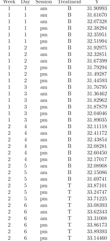
The fuel economy raw data set is presented in Table 2.2. The experiment was

conducted in two weeks shown in the first column. Days were numbered as 1, 2, 3 for the first week and 4, 5, 6 for the second week. There were two sessions- morning and afternoon containing three trials each (e.g. BBB or TTT). The response variable Y on a continuous scale represents miles crossed by a vehicle given a unit gallon of fuel.

For simplicity, we assume that the three back-to-back tests in each half-day session have been averaged. We thus have two results per car per day, one from the morning

and one from the afternoon. In Table 2.2 we treat half-day averages from all six

days as single data point and calculate pooled estimates of between and within

day variation. After manipulation, Table2.2 has been summarized in Table2.3 to

study different contrasts and nested models.

The objective is to estimate the mean for each fuel and the difference in means and to find the median, 25th percentile, and 75th percentile of the posterior distribu-tions of base fuel, test fuel, fuel difference, and day to day variance component.

2.5.1.2 Contrast: T-B

We extract data of week 2 from Table 2.3to prepare Table 2.4 and on days 1-3 we

compare fuels B and T combining between day and within day information.

Model

The mixed model (2.9) has been considered to analyze contrast T-B.

Yjkm =α+βj+δk+jkm (2.9)

(43)

Table 2.2: Data before averaging over back-to-back tests

Week Day Session Treatment Y

1 1 am B 31.90993 1 1 am B 31.61670 1 1 am B 32.07328 1 1 pm B 32.38294 1 1 pm B 32.35951 1 1 pm B 32.51994 1 2 am B 31.92975 1 2 am B 32.32851 1 2 am B 31.67399 1 2 pm B 31.79294 1 2 pm B 31.49287 1 2 pm B 31.44593 1 3 am B 31.76795 1 3 am B 31.36462 1 3 am B 31.82962 1 3 pm B 31.87879 1 3 pm B 32.04046 1 3 pm B 31.89035 2 4 am B 32.11118 2 4 am B 32.41172 2 4 am B 32.43854 2 4 pm B 32.08281 2 4 pm B 32.60450 2 4 pm B 32.17017 2 5 am B 32.08908 2 5 am B 32.15086 2 5 am B 31.69741 2 5 pm T 33.87101 2 5 pm T 33.24747 2 5 pm T 33.71225 2 6 am T 33.08393 2 6 am T 33.62343 2 6 am T 33.31008 2 6 pm T 33.86173 2 6 pm T 33.89393 2 6 pm T 33.14460

(44)

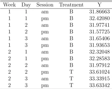
Table 2.3: Data averaged over back-to-back repeats

1 1 am B 31.86663 1 1 pm B 32.42080 1 2 am B 31.97741 1 2 pm B 31.57725 1 3 am B 31.65406 1 3 pm B 31.93653 2 1 am B 32.32048 2 1 pm B 32.28583 2 2 am B 31.97912 2 2 pm T 33.61024 2 3 am T 33.33915 2 3 pm T 33.63342

2) on day k (k = 1, 2, 3) corresponding to the test fuel j (j = 1 or 2) with mean

µjk =E(Yjkm|δk) = α+βj+δk and precision τ = 1/σ2, βj is the fixed effect due

to the jth fuel with the constraint β1 = 0, δk is the day-to-day error term (i.e.

random effects due tokth day) which follows a normal distribution with mean zero

and varianceσ2

b, andjkm is the within-day error term with mean zero and variance

σ2. We can define within-day correlation by ρ = σ2b

σ2

b+σ2

or equivalently ρ = _η₊τ_τ

which can be also be expressed asη = (1−ρ_ρ)×τ, whereη= 1/σ_b2.

Table 2.4: Data to test contrast T-B

2 1 am B 32.32048 2 1 pm B 32.28583 2 2 am B 31.97912 2 2 pm T 33.61024 2 3 am T 33.33915 2 3 pm T 33.63342

We perform Bayesian analysis for the contrast T-B assuming the following priors and using WinBUGS 1.4 (see the Appendix for WinBUGS codes related to this analysis).

(45)

Priors and Results

We assume priors corresponding to model (2.9) as follows

α∼N(38,0.1), βj ∼N(0,0.001)

ρ∼beta(1,1), log(σ)∼U(−20,20)

The prior for α was centered at 38 to incorporate the notion of mean fuel effect

which might hover around 38 as believed by the Shell experimenters. Therefore,

we assume a weakly informative prior for α by taking α ∼ N(38,0.1) and

imple-mented at the beginning. However, Congdon [2007] suggested that, in the absence

of prior information about the direction or magnitude of covariate effects, flat pri-ors may be used by taking univariate normal distributions with mean zero and large variance. The effect of using normal priors with means 0 and large vari-ances is that parameter estimates are smoothed towards zero as large varivari-ances are

used [Galindo-Garre et al.,2004]. Therefore, we tried a non-informative prior forβj

by settingβ2 ∼N(0,0.001) i.e.β2 follows a normal distribution with mean 0 and

lit-tle precision 0.001 or large variance 1000. Also, we assumed a non-informative prior

for σ by assuming log(σ)∼U(−20,20). The prior for the intra-class correlation ρ

is non-informative which is used to compute the precision of the day-to-day error

term. The results are presented in Table2.5assuming the above set of priors.

How-ever, a completely non-informative prior for α, for instance α ∼ N(0,0.001), and

weakly informative prior α∼N(38,0.1) provide similar results to those presented

in Table 2.5 as the concept of non-informative is originated from the assumption

of very little precision.

There were some autocorrelation effects in the results before thinning (where thin-ning refers to removal of some values from the chain). When data were thinned by 15 (i.e. instead of using every step in the chain, we only used every 15th step), then

the autocorrelation disappeared (see also the discussion in Section 2.6). Posterior

means were calculated on the basis of the sample with size 10000. First, 1000 samples were ignored to remove initial fluctuatio