Knowledge Flows and Knowledge Externalities

(1)

K

NOWLEDGE

F

LOWS AND

K

NOWLEDGE

E

XTERNALITIES

G

IOVANNI

P

ERI

CES

IFO

W

ORKING

P

APER

N

O

. 765

C

ATEGORY

5: F

ISCAL

P

OLICY

, M

ACROECONOMICS AND

G

ROWTH

A

UGUST

2002

An electronic version of the paper may be downloaded

• from the SSRN website: www.SSRN.com

(2)

CESifo

Working Paper No. 765

K

NOWLEDGE

F

LOWS AND

K

NOWLEDGE

E

XTERNALITIES

Abstract

The diffusion of knowledge in the world generates positive externalities if

knowledge flows increase the productivity of R&D. Our work analyzes

knowledge diffusion and knowledge externalities in generating innovation and in

determining productivity. We first estimate the determinants of knowledge flows

across 141 sub-national regions in 19 countries of Europe and North America as

revealed by patent citation between US-granted patents. Then we estimate the

impact of these flows on productivity of R&D resources in generating innovation

(patenting) and productivity (TFP). While we find that knowledge diffusion

depends on geographical and technological distance and is well described by a

pseudo-gravity model, we do not find evidence of significant positive externalities

from existing knowledge.

JEL Classification: F0, O3, R1.

Keywords: knowledge flows, innovation, patent citations regions.

Giovanni Peri

Department of Economics

University of California Davis

One Shields Avenue

Davis Ca, 95616

U.S.A.

[email protected]

I thank Shireen Al Azzawi for excellent research assistance. I thank Ryan Brady,

Catherine Guirkinger, Susana Iranzo, Sunhwa Lee, Seungjoon Lee, Melanie

Tauber and Linda Van Diepen for their help with the data and in locating cities in

Europe and North America. I acknowledge the Institue of Governmental Affairs

for partially funding this project. Errors are mine.

(3)

1

Introduction

The concept of Knowledge Externalities has pervasively populated the theo-retical literature on growth for the last ten years. Innovation is the engine of growth, has been argued, and externalities from existing knowledge are the ”re-newable” fuel for this engine. While it is clear how to characterize the source and the effect of these externalities within the frame of a specific model such as Aghion and Howitt [1], Jones [13] or Romer [18], it is much less clear how to measure them in a precise but robust way using the data. First of all it is not clear that there are data that allow us to directly measure such elusive concept as knowledge externalities without adding several other assumptions. Knowl-edge externalities hinge on the diffusion of ideas, a process that leaves no track in the data. Economists have assumed, in order to estimate these externalities, that diffusion of ideas depends on proximity in space, in technological special-ization or in economic development. These are plausible assumptions but each of them is potentially controversial and should be tested. In particular we do not have a good measure of the quantitative dependence of knowledge diffusion on distance or technological proximity. Second, the existence of several effects stemming from the introduction of new ideas, namely their impact on current and future productivity of goods and ideas, has further complicated the task. The goal of this paper is to define clearly, if somewhat narrowly, what knowledge externalities are and use data on patented innovation, citations across patents and total factor productivity to measure the strength of these externalities for 141 sub-national regions covering the whole Western Europe and North Amer-ica.

Knowledge externalities, as all externalities, exist if the social benefit from ideas is larger than the private returns to their inventors. In an economy of competing innovators the private return from an idea is the value of the patent that it entitles to. Therefore we can assume that the whole private contribution of that idea as enhancer of present and future productivity is captured by the patent’s value. In a competitive market for innovation the innovators are able to extract the surplus generated by that innovation. Nevertheless the total social surplus generated by the new idea includes also the contribution (be it positive or negative) that the new idea brings to future discovery of other ideas. We can think of the stock of knowledge as being a state variable and to new patents as theflow that increases that variable. Three contributions of the new ideas have to be considered in order to measure their aggregate return1_{. First, the} private return from a new idea is the benefit due to increased productivity that the idea generates. Second there is a ”capital gain” from this new idea that is the fact that future cost of producing ideas can change and therefore the value of ”new ideas” may vary over time. Third, there may be an externality of new ideas in the production function of ideas. An increase in the stock of knowledge may change the productivity of R&Dresources in generating new knowledge. While thefirst two contributions are fully reflected in the value of the patent,

(4)

the third being an externality, raises the social productivity of the idea above the value of the patent. Crucially, therefore, externality of knowledge exist if ideas increase the productivity of R&D in generating new ideas.

Defining knowledge externalities as we do above may seem somewhat narrow. We assume that there is an efficient market for innovations, that property rights are well defined and enforced by the patent system. If so, when ideas are used in the production of goods, their surplus is extracted by the innovator via the royalties paid on the patent. The only missing market is the one regulating the use of ideas in generation of ideas: no inventor is compensated for the use of her idea in some subsequent discovery that uses it. Many economists believe that externalities from innovation are much more pervasive than that because not all innovations are codified, those that are codified are often not patented and those that are patented are not always effectively protected. Therefore knowledge ”leaks” and it benefits society beyond the private value of the patent. Some economists ultimately argue that externalities should be inferred from measures of total factor productivity (for instance recently, Ciccone [3] and Keller [16] ). Innovation is an important intermediate passage but only when ideas are transferred into productivity gains we have a link between knowledge externalities and output per capita. As we share this view we analyze in the paper the effect of knowledge spillovers on innovation as well as on productivity. We define externalities as disembodied knowledge spillovers that affect the productivity of R&D in the generation of new ideas. This definition captures very important aspects of knowledge externalities and, while not all-inclusive, it is relevant for at least three reasons. First of all the idea of externalities as knowledge spillovers in the creation of new knowledge is behind most (if not all) the theoretical models of endogenous growth, from Romer [18] to Jones [13] passing through Aghion and Howitt [1] and Grossman and Helpman [7]. The strength of this externality determines the difference between ”endogenous” and ”semi-endogenous” model of growth. In general it regulates the dynamics of in-novation in the long run. Second as we limit our analysis to the most advanced economies (Western Europe and North America) we can assume that the pro-tection of property rights on innovation is, in these countries, at its best in the world, minimizing phenomena of imitation and leakages of the patent sys-tem. Granted that leakages due to insufficient protection of intellectual property rights may exist in developing countries, we assume that the effect of knowledge on new ideas is the main source of spillovers in developed countries. Third, using the above definition of spillovers we are able to use data on patent-to-patent citations in order to track the direction and intensity of these knowledge

flows. If the determinants of non-codified knowledge diﬀusion are similar to the determinants of citations then our analysis can be seen as revealing intensity and direction of other kinds of knowledge ”leakages” as well.

The goal of this paper is to estimate the external contribution of available knowledge in generating new knowledge and productivity across regions. Two distinct pieces should be combined in order to establish if existing ideas have any (positive or negative) external eﬀect in the creation of new ideas. First only existing ideas that are actually used by researchers in their process to achieve

(5)

a new idea can generate an externality. Second, only if the use of these ideas increases the productivity of researchers in generating new ideas we have such externality. Previous existing work (with the notable exception of Caballero and Jaffe [2]) merges or assimilates these two phases. Either some mechanical assumption is made on the availability of ideas across space (as in Coe and Helpman [4] and Keller [16] ) so that only a productivity equation is estimated, or knowledgeflows are simply called knowledge externalities without worrying about their effect on productivity (Jaffe et al.[11] , Jaffe and Trajtenberg [12]). In this paper we explicitly model and estimate the phase of knowledge diffusion and utilization in generating new ideas, and the potential impact of this knowl-edge on the productivity of researchers in generating new ideas or in determining TFP.

We use data on patenting and TFP organized in a cross section of 141 regions in Europe and North America in order to estimate the generation of new ideas or of new productive capacity (TFP) from R&D resources. We use data on citation across inventions patented in the US between 1975 and 1996 to measure the intensity of knowledgeflows in the world. Wefind that knowledgeflows depend on several factors and are well represented using a gravity-like equation. Most importantly geographical and technological proximity and crossing a national border affect the intensity of diffusion of ideas. On the other hand we alsofind thatflow-weighted R&D from other regions has small and not significant effect on the generation of new ideas or in determining regional productivity.

The rest of the paper is organized as follows: Section 2 describes the equa-tions that models knowledgeflows and the production function of ideas. Section 3 defines the alternative measures of regional productivity and describes the ac-counting method used to calculate them. Section 4 describes the data we use to measure innovation, productivity, inputs of innovation and theflows of knowl-edge across regions. Section 5 presents the estimates of the parameters in the equation that describes knowledgeflows and in the equation that describes their eﬀect on innovation and productivity. Section 6 concludes the paper.

2

The Model

Two pieces are needed in order to analyze knowledgeflows and knowledge ex-ternalities across regions. Thefirst is a function modelling the diﬀusion of ideas across regions as function of bilateral regional characteristics. In order to pro-duce externalities, ideas originated in a region must be available in other regions as inputs to innovate over the existing knowledge. The second is an innovation function describing how ideas are generated by researchers using R&D spending and existing ideas available to that particular region. The description of these two equations and their estimate occupy the rest of the paper.

(6)

2.1

Di

ﬀ

usion of Ideas

In order to estimate the relative intensity of diﬀusion of ideas across regions using cross-sectional data we divide the ideas discovered in each region in two groups. A group of ideas, discovered earlier (during the 1977-1991 period in our empirical analysis) that can ”send”flows of knowledge to be used in further discoveries, and a group of ideas discovered later (1992-1996 in the empirical analysis) that can ”receive” theflows and use them to generate new ideas. We can use the citation from the receiving to the sending groups of ideas to infer the intensity offlows. Clearly the receiving ideas also cite ideas discovered before the ”sending” (1977) and also cite each other. Nevertheless if theflows of knowledge across regions are stable over time we can infer their relative intensity looking at the equation described in this section.

We denote with∆Ar the ideas (new knowledge) generated in region r(for

”receiving”) during the later interval of time (1992-1996). We denote with∆As

the ideas (new knowledge) generated in region s (for ”sending”) during the earlier period of time (1977-1991). The intensity of diﬀusion to regionrof the ”average” idea originated in region s is denoted as φ(r, s). This index should capture the intensity of ideasflows between regionsand regionrindependently of the total amount of ideas originated in region sand of the total amount of citations produced by ideas in regionr. Defining asσ(s, r) the number of ideas thatflow from sto rthe index is defined as follows:

φ(r, s) = σ(s, r)/ P

sσ(s, r)

∆As/P_s∆As

(1) The term in the numerator σ(s, r)/P_sσ(s, r) captures the share of ideas coming from regionsin the totalflows of ideas coming into regionr. The term in the denominator∆As/Ps∆As is simply the share of total ”sending” ideas

generated in regions. The intensity of diﬀusion between region s and region

rmeasured byφ(r, s) is therefore a relative measure comparable across region-couples and independent from their size. Keeping the receiving region fixed, this index measures the relativeflows of ideas from each of the sending regions, relative to the amount of innovation generated in each sending region. A value of 1 means that regionrreceives from regionsa share of ideas equal to the share of total ”sending” ideas originating ins. Keeping the sending region fixed the index measures the relative absorption of ideas across receiving regions. Notice that the standardization in the numerator implies that we assume equal total absorptive capacity in each region. This depends from the fact that we cannot extract from citation any interesting information on the absolute ”absorptive capacity” of a region. In brief the index φ(r, s) could be considered as the intensity of diffusion of the representative idea between the two regions. The index will be larger than one if diffusion of the average idea between the two regions is stronger than the average diffusion between regions.

Thinking ofφ(r, s) as the intensity of a flow of ideas, we are interested in modelling it as function of bilateral regional characteristics. In particular we describe it as follows:

(7)

φ(r, s) =δe−γ1(d1)r,s_e−γ2(d2)r,s_e−γ3(d3)r,s_ef(Charr,s) ₍₂₎

δ is a parameter scaling the overall flow of ideas between two regions. We can think of it as changing over time but it is constant in our cross-section. The three exponential functions model the decay of ideas flow with distance in geographical space (d1)r,s, technological space (d2)r,s and innovation space

(d3)r,sbetween the two regions2. The exponential functions in (2) can be derived

as the cross-sectional version of a model of diffusion of ideas in time, similar to the one used in Caballero and Jaffe [2]. In the Appendix A we show the derivation of the exponential format from a diffusion process. Theflow of ideas also depends on a vector of other bilateral characteristics of the two regions,

Char_r,s such as being in the same country, sharing a border, using a common language.

In order to use equation (1) and equation (2) for the empirical analysis we establish the following relations between the unobservable variables in (1) and our observables.

1) We assume that the average ”number of ideas” in a patent, indicated as β_s, might be diﬀerent across regions. A slightly diﬀerent (but observationally equivalent) interpretation of this parameter is that it captures the ”average quality ” of ideas contained in the patents of a region. Namely regions whose patents are more ”important” on average, can be thought as having more ideas per patent or the same amount but better quality of ideas per patent. We call this parameter, in general, the ”intensity of ideas per patent”. This parameter may vary over time only according to a factorµcommon to all regions. Denoting with Ps the total number of ”sending” patents granted to regions in

1977-1992 and withPrthe ”receiving” patents granted to region sin 1992-1996,the

above assumptions are summarized by the following conditions: Ps=∆As/µβs,

Pr=∆Ar/βr).

2) We assume that the number of citations from region r to patents from region s contains information on the flow of ideas between the two regions according to the following formula: c(r, s) =ψ_rσ(s, r)ε(r, s).

c(r, s) the total number of citations from patents of region r to patents of region s. As diﬀerent regions may have diﬀerent average absorption capacity and propensity to cite, we allow for a region-specific term ψ_r that combines these two factors. σ(s, r) is the actualflow of ideas between regions. ε(r, s) is a log-normal random noise due to the fact that not all citations capture the

flow of an ideas as some are added by reviewers. We assume that such noise is randomly distributed across region couples (i.e. not correlated withσ(s, r)) .

Substituting these definitions into equation (1) and into equation (2) and using the fact that the total number of citations from regionr, P_sc(s, r) for the Law of Large numbers can be considered approximately non random and equal to the number of citing patentsPr times the average number of citation

per patentnrwe get the following relation:

2_{The exact measure for these three types of distances will be made clear in the empirical} section.

(8)

φ(r, s) = _Pc(r, s)/ε(r, s) sc(s, r)βsPs/P = c(r, s)/ε(r, s) nrPr(Psβs)/P =δe−γ1(d1)r,s_e−γ2(d2)r,s_e−γ3(d3)r,s_ef(Charr,s) (3) where P =P_sPs. Collecting the observables on the left hand side, taking

logs on both sides of (3) and grouping the constants into one term we have the following estimable equation:

ln µ_c₍_{r, s}₎ PrPs ¶ =a+ln (nr)+ln (βs)−γ1(d1)r,s−γ2(d2)r,s−γ3(d3)r,s+f(Charr,s)+u(r, s) (4) Equation (4) can be seen as a generalized Gravity Equation for knowledge spillovers. It is derived from the framework described above and can be brought to the data. We comment here on its meaning and main features. The fre-quency of citation c_P(r,s)

rPs from ideas of regionrto ideas of regionsdepends on a

”citing region”fixed eﬀect, ln (nr),on a ”cited region”fixed eﬀect, ln (βs),on a

sequence of bilateral characteristics (described above) and onu(r, s) = lnε(r, s) that is a normally distributed random error. While the cited regionfixed effect can be interpreted as the ”average intensity of ideas” in patents of ”sending” regions,the citing regionfixed effect should be controlled for but has no inter-esting interpretation. The equation generalizes the concept used in the gravity equation, popular in trade and migration analysis, that the ”flow” of some vari-ables between two regions depends on some characteristics of the two regions and on the ”distance” between them. The Estimating equation (4) allows us to identify the parametersγ₁, γ₂ γ₃ and the vectorf and therefore to estimate the functionφ(r, s) using definition (2). This function captures the diffusion of ideas between two regions and will be used to construct the stock of used ideas as innovative input in the receiving region.

2.2

The Innovation function and Knowledge Spillovers

Once we identify the strength of knowledge flows φ(r, s) we can estimate the impact of these spillovers on the production of new ideas. Assuming that our regions are on a balanced growth path with common rate of knowledge growth we can separate the contribution to innovation of private inputs such as scientists and R&D resources from the external contribution of ideas in the estimation of the innovation function of a region.

New ideas,∆Arare generated from scientists and researchers in regionrand

from their productivity. Productivity of R&D employees in regionrdepends on two main factors: the amount of resources available to them (such as laborato-ries, research funds, salaries and so on) captured by R&D spending per-worker,

(9)

symbolAAV Ar and∆AAV Ar the cumulated stock and the increase in the stock of

ideas available in regionr,respectively. Ar and∆Ar still denote the stock and

the increase of the stock of ideas generated in regionr.The knowledge available in regionr is given by the knowledge generated anywhere thatflows to region

r , namely: AAV A

r =

P

s∈S

φ(r, s)As where φ(r, s) is the intensity in theflow of

ideas described in the previous section. The production function of innovation is therefore: ∆Ar=f(R&Dr, hr, AAV Ar ) =f Ã R&Dr, hr, X s∈S φ(r, s)As ! (5) We assume that regions are on their balance growth path with a common growth rate of knowledge stock Ar so that: (∆Ar/Ar) = g. We check this

assumption with our data and it turns out to be satisfied. Substituting this condition into equation (5) and taking a log-linear expression for the innovation function we have: ln(∆Ar) =−ln(g) +εRDln(R&Dr) +εhln(hr) +εIln Ã X s∈S φ(r, s)∆As ! (6)

εRD is the elasticity of innovation to the supply of scientists. εhis the

elas-ticity of innovation to the supply of resources per scientists. εI is the elasticity

of innovation to available ideas. We can construct the available knowledge in each region using the estimates of φ(r, s) obtained from the previous section (2.1). Denoting with a hat_bthe variable estimates from equation (4) we have:

ln(Pr) = Intercept−ln(bβr) +εRDln(R&Dr) +εhln(hr) + (7) +εIln Ã X s∈S exp³₋_cγ₁(d1)r,s−cγ1(d2)r,s−cγ3(d3)r,s+fb(Charr,s) ´ b β_sPs ! +νr,s

The dependent variable is the count of receiving patents granted in region

r.The termInterceptcontains all the uninteresting constants. The term ln(bβr)

controls for the average intensity of ideas per patent in region r. Controlling for this term is extremely important if the ”intensity” of ideas per patent is correlated with the total amount of patents generated in a region. ln(R&Dr) is

the log of employed in the R&D sector, ln(hr) is the log of spending in US $

per worker in the R&D sector. The term in brackets is the estimated knowledge available in regionr coming from ideas discovered in the past. It is calculated as the intensity of flows to region r (the exponential term) times the amount

(10)

of ideas generated in each region bβsPs. Finally νr,s is a zero average random

disturbance that captures other determinants of patenting not included in our equation.

In our empirical specification wefirst estimate equation (4) and discuss the intensity and direction of spillovers. We then use the estimates from that equa-tion and the observable characteristics of regions to estimate the impact of these spillovers on innovation in regionrby using (7).To avoid the endogeneity problem due to the fact that the expression in brackets contains Pr itself, we

instrument this variable with a similar one, AAV A

−r obtained including all but

regionrin the calculation of available ideas for regionr. Alternatively we will use R&D resources as instrument forPr.

3

Productivity and Knowledge Spillovers

While the most direct measure of new economically useful ideas, defined above as ∆Ar, is certainly given by the count of patents, economists traditionally

measure technological progress and technological differences using total factor productivity (TFP). Total factor productivity captures differences in labor pro-ductivity not due to differences in the use of capital. At some fundamental level, therefore, innovation has an effect on output per capita only if it is translated into increases in TFP. We can consider the TFP of a region as an alternative measure ofAr, that not only captures patented inventions but all innovations

that make production more eﬃcient. Empirically we estimate an equation iden-tical to (6) where ∆Ar, proportional toAr is simply measured using regional

TFP. We modify cross-country accounting techniques in order to calculate the region-specific total factor productivity (ar) and separate it from the country

TFP, (Ac) that is potentially aﬀected by institutional factors. In the following

sections we briefly describe how we obtain two measures of regional TFP: a narrow and a broad one.

3.1

Cross-Regional Productivity Accounting

We assume a Cobb-Douglas production function at the regional level with con-stant return to scale so that elasticity of income to labor and capital equal the share of income going to each of the two factors. Callingαthe share of income going to labor, so that (1₋α) will be the share going to capital, we assume their value to be equal to 0.66 and 0.33 . As we use regional data we may rely on the within country variation to define total factor productivity, disregarding the (probably large) differences in total factor productivity across countries due to institutional and political features of the economies. The cross- regional diff er-ences in TFP can be more appropriately interpreted as differences in the level of technology used (adopted) there. The disadvantage is that we do not have data on physical capital at the regional level. We may nevertheless recover the contribution of regional TFP to production per worker in one of the following

(11)

two ways. We either assume that physical capital moves across regions in order to equate its real return within a country (narrower definition) or we impose the same capital labor-ratio across regions of the same country (broader defi -nition). The first method produces a lower bound of the region-specific TFP differentials, as it attributes part of the regional production per worker diff er-ences to capital intensity. The second method produces an upper bound of these differentials as it attributes the whole region-specific differentials in output per worker to differences in regional TFP. We will perform both decompositions. To be precise, the first one distinguishes among the following three contributions to differentials in output per worker: 1) Differences in regional capital intensity (capital-labor ratios), 2)Differences in country-specific total factor productiv-ity 3) Differences in region-specific TFP. The second decomposition, on the other hand, distinguishes among the following contributions 1) Differences in country-specific TFP 2) Differences in country-specific capital-output ratios 3) Differences in region-specific TFP.

3.1.1 Narrow TFP definition

Let’s assume that the production function for each regionrcan be written as a Cobb-Douglas

Yr=Acar(Lr)α(Kr)1−α (8)

where Yr is total output , Lr is total labor input, Kr total capital input,

Ac is the average TFP of country c to which the region belongs and ar is a

region-specific TFP factor such that ifar>1 the region has larger total factor

productivity than the country as a whole while if ar < 1 then the region has

lower TFP than the country as a whole. Also we assume that P

r∈c

ln(ar) = 0

which implies that the average log TFP for regions of a country is equal to the aggregate country’s log TFP.αis the elasticity of output to labor that equals the income share of labor. In order to decompose total income in the contribution of each component we assume that within countrycthe return paid to capital is the same in each regionrdue to the mobility of capital. This implies:

∂Yr

∂Kr

= (1₋α)Acar(Lr)α(Kr)−α=rc (9)

Marginal productivity of capital at the country level is also equal to rc.

Denoting withkc = (Kc/Lc) the capital-labor ratio for the country. Equation

(9) implies that we can write total capital in regionras:

Kr=kca

1

α

rLr (10)

Substituting Equation (10) into the production function and re-arranging we obtain the following expression for output per capita in regionr:

(12)

Yr Lr =Ackc1−αa 1 α r (11)

Defining output per workeryr=_LYr_r and taking log of both sides of expression

we obtain a variation of the classic growth accounting equation:

lnyr−(1−α) lnkc= lnAc+

1

αlnar (12) The above notation is helpful to understand how to construct each single component of the equation. The left hand side is obtained as log GDP per worker in the region minus the share of capital times the national capital-labor ratio. To obtain the right hand side we can regress the left hand side on a set of country dummies (standardizing one to 0) and the residuals will measure the region-specific TFP term: _α1lnar.Once we calculate these terms we can re-write

the above equation in the following way, that captures exactly the contribution to regional productivity given by regional capital intensity, national TFP and region-specific TFP:

lnyr= [(1−α) lnkc+

1₋α α lnar]

| {z }

Regional Capital Contribution

− lnAc | {z } Country TFP − lnar |{z} Narrow Region TFP (13)

We call this measure of regional TFP the ”narrow” TFP definition. 3.1.2 Broad TFP definition

The second method assumes simply thatkc =kr, i.e. that the capital labor ratio

in each region is equal to the average capital labor-ratio of a country. Under this condition, we simply divide both sides of equation (8) byLr, we substitute

the condition above and take logs. The decomposition of output per worker results as follows:

lnyr= [(1−α) lnkc]

| {z }

Country Capital Contribution

− lnAc | {z } Country TFP − lnar |{z} Broad Region TFP (14)

Note the similarity of the above decomposition with equation (12). Now, as

kc is assumed constant within countries, the diﬀerentials left after controlling

for country-specific factors, are attributed completely to regional TFP diff eren-tials. Compared to the previous method, it is as if the direct effect of TFP and its indirect effect, caused by larger physical capital in the region, are merged together. As TFP differences are the cause for the existence of both terms in

(13)

the decomposition (13), it makes sense to consider also this second method. We call this measure of regional TFP the ”broad” TFP definition. In the imple-mentation of both of these accounting equations we standardize by the average output per worker, capital per worker and the average national TFP in the US to be 1.

4

The Data

Our data on Patented inventions, their Inventors and Citations between them are taken from the NBER Patent Citation data File described in Jaﬀe et al. [9]. We choose only patents granted between 1975 and 1996 for which citation data are available and we organize them across 141 regions3_{: 51 US states including} D.C., 10 Canadian Provinces and 80 regions in 17 European Countries. The regions chosen for Europe are the Territorial Units used by Eurostat and denoted with the name NUTS1. Patents are assigned to the regions of residence of their

first inventor. As the original NBERfile contains only the name of the city and the zip code of thefirst inventor we mapped each city-zip code into a region with the help of national Maps and Gazetteers. The location of thefirst inventor is highly correlated with the location of the other inventors so that this method gives a careful representation of the distribution of innovation in Europe and North America. Moreover the location of the inventor is much more accurate in order to locate where the invention has been in developed, compared to the location of the headquarters of the assignee company.

In our estimate of knowledge flows we want to be particularly careful. We want to measure knowledge diffused to other regions and available there to be used by others and not track the diffusion of knowledge within a network of companies, potentially located in different regions. While the first flow may generate a pure externality the second simply mirrors the existence of large multinational companies that compensate their department in different regions for providing and diffusing knowledge. Therefore we do not include in the count of citations those done between two patents assigned to the same institutions (university, company or research lab). We call these self-citations and we exclude them from the countc(r, s)4_.

The data on employment in R&D and spending per employee in R&D used are the average for the 1992-1996 period of the number of R&D employees and of dollar spent per employee in each region. The averaging over four years allows us to fill some existing gaps in the regional yearly data and provides a value which is less aﬀected by year to year fluctuations. For European regions the data are from the REGIO dataset, for Switzerland data were provided by the Swiss statistical oﬃce, for the U.S. data are from the NSF and for Canada they

3_{The list of regions and countries they belong to is described in Appendix B}

4_{Interestingly if we estimate the speci}_fi_{cations in table 2 including self citations the coe}_ffi -cient that is mostly affected, increasing by 30%, is the one on the Same Region dummy. This confirms our idea that those citations may be within company transfer of knowledge rather than leakages of it. The other coefficients change very little.

(14)

are from Statcan. Data on employment in R&D is the count of people employed in R&D activities. R&D spending has been converted in current dollars before averaging over the four years. A detailed description of the Data can be found in the Data Appendix.

5

Estimation Results

5.1

Di

ﬀ

usion of Ideas

We first estimate the equation of diﬀusion of the representative idea across regions. We divide patents into citing patents (granted in the 1992-1996 period) and cited patents (granted in the 1975-1992). The total count of patents for the citing regionris denoted as (P9296)rand the total count of patents for the cited

region s is denoted as (P7592)s. To have all non zero observation we add one

citation to all the region-couples5 and one patent to (P9296)r and (P7592)s for

each region. The basic specification that we estimate is like equation (4). We include citing and cited regions specific eﬀects (Dr, Ds) to capture, respectively,

diﬀerent propensity to cite/absorb across regions (nr) and diﬀerent intensity of

ideas of the cited regions’ patents (β_s). In the basic specification we include a linear term in geographical distance, in technological distance and in innovative intensity distance (more on this below) and three dummies: one forrandsbeing the same region (SameR) one for them being in the same country (SameC), and one for them sharing a border (ShareB). The basic estimating equation is : ln µ c(r, s) + 1 ((P9296)r+ 1) ((P7592)r+ 1) ¶ =a+Dr+Ds+ (15)

+γ₁(d1)r,s+γ2(d2)r,s+γ3(d3)r,s+f1(SameR)r,s+f2(SameC)r,s+f3(ShareB)r,s+ur,s

Before discussing the estimation of this equation, let us describe in greater detail the three measures of distance d1, d2 and d3 that we include in the re-gression. (d1)r,s is simply the geographical distance between two regions. It is

measured in thousands of kilometers and calculated as the shortest arc distance on the earth surface between two regions, choosing as location of each region the location of its largest metropolitan area. Technological distance (d2)r,s is

a measure of the diﬀerence in technological specialization of two regions. This measure is based on an index of technological proximityfirst introduced by Jaﬀe [10]. This index is calculated as follows: first we divide the patents granted in each region in six (thirty-six in the more detailed formula) technological groups: 5_{We also estimate in Table 4 the equation restricted only to strictly positive}_c₍_{r, s}₎_._Results are very similar to what obtained using all observations.

(15)

Chemical excluding Drugs, Computers and Communications, Drugs and Medi-cal, Electrical and Electronics, MechaniMedi-cal, Others. For each regionswe con-struct the vector of shares of patents in each groupshs= (shs1, ...shs6).Then for each citing-cited region couple (r, s) we construct the uncentered correlation coeﬃcient between vectorshrandshsas follows:

ρ_r,s= P i(shsi∗shri) pP i(shsi)2Pi(shri)2 (16) The uncentered correlation is also the angular distance between the vectors: two regions with identical specialization have a correlation of one, two with orthogonal specialization have a correlation of zero. The technological distance (d3)r,sis equal to 1−ρr,sand is bounded between 0 and 1. Finally the distance

in innovative intensity (d2)r,smeasures how far two regions are in technological

advancement, rather than technological specialization. It is the difference in absolute value of per capita patents granted in the two regions in the 1975-1992 period. A region at the frontier of technological innovation would have a large value of per capita patents while regions that are technologically lagging behind have low values of the same variable. This distance may affect the intensity of spillovers as a region may be more effective in using technology flowing from another region with similar level of technological advancement rather than from a region that is much more (or much less) technologically developed.

Table 1 Descriptive statistics

Variable Mean Std. Deviation Min Max

Number of region to region citations without self-cit.

75.2 516.7 0 68778

Number of region to region citations without self-cit., same technological sub-class

47.5 327.4 0 29478

Geographical Distancea 4.44 3.22 0 13.70

Technological distance (36 sectors) 0.34 0.19 0.006 1

Innovative Advancement Distanceb 1.38 1.52 0 8.48

Number of patents in Cited region (1975-1992)

6523.2 12924.6 1 96804

Number of Patent in citing region (1992-1996)

21609 6523.2 1 52924

Notes: Citation frequencies are calculated omitting self-citations, i.e. citations between patents whose first

author belong to the same company-institution.. a: Thousands of Kilometers.

(16)

Table 1 reports some summary statistics for the data and for the three mea-sures of distance. Geographical distance range from 0 kilometers, when citing and cited region are the same one, to almost fourteen thousands Kilometers (be-tween the US islands of Hawaii and the Greek Islands of Nisia Aigouu-Kriti). Most of the distances, though, are below 10’000 kilometers, in fact only 2% of distances is above 10’000 Km Technological distance range from 0.006 to 1, and innovative advancement distance range from 0 to 8.48. The average number of region to region citation without self-citation is 47 but the variance is very large and the distribution very skewed with many couples with few citations and few couples with a very large number of citations. Our regression results, though, are very robust to the exclusion of outliers.

Table 2

Dependent Variable: Citation Frequency Between Regions

Dep. Var I II III IV

Distance -0.035* (0.002) -0.027* (0.002) -0.045* (0.004) -0.039* (0.003) Same Region 1.65* (0.07) 1.62* (0.07) 1.58* (0.07) 1.36* (0.07) Same Country 0.23* (0.02) 0.17* (0.02) 0.22* (0.02) 0.21* (0.02) Region sharing Border 0.38*

(0.02) 0.36* (0.02) 0.44* (0.02) 0.30* (0.02) Tech. distance- 6 sectors. -1.16*

(0.07)

-1.16* (0.07)

Tech. distance- 36 sectors. -2.00*

(0.06) Distance in Innovative Advancement -0.29* (0.01) -0.30* (0.01) -0.29* (0.01) -0.28* (0.01) Same Language 0.15* (0.01) 0.14* (0.018) 0.11* (0.01) Both NAFTA -0.28* (0.04) -0.27* (0.05) Both EU12 0.04 (0.023) 0.04* (0.02) 141 Citing Region Fixed

Effects

Yes Yes Yes Yes

141 Citied Region Fixed Effects

Yes Yes Yes Yes

Observations 19881 19881 19881 19881

R2 0.96 0.96 0.96 0.97

Notes: Citation frequencies are calculated omitting self-citations. To all region-couples is added one

citation to avoid zeroes. Heteroskedasticity Robust Std errors in parenthesis. *= significant at 1% confidence level.

Table 2 presents the estimates of equation (15) using OLS with Heteroskedas-ticity robust standard errors. Column I is the basic specification that includes same-region, same-country and sharing-border dummies and 141 citing-region, 141 cited-region dummies. Column II adds a dummy for the same language

(17)

spoken in the two regions, and Column III add a dummy for both region in the E.U. and a dummy for both regions in NAFTA. Finally Column IV uses the Technological distance index calculated using 36 sectors rather than 6.

The coeﬃcients of the three measures of distance are extremely precisely es-timated and very stable across specifications. The eﬀect of geographical distance on knowledgeflow is a decrease of 3-4% per thousand Kilometers travelled. At

five thousands Km about 15-20% less of the initial flow of knowledge arrives. Moreover being in the same region, in the same country or sharing a border have each an extremely strong and positive effect on knowledgeflows. Two re-gions in the same country, for instance have about 20% moreflows of knowledge than two regions with the same characteristics but in two different countries. If the citing and cited regions are the same the intensity offlows is 160% stronger than for two different regions. Although we are controlling for self-citations such strong intensity offlows within the same region may be due to some formal or market mediated relations between inventors who operate near each other. Also sharing a regional border has an extra effect of 40% onflows. This effect may be due in part to the arbitrariness of some regional borders that may cut into some economic units such as metropolitan areas (as New-York and New Jer-sey). Technological distance has also a very strong effect. Using the index based on 36 sectors, increasing the technological distance between two regions of one standard deviation (0.19) implies a fall of almost 40% in knowledgeflow between two regions. Finally also the distance in innovative advancement has a very strong effect on knowledge flows. Increasing such distance by a standard deviation (1.52) would reduceflows by 45%.

Less relevant in determining knowledge flows, but still important, are the other characteristics of sharing the same language (increasesflow by 10%) or belonging to the same custom union. Belonging to the European Union increases

flow between two regions by 4% while belonging to NAFTA seems to have a negative eﬀect of -27%. This is probably due to the fact that US patents, other things being equal, tend to cite European patents more than Canadian patents. The ”generalized gravity equation” does an excellent job in explaining knowledgeflows as evidenced by patent citations. Although we do not want to overemphasize the meaning of theR2_{of our regressions, as we are including 392} dummies, their values is always between 0.97 and 0.98.

5.1.1 Robustness Checks

In spite of controlling for a measure of technological distance and a measure of ”innovative distance” we may still think that part of the eﬀect of geographical distance on knowledgeflows is an artifact due to proximity in sector specializa-tion. As we want to specify correctly the diﬀusion of knowledge we check for this possibility. If two close regions are specialized in similar sub-sectors and similar sub-sectors cite each other the geographical distance may be picking up this ef-fect. In Table 3 we estimate the same specifications as done in table 2 but using only, as citations, those between patents in the same technological sub-category. Citations across categories are eliminated so that no issue of sector-composition

(18)

can affect the results. This amounts to using only one narrowly defined techno-logical category and analyze the citations within it and then pool all categories to estimate common parameters of diffusion within each sector. Remarkably most of the coefficient are very similar to those in Table 2. The coefficient on geographic distance, in particular, does not change at all. Even the coefficient on technological distance, in spite of a decrease in its point estimate, remains large and significant. This suggests that technological distance is an important determinant of knowledge flows, even within technological categories and not only across them.

Table 3

Dependent Variable: Within sub-sector Citation Frequency Between Regions Dep. Var I II III IV

(0.06)

-1.11* (0.06)

Tech. distance- 36 sectors. -1.94* (0.06) Distance in Innovative Advancement -0.29 (0.01) -0.30 (0.01) -0.29 (0.01) -0.29* (0.01) Same Language 013* (0.01) 0.11 (0.01) 0.10* (0.02) Both NAFTA -0.26* (0.05) -0.25* (0.05) Both EU12 0.02* (0.02) 0.01 (0.02) 141 Citing Region Fixed Effects Yes Yes Yes Yes 141 Citied Region Fixed Effects Yes Yes Yes Yes Observations 19881 19881 19881 19881

R2 0.96 0.96 0.96 0.965

Notes: Citation frequencies are calculated omitting self-citations and counting only citations between patents in the same technological sub-category. To all region-couples is added one citation to avoid zeroes. Heteroskedasticity Robust Std errors in parenthesis. *= significant at 1% confidence level.

A second check is done in order to make sure that our results do not depend on the inclusion of region couples with zero citations. In Table 2 we used all

(19)

the regions’ couples to get our estimates, including those couples that had zero citations (we added one to all cells). In table 4 we check that the results are robust to the elimination of the zero citations cells. The same specifications are estimated as in Table 2 (column I and II) or in table 3 (column Ia and IIa) only using the couples of regions with at least one citation between each other. Again the estimates are extremely stable and similar to those in table 2 and 3 revealing that the zero-citations region couples do not have any key information on knowledgeflow that is lost considering only the positive citation couples.

Table 4

Omitting regions with 0 citations

Dep. Var I II Ia IIa

(0.07)

-1.76* (0.07) Tech. distance- 36 sectors. -2.15*

(0.06) -2.19* (0.06) Same Language 0.16* (0.02) 0.16* (0.02) 0.16* (0.02) 0.15* (0.02) Both NAFTA -0.18* (0.04) -0.17* (0.04) -0.17* (0.04) -0.16* (0.04) Both EU12 0.001 (0.02) 0.01* (0.02) 0.006 (0.02) 0.01* (0.02) Distance in Innovative Advancement -0.12* (0.01) -0.12* (0.01) -0.13* (0.01) -0.13* (0.01) 141 Citing Region Fixed Effects Yes Yes Yes Yes 141 Citied Region Fixed Effects Yes Yes Yes Yes Observations 14375 14375 13483 13483

R2 0.97 0.97 0.97 0.97

Notes: Citation frequencies are calculated omitting self-citations, i.e. citations between patents whose first author belong to the same company-institution. I-II include all non-self citations Ia-IIa include only citations within same technological sub-category. Region-couples with zero citations between them are dropped. Heteroskedasticity Robust Std errors in parenthesis. *= significant at 1% confidence level.

5.1.2 Eﬀect of Geographical Distance

The decay of knowledgeflows with distance using patent citations has been the object of important empirical analysis (beginning with Jaﬀe et al.[11] and

(20)

con-tinuing in more recent work). This dependence of knowledgeflows on distance has been often used to justify the concept of localized spillovers. Moreover it is interesting to compare how knowledgeflows differ from tradeflows as distance increases, now that we have a common frame given by the gravity equation. In our estimation we were able to separate the effect due to pure geographical distance from other effects such as technological proximity, crossing a national border, crossing a linguistic border and so on. We find, therefore, a genuine distance effect even in the most immaterial of the flows, the one between an existing idea and a new idea. This is interesting as, given the very low cost of spreading information one could have assumed no effect of distance onflows of ideas. Nevertheless as we quantify this effect we realize that knowledge flows are much less sensitive to distance than tradeflows. First of all we explore if it is appropriate to choose a specification of the decay of knowledgeflows that is linear in distance. This is interesting as the standard trade literature specifies a decay which is linear in the logarithm of distance. Such specification implies that flows decay much faster at low than at large distance. If this is true we would observe a clear convexity of the decay function when we estimate a linear specification.

Figure 1: Decay of citation frequency with distance: different polynomial specifications distance linear quadratic cubic polynomial 0 12.5 .253257 1.24029

Figure 1 represents the comparison of the decay function of knowledge dif-fusion with distance, when we estimate such a decay as linear, quadratic, cubic or polynomial in distance. We impose that the linear decay start at 1 (=100% of the knowledgeflow) at distance zero and we plot the decay between zero and

(21)

12.5 thousands of Kilometers. The linear decay shows that the intensity offlows is reduced by about 50% when we reach the distance of 12’000 Kilometers. The function does not exhibit any global concavity or convexity so that we do not gain much using a quadratic or a cubic (dashed lines). Using the polynomial specification we observe a pattern in which the decay is steeper in thefirst 2000 Km, then a ratherflat portion follows up to 6’000 Km and then a steeper de-cay up to 10’000 Km flattening out after that. If we believe in the details of the polynomial representation, we may speculate on how knowledgeflows are more heavily harmed by the initial thousands kilometers and, after that, they have another significant drop only if we cross the ocean (the average distance Europe-US is about 6’000 Km, and recall that all our observations are in Europe and North America). However, such pattern does not dramatically depart from a linear decay. Overall the linear approximation does not miss much, especially if we consider that no point estimate is perfectly reliable. Figure 2 shows the 95% confidence band for the linear estimate and we see that this band contains the point estimate of the polynomial decay for almost the whole range 0-12.5. All in all the linear decay seem to do a good job in approximating the decrease of knowledgeflow with distance as captured by patent citations.

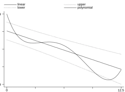
Figure 2: Decay of citation frequency with distance: Linear with 95% confidence band and Polynomial.

distance linear upper lower polynomial 0 12.5 .245289 1.24029

If we compare the eﬀect of distance on knowledge flows with the eﬀect of distance on trade, on the other hand, we find that knowledge flows are gen-uinely much more international. Estimating specification II in table 2 using

(22)

the logarithm of distance (not reported), rather than the level, we can readily compare the effect of distance on inter-regional knowledgeflows with the effect of distance on inter-regional tradeflows, as estimated using Canadian provinces and US states by McCallum [17] . This is one of the few studies using regional trade data that controls for a border effect on top of the distance effect and it is a natural benchmark for our comparison. Our estimate gives a coefficient of -0.14 (std.err. 0.007) as the elasticity of knowledgeflows to distance, while McCallum estimates an elasticity between distance and trade of -1.3 to-1.5. The effects of distance on tradeflows is ten times stronger than the effect of distance on knowledge flows. Incidentally also the border effect estimated by McCal-lum [17](about 3.1) is more than ten times larger than the one we estimate for knowledgeflows (0.23).

5.2

Regions’ Balanced Growth Path

Estimation of Equation (7) is the second task of the paper. That relation relies on the assumption that knowledge growth across regions is on average in Balanced Growth Path during the considered period. In this section we test two important characteristics to make sure that knowledge growth across regions is on BGP with a common long run rate of growth. This, in turn, ensures that Equation (7) is well specified. The two conditions are:

1) (P at9296∗bβ)r=γ(P at7592∗βb)r +er

2) The deviations from the BGP relation written above,er, have zero

aver-age, and are not correlated toR&Dr or hr.

Thefirst condition is the formal implication of the assumption that regions are on BGP growth for their generation of ideas. Assume thatArtis the existing

stock of ideas in regionr and year t and that g is the common yearly growth rate of the stock of ideas in BGP for each regionr. Then considering three years such thatt0< t1< t2 we have, for the generic regioni:

Art2−Art1 = [(1 +g) t2−t1₋_1]_A rt1 (17) Art1−Art0 = [(1 +g) t1−t0₋_1]_A rt0 (18a) Art1 = (1 +g) t1−t0_A rt0 (19)

Merging the three expressions and considering t0 = 75, t1 = 92, t2 = 96 we obtain (Ar96−Ar92) = γ(Ar92−Ar75) where γ = {[(1 +g)4−1](1 + g)17_}/[(1 +g)17₋1].Measuring the change of stock of ideas between two years as the number of patent granted times the estimated intensity of ideas in each patent the equation written above yields: (P at9296∗βb)r = γ(P at7592∗βb)r.

Adding a random disturbance we have the relation under 1).

The second condition ensures that the deviations from BGP, which may be observed, are zero mean, purely random and not correlated with other deter-minants of innovation so that the errors urs in equation (7) are uncorrelated

(23)

with the explanatory variables and estimates of the structural parameters are consistent.

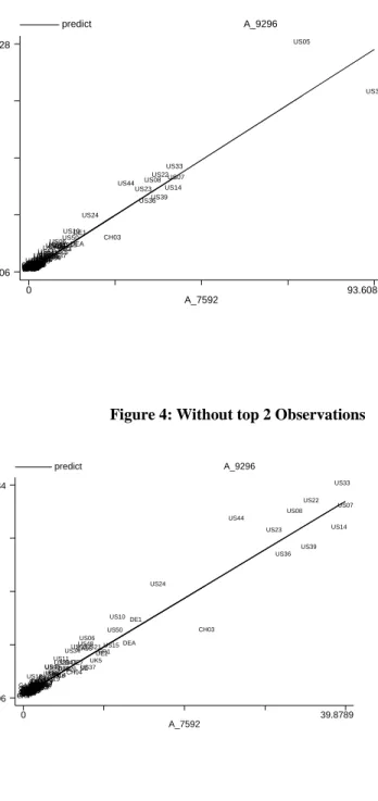
Figure 3: Full Sample 147 Observations

A _9296 A_7592 predict A_9296 0 93.6086 .006 34.1728 AT1 AT2AT3 BE1BE2BE3 CA01 CA02CA03 CA04 CA05 CA06 CA07 CA08CA09CA10 CA11CH02CH01 CH03 CH04 CH05 CH06 CH07 DE1 DE2 DE3 DE4 DE5DE6 DE7 DE8DE9 DEA DEB DEC DED DEEDEF DEGES1ES2ES3ES4ES6ES7ES5DKFI

FR1 FR2 FR3FR6FR4FR5FR8FR7 FR9 GR1GR2 GR3 GR4IEIT1 IT2 IT3 IT4 IT5 IT6 IT7 IT8IT9 ITAITBLU NL1NL2NL3 NL4 NO PT SE UK1 UK2UK3 UK4 UK5 UK6UK7UK8 UK9UKA UKBUS01 US02 US03 US04 US05 US06 US07 US08 US09 US10 US11 US12US13 US14 US15 US16 US17 US18US19 US20 US21 US22 US23 US24 US25 US26 US27US28US29

US30 US31 US32 US33 US34 US35 US36 US37 US38 US39 US40US41 US42 US43 US44 US45 US46 US47 US48 US49 US50 US51

Figure 4: Without top 2 Observations

A_9296 A_7592 predict A_9296 0 39.8789 .006 15.5034 AT1 AT2AT3 BE1 BE2 BE3 CA01 CA02CA03 CA04 CA05 CA06 CA07 CA08 CA09CA10 CA11CH01CH02 CH03 CH04 CH05 CH06 CH07 DE1 DE2 DE3 DE4 DE5DE6 DE7 DE8 DE9 DEA DEB DEC DED DEEDEF DEG DK ES1ES2ES3ES6ES7ES4ES5

FI FR1 FR2 FR3FR6FR5FR4 FR7 FR8 FR9GR1GR3GR2 GR4IE IT1 IT2 IT3 IT4 IT5 IT6 IT7 IT8ITAIT9ITB_LUNL1NL2

NL3 NL4 NO PT SE UK1 UK2UK3 UK4 UK5

UK6_UK7UK8 UK9UKA UKB US01 US02 US03 US04 US06 US07 US08 US09 US10 US11 US12 US13 US14 US15 US16 US17 US18US19 US20 US21 US22 US23 US24 US25 US26 US27US28US29

US30 US32 US33 US34 US35 US36 US37 US38 US39 US40 US41 US42 US43 US44 US45 US46 US47 US48 US49 US50 US51

(24)

Before performing a formal test of condition 1) it is useful to look at Figure 3 and 4. The BGP relation implies that there is a linear relation with zero intercept between the level of ideas generated in regionrduring the period 75-92 (P at9296∗bβ)r and those generated during the period 92-96 (P at7592∗βb)r.

Figures 3 and 4 plot these two variables against each other. Figure 3 incudes all regions while Figure 4 excludes the top two outliers (California and New Jersey) that have many more patents than the other regions. The impression that we get, just from looking at the pictures, is that there exist a very tight linear relation between the two variables and that the intercept of the regression line is just about zero. Table 5, confirms that a linear relation between the two variables explain 95% of the variance of (P at9296∗βb)r and confirms that the

intercept of the linear relation is not statistically diﬀerent from 0 (column I, with all observations and Column III without outliers). Also, no significant concavity or convexity, captured by a quadratic and a cubic term, exists in the relation (Column II and Column IV).

Table 5: Balanced Growth Path relationship

Dep. Val (A_9296)r=(Pat_9296)r*βˆ /1000r

I II III IV

All Observations (146 obs)

Without top 2 outliers (144 obs) Constant -0.18 (0.14) 0.33 (0.17) 0.15 (0.08) -0.11 (0.07) A_7592 0.35* (0.03) 0.22* (0.10) 0.36* (0.02) 0.37* (0.07) (A_7592)2 0.006 (0.005) 0.001 (0.008) (A_7592)3 0.00006 (0.00004) 0.00004 (0.0001) R2 0.95 0.96 0.96 0.96

Table 6 also checks that the residualser from the regression under 1) have

no correlation with R&Dr and hr. Neither in level (Column I) nor in Logs

(Column II) there exist any significant correlation between the residuals and those explanatory variables. These checks, therefore, do not reject our assump-tion that knowledge creaassump-tion in European and North-American regions has been on average on a BGP with a common long run growth rate ofAr. Deviations

from this BGP are rather small, and totally random. In particular they are uncorrelated with regional R&D. As a consequence equation (7) is correctly specified and the level of knowledge generated in each of these regions in the period 1992-1996, depended on the R&D inputs and on the spillovers aﬀecting the ideas generating function.

(25)

Table 6: Independence of Residuals from Explanatory Variables Dep. Var/ Regressors: er ln(er)

R&Dr/1000 0.0023 (0.0047) (hr) 0.074 (0.47) ln(R&Dr) 0.06 (0.05) ln(hr) -0.01 (0.02)

Country Dummies Yes Yes

R2 0.16 0.47

Obs 146 146

Notes: Dep var: er= residuals from regression of A_9296==(Pat_9296)r*exp(βˆr)/1000 on A_7592= =(Pat_7592)r*exp(βˆr)/1000in levels

ln(er)= residuals from a regression as above but in logs

5.3

Innovation Function

We have established, so far, that knowledgeflows across regions depend on sev-eral bilatsev-eral characteristics and notably on distance in geographical, techno-logical and innovative space. Proving the existence of knowledgeflows though, does not prove the existence of externalities (and in particular of positive ex-ternalities) of knowledge in generating innovation unless these flows affect the productivity of researchers in the receiving region. Usage of knowledge origi-nated in other regions may very well bring, together with contribution for new ideas, increased standard of novelty, or a reduction in the ”yet unexplored” in-novation possibilities. These effects may very well generate a zero net effect or even a negative net effect on the productivity of researchers in generating new ideas. Therefore, while no priors are imposed by the theory on the sign and magnitude ofεI,we expect thatεR&Dandεhare positive, as an increase of

re-searchers and of resources should increase theirfindings of new ideas (patented ideas).

We estimate the innovation function in (7). First we construct the stock of available ideas in each regionr,AAV A

r as P s∈S exp³₋_bγ₁(d1)r,s−γb2(d2)r,s−γ3(d3)r,s+fb(Charr,s) ´ b β_sPs

. We use the parameter estimates from Table 2 column I in order to calculate this value. As we have seen those estimates are very robust and precise and therefore it would not make much of a diﬀerence to use the estimates from col-umn II, III or IV. In estimating the equation we include fixed country-eﬀect

Ci, as the propensity to patent in the US may diﬀer across countries, due to

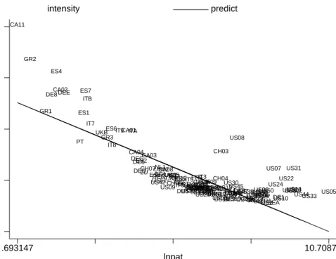
diﬀerent costs and we control also for the previously estimated average intensity of ideas per patent in regions, ln(bβr).Controlling for this variable is important

(26)

ideas per per patent ln(βr) and the patenting intensity ln(Pr) across regions.

Such correlation is represented in Figure 5: regions producing more patents tend to have lower intensity of ideas in each patent.

Figure 5: Intensity of ideas and Patenting intensity across regions

in te n s ity lnpat intensity predict .693147 10.7087 -1.67803 5.96498 AT1 AT2 _AT3 BE1 BE2 BE3 CA01 CA02 CA03 CA04 CA05 CA06 CA07 CA08 CA09 CA10 CA11 CH01 CH02 CH03 CH04 CH05 CH06 CH07 DE1 DE2 DE3 DE4 DE5 DE6 DE7 DE8 DE9 DEA DEB DEC DED DEE DEF DEG DK ES1 ES2 ES3 ES4 ES5 ES6 ES7 FI FR1 FR2 FR3 FR4 FR5 FR6 FR7 FR8 GR1 GR2 GR3 IE IT1 _IT2 IT3 IT4 IT5 IT6 IT7 IT8 IT9 ITA ITB LU NL1 NL2 NL3NL4 NO PT SE UK1

UK2UK4_UK3

UK5 UK6 UK7UK8 UK9 UKA UKB US01 US02 US03 US04 US05 US06 US07 US08 US09 US10 US11 US12 US13 US14 US15 US16 US17 US18US19 US20 US21 US22 US23 US24 US25 US26 US27 US28US29 US30 US31 US32 US33 US34 US35 US36 US37US38 US39 US40 US41 US42 US43 US44 US45 US46 US47 US48 US49 US50 US51

Controlling for ln(β_r) reduces the variability of innovation in response to its inputs. The exact estimated specification is:

ln(Pr) = Ci+cln(bβr) +εRDln(R&Dr) +εhln(hr) + (20)

+εIlnAAV Ar +ur,s

Table 7 reports the estimates of the coeﬃcients of equation (20). The estima-tion method is Instrumental Variables , with Heteroskedasticity robust standard errors. In column I and II the variable

AAV A₋r = X s6=r exp³₋_bγ1(d1)r,s−bγ2(d2)r,s−γ3(d3)r,s+fb(Charr,s) ´ b βsPs

(27)

is used as instrument for AAV Ar , where we have omitted the contribution of

knowledge generated in regionr itself to avoid endogeneity. In column III and IV the variable R&DS_rAV A=X s6=r exp³₋_bγ₁(d1)r,s−bγ2(d2)r,s−γ3(d3)r,s+fb(Charr,s) ´ (R&D_∗h)s

is used as instrument, as our model predicts that resources in R&D are the main exogenous determinant of innovation in a region. In both cases the instru-ment does not include the dependent variable in its calculation and therefore it corrects for the upward bias of the OLS estimation. Column I and III in-cludeR&Dr andhr as separate inputs. Interestingly, though, the elasticity of

innovation are not significantly diﬀerent between these two inputs and we may consider total R&D spending (R&Dr*hr) as a single factor. Doing so (column

II and IV) we obtain a more precise estimate of the elasticity of innovation to this factor. The estimate of such elasticity is around 0.8 with a standard error of 0.07. An increase of R&D resources of 1% increases the generation of new ideas by 0.8% in the long run. Unluckily and diﬀerently from the estimates of εRDandεhthe externalityεI is not estimated precisely. Its standard error is in

fact between 0.4 and 0.5. Nevertheless the point estimate is never significantly diﬀerent from 0 and in column III and IV it is even negative (₋0.5). All in all the evidence point towards large returns of R&D resources in innovation and no positive externalities of knowledge in generating new ideas. In particular if we consider the estimates of column I and II the point estimate ofεI is around

0.1 with standard error of 0.4. We may consider these estimates as potentially biased upward due to the endogeneity of knowledge in the neighboring regions. If we instrumentPs with (R&D∗h)s then we obtain a much smaller and

neg-ative estimate (-0.5) ofεI (column III and IV) still non significantly diﬀerent

from 0. It is possible that a positive ”spillover” of available knowledge is (more than) offset by a negative effect due to increased standard for local innovation brought in the region by the diffusion of outside ideas. Similarly the knowledge and use of existing ideas may very well reduce the space of ”unexplored” ideas, making innovation more difficult.

(28)

Table 7: the production function of innovation Dep. Variableln(Pat_9296)

Dep. Var:ln(Pat_9296) I II III IV

r D R& ) ln( 0.87* (0.12) 0.93* (0.13) r h) ln( 0.65* (0.17) 0.71* (0.18) r h D R& * ) ln( 0.76* (0.067) 0.83* (0.07) AVA r A _0.11 (0.43) 0.12 (0.41) -0.55 (0.50) -0.59 (0.52) r βˆ -0.56* (0.14) -0.55* (0.11) -0.66* (0.12) -0.66 (0.13)

Country Dummies Yes Yes Yes Yes

Observations 141 141 141 141

R2 0.92 0.92 0.91

Notes: Method of estimate: IV with robust std error. Instruments in I, II:      _∑ _∆ ≠r s s A s r ), ( ˆ ln φ or in III and IV      _∑ s s h D R s r,) & * ( ˆ ln φ

5.4

Instrumental Variables: Value of a Patent

Our estimates of the eﬀect of R&D on innovation could be biased up by the presence of some unobservable regional factors , that attract R&D while also increasing its returns in terms of innovation. In order to address this issue we consider a proxy for the value of a patent that varies across regions. If we knew how much a patent were worth in a region, we could explicitly model the fact that researchers are attracted to regions in which patents are more valuable because their expected returns are higher. Moreover if the market value of a patent is independent from the productivity of R&D we could use such variable as an instrument for R&D in regions .

In order to do this, we turn to the idea that a patent is more valuable the largest is the potential market for innovation in the region where it is discovered. Diﬀerent regions have diﬀerent market potentials for innovations, depending on their location and their connections with the other markets. The amount of trade of a region with the rest of the world could reveal the market for the region. More interestingly, though, we have a revealed measure of the potential market for patented goods. This measure is the extent to which patent protection is pursued by resident of a country in other countries. If a patent is protected only on the domestic market it is because the inventors believe that small profits would come by trading the good abroad and therefore it is not worth seeking protection there. On the contrary a patent that is vastly protected reveals the intention of its inventors to protect foreign market and profit on them via trade. Seeking international patenting in other countries reveals what regions the inventor considers as potential markets for the new goods invented there.

(29)

each of our 19 countries to inventors residing in each of them for the period 1993-1996. Identifying the patent protection in a country as the sign that an invention is targeting that country as a market, allows us to estimate the eﬀect of country characteristics and distance on the potential demand for innovations coming from each country. This allows us to calculate the market potential for innovation in each of our regions. We use this measure of market potential as instrument for regional R&D.

Here we briefly describe how we use the data on cross-country patenting to infer the market potential for innovation in each region. Let’s assume that the number πij of patents granted in country j to residents of country i is a

good proxy of the market for new goods that inventions from country i have in country j (in relative terms). We refer to πij as the market for innovation

generated in countryicoming from country j.This seems reasonable as patent protection is a way of ensuring market for new goods.

It is useful to think of the marketπij as depending on countryjand country

i characteristics and on bilateral characteristics aﬀecting the relative intensity of patenting from a country into another. The bilateral characteristic that we use are geographical distance (distij) and a same-country dummy (SameCij).

If we think of πij as the share of total world patents that are granted by

countryj to residents of countryiwe can decompose that value as follows: πij = (Πi,all)(Πall,j)(e−δdistij)(ef SameCij)εij (21)

Πi,all is the share of total patents in the world granted to inventors resident

of countryi, Πall,j is the share of of total patents in the world granted by the

patent oﬃce of countryj. e−δdistij _{is an exponential function in the geographical}

distance betweeniandj, ef SameCij _{is the e}_ﬀ_{ect of patenting in the same country}

where the inventor is resident andεij is a positive multiplicative random factor

distributed as a lognormal that captures all the other bilateral determinants of πij orthogonal to the regressors. As we observeπij anddistij andSameCij we

may use a simple regression to perform the above decomposition. Taking logs of both sides of equation (21) we have:

ln(πij) =Ci+Cj−δ(distij) +f(SameCij) +uij (22)

whereCiandCj are country specific eﬀects and capture the origin and

desti-nation country eﬀects (ln(Πi,all),ln(Πall,j)). distij is the geographical distance

between the two regions andSameCij is a dummy which is equal to one if the

inventor’s country and the granting country are the same. uij= ln(εij) is a zero

mean normally distributed error. Once we have used OLS to estimate equation (22) we can construct the predicted shareπsi,rj which measure the innovation

generated in regionsiof countryiand demanded in regionrjof countryj..While

the parameterCi depends on how innovative is country ithe parametersCj,δ

andf depend only on where inventions are patented and how the distance and national borders aﬀect this marketing decisions. They are therefore variables

(30)

that capture the market potential of a region. Let’s callshmarrj the share of

regionrj in the market for innovation of country j.Also we denote with a hatb

the OLS estimates of our parameters. The predicted potential demand coming from regionrj for innovation invented insi would be:

b

πsi,rj= (shmarrjΠball,j) exp(−δbdistsi,rj+f SameCb sirj) (23)

In our implementation we measureshmarrjas the share of GDP of country

j produced in region rj Therefore the total market potential for innovation

produced in regionsi would be:

P ot1si= X rj X j b πsi,rj (24)

Alternatively, using a region’s gross product as proxy for the demand for new goods (rather thanshmarrjΠball,j) we can define an alternative measure of

demand from regionrj for innovation invented insi:pbsi,rj = exp(−bδdistsi,rj+

b

f SameCsirj)Yrj. The total market potential for regionsi would be:

P ot2si= X rj X j b psi,rj (25)

Both constructs use the geographic position of each region and the inter-country pattern of demand for innovations, revealed by international patenting, to evaluate the main determinant of patent’s value, which is the market potential that a patent has in regionsi once invented.

Table 7b: Instrumenting R&D with Mkt potential Dep. Variable ln(Pat_9296)

Dep. Var:ln(Pat_9296) I II III IV V VI

r h D R& * ) ln( 0.77* (0.04) 0.79* (0.05) 0.77* (0.26) 0.99* (0.19) 0.80* (0.27) 1.01* (0.19) AVA r A -0.52 (0.41) -0.79 (0.59) -0.72 (0.56) r βˆ -0.57* (0.10) -0.52* (0.11) -0.58* (0.22) -0.57* (0.24) -0.55* (0.22) -0.54* (0.23)

Country Dummies Yes Yes Yes Yes Yes Yes

Observations 141 141 141 141 141 141

R2 0.92 0.92 0.89 0.91 0.89

Notes: Method of estimate: Column I and II OLS, Column III and IV, Instrumental variable with robust std

error. Instrumenting ln(R&D*h)rand A AVA

rwith Pot1 and Pot1AVA. Column V and VI use Pot2 and Pot2AVAas instrumental variables.

(31)

Table 7b reports the results of estimating equation (20) using P ot1si or

P ot2siand its transformP otnAV A= P s6=r P s6=r exp³₋_bγ₁(d1)r,s−bγ2(d2)r,s−γ3(d3)r,s+fb(Charr,s) ´ P otn

to instruments for to