Artificial neural networks in bankruptcy prediction: General framework and cross-validation analysis

Theory and Methodology

Arti®cial neural networks in bankruptcy prediction:

General framework and cross-validation analysis

Guoqiang Zhang

, Michael Y. Hu

, B. Eddy Patuwo

, Daniel C. Indro

a_{Department of Decision Sciences, College of Business, Georgia State University, Atlanta, GA 30303, USA} b_{Graduate School of Management, College of Business Administration, Kent State University, Kent, OH 44240-0001, USA}

Received 10 March 1997; accepted 22 December 1997

Abstract

In this paper, we present a general framework for understanding the role of arti®cial neural networks (ANNs) in bankruptcy prediction. We give a comprehensive review of neural network applications in this area and illustrate the link between neural networks and traditional Bayesian classi®cation theory. The method of cross-validation is used to examine the between-sample variation of neural networks for bankruptcy prediction. Based on a matched sample of 220 ®rms, our ®ndings indicate that neural networks are signi®cantly better than logistic regression models in prediction as well as classi®cation rate estimation. In addition, neural networks are robust to sampling variations in overall classi-®cation performance. Ó 1999 Elsevier Science B.V. All rights reserved.

Keywords:Arti®cial intelligence; Neural networks; Bankruptcy prediction; Classi®cation

1. Introduction

Prediction of bankruptcy has long been an important topic and has been studied extensively in the accounting and ®nance literature [2,3, 6,16,29,30]. Since the criterion variable is cate-gorical, bankrupt or nonbankrupt, the problem is one of classi®cation. Thus, discriminant analysis, logit and probit models have been typically used for this purpose. However, the validity and e€ec-tiveness of these conventional statistical methods

depend largely on some restrictive assumptions such as the linearity, normality, independence among predictor variables and a pre-existing functional form relating the criterion variable and predictor variables. These traditional methods work best only when all or most statistical as-sumptions are apt. Recent studies in arti®cial neural networks (ANNs) show that ANNs are powerful tools for pattern recognition and pattern classi®cation due to their nonlinear nonparametric adaptive-learning properties. ANN models have already been used successfully for many ®nancial problems including bankruptcy prediction [62,67]. Many researchers in bankruptcy forecasting including Lacher et al. [33], Sharda and Wilson

*_{Corresponding author. Tel.: 001 330 672 2426; fax: 001 330}

672 2448; e-mail: [email protected].

0377-2217/99/$ ± see front matterÓ1999 Elsevier Science B.V. All rights reserved.

[57], Tam and Kiang [61], and Wilson and Sharda [66] report that neural networks produce signi®-cantly better prediction accuracy than classical statistical techniques. However, why neural net-works give superior classi®cation is not clearly explained in the literature. Particularly, the rela-tionship between neural networks and traditional classi®cation theory is not fully recognized [51]. In this paper, we provide explanation that neural network outputs are estimates of Bayesian poste-rior probabilities which play a very important role in the traditional statistical classi®cation and pat-tern recognition problems.

In using neural networks, the entire available data set is usually randomly divided into a training (in-sample) set and a test (out-of-sample) set. The training set is used for neural network model building and the test set is used to evaluate the predictive capability of the model. While this practice is adopted in many studies, the random division of a sample into training and test sets may introduce bias in model selection and evaluation in that the characteristics of the test may be very di€erent from those of the training. The estimated classi®cation rate can be very di€erent from the true classi®cation rate particularly when small-size samples are involved. For this reason, it is one of the major purposes of this paper to use a cross-validation scheme to accurately describe predictive performance of neural networks. Cross-validation is a resampling technique which uses multiple random training and test subsamples. The advan-tage of cross-validation is that all observations or patterns in the available sample are used for test-ing and most of them are also used for traintest-ing the model. The cross-validation analysis will yield valuable insights on the reliability of the neural networks with respect to sampling variation.

The remainder of the paper will be organized as follows. In Section 2, we give a brief description of neural networks and a general discussion of the Bayesian classi®cation theory. The link between neural networks and the traditional classi®cation theory is also presented. Following that is a survey of the literature in predicting bankruptcy using neural networks. The methodology section con-tains the variable description, the data used and the design of this study. We then discuss the

cross-validation results which will be followed by the ®nal section containing concluding remarks.

2. Neural networks for pattern classi®cation

2.1. Neural networks

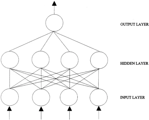
ANNs are ¯exible, nonparametric modeling tools. They can perform any complex function mapping with arbitrarily desired accuracy [14,23± 25]. An ANN is typically composed of several layers of many computing elements called nodes. Each node receives an input signal from other nodes or external inputs and then after processing the signals locally through a transfer function, it outputs a transformed signal to other nodes or ®nal result. ANNs are characterized by the net-work architecture, that is, the number of layers, the number of nodes in each layer and how the nodes are connected. In a popular form of ANN called the multi-layer perceptron (MLP), all nodes and layers are arranged in a feedforward manner. The ®rst or the lowest layer is called the input layer where external information is received. The last or the highest layer is called the output layer where the network produces the model solution. In be-tween, there are one or more hidden layers which are critical for ANNs to identify the complex patterns in the data. All nodes in adjacent layers are connected by acyclic arcs from a lower layer to a higher layer. A multi-layer perceptron with one hidden layer and one output node is shown in Fig. 1. This three-layer MLP is a commonly used ANN structure for two-group classi®cation prob-lems like the bankruptcy prediction. We will focus on this particular type of neural networks throughout the paper.

Like in any statistical model, the parameters (arc weights) of a neural network model need to be estimated before the network can be used for prediction purposes. The process of determining these weights is called training. The training phase is a critical part in the use of neural networks. For classi®cation problems, the network training is a supervised one in that the desired or target re-sponse of the network for each input pattern is always known a priori.

During the training process, patterns or exam-ples are presented to the input layer of a network. The activation values of the input nodes are weighted and accumulated at each node in the hidden layer. The weighted sum is transferred by an appropriate transfer function into the node's activation value. It then becomes an input into the nodes in the output layer. Finally an output value is obtained to match the desired value. The aim of training is to minimize the di€erences between the ANN output values and the known target values for all training patterns.

Let xˆ …x1;x2;. . .;xn† be an n-vector of

pre-dictive or attribute variables,ybe the output from the network,w1andw2 be the matrices of linking

weights from input to hidden layer and from hid-den to output layer, respectively. Then a three-layer MLP is in fact a nonlinear model of the form yˆf2…w2f1…w1x††; …1†

wheref1andf2are the transfer functions for hidden

node and output node, respectively. The most popular choice forf1andf2is the sigmoid function:

f1…x† ˆf2…x† ˆ …1‡eÿx†ÿ1: …2†

The purpose of network training is to estimate the weight matrices in Eq. (1) such that an overall error measure such as the mean squared errors (MSE) or sum of squared errors (SSE) is mini-mized. MSE can be de®ned as

MSEˆ_N1XN jˆ1

…ajÿyj†2; …3†

where aj and yj represent the target value and network output for the jth training pattern re-spectively, and N is the number of training pat-terns.

From this perspective, network training is an unconstrained nonlinear minimization problem. The most popular algorithm for training is the well-known backpropagation [54] which is basi-cally a gradient steepest descent method with a constant step size. Due to problems of slow con-vergence and ineciency with the steepest descent method, many variations of backpropagation have been introduced for training neural networks

[5,13,41]. Recently, Hung and Denton [27] and Subramanian and Hung [59] have proposed to use a general-purpose nonlinear optimizer, GRG2, in training neural networks. The bene®ts of GRG2 have been reported in the literature for many classi®cation problems [35,42,59]. This study uses a GRG2 based system to train neural networks.

For a two-group classi®cation problem, only one output node is needed. The output values from the neural network (the predicted outputs) are used for classi®cation. For example, a pattern is classi®ed into group 1 if the output value is greater than 0.5, and into group 2 otherwise. It has been shown that the least squares estimate as in the neural networks used in this study yields the pos-terior probability of the optimal Bayesian classi®er [51]. In other words, outputs of neural networks are estimates of the Bayesian posterior probabili-ties [28]. As will be discussed in the following section, most classi®cation procedures rely on posterior probabilities to classify observations into groups.

2.2. Neural networks and Bayesian classi®ers

While neural networks have been successfully applied to many classi®cation problems, the rela-tionship between neural networks and the con-ventional classi®cation methods is not fully understood in most applications. In this section, we ®rst give a brief overview of the Bayesian classi®ers. Then the link between neural networks and Bayesian classi®ers is discussed.

Statistical pattern recognition (classi®cation) can be established through Bayesian decision the-ory [15]. In classi®cation problems, a random pattern or observation x2Rn _{is given and then a} decision about its membership is made. Let xbe the state of nature with xˆx1 for group 1 and

xˆx2 for group 2. De®ne

P…xj† ˆprior probability for an observation xbelonging to groupj;

f…xjxj† ˆconditional probability density function forxgiven that the pattern belongs to groupj;

where j ˆ 1, 2. Using Bayes rule, the posterior probability is

P…xjjx† ˆ_f…xjx1†Pf…xj_x1x_{† ‡}j†P…_f…xjxj†_x2†P…x2†;

jˆ1;2: …4†

The Bayes decision rule in classi®cation is a criterion such that the overall misclassi®cation error rate is minimized. The misclassi®cation rate for a givenxis

P…xijx† ˆ1ÿP…xjjx†

ifxbelongs toxj; i;j;ˆ1;2:

Thus, the Bayesian classi®cation rule can be stated as Assignxto groupkif 1ÿP…xkjx† ˆmin_j …1ÿP…xjjx†† or equivalently Assignxto groupkif P…xkjx† ˆmax j P…xjjx†: …5†

It is now clear that the Bayesian classi®cation rule is based on the posterior probabilities. In the case thatf…xjxj†(jˆ1, 2) are all normal distributions, the above Bayesian classi®cation rule leads to the well-known linear or quadratic discriminant function. See [15] for a detailed discussion.

To see the relationship between neural net-works and Bayesian classi®ers, we need the fol-lowing theorem [40].

Theorem 1. Consider the problem of predicting y from x, where x is an n-vector random variable and y is a random variable. The function mapping

F: x!y which minimizes the squared expected

error

E‰yÿF…x†Š2 _6†

is the conditional expectation of y given x,

The result stated in the above theorem is the well-known least-squares estimation theory in statistics.

In classi®cation context, if x is the observed attribute vector and y is the true membership value, that is,yˆ1 if x 2group 1; y ˆ 0 if x 2 group 2, thenF(x) becomes

F…x† ˆE‰yjxŠ ˆ1P…yˆ1jx† ‡0P…yˆ0jx†

ˆP…y ˆ1jx† ˆP…x1jx†: …8† Eq. (8) shows that the least-squares estimate for the mapping function in classi®cation problem is exactly the Bayesian posterior probability.

As mentioned earlier, neural networks are uni-versal function approximators. A neural network in a classi®cation problem can be viewed as a mapping function,F:Rn_{®R(see Eq. (2)), where}

ann-dimensional inputx is submitted to the net-work and a netnet-work outputyis obtained to make the classi®cation decision. If all the data in the entire population are available for training, then Eqs. (3) and (6) are equivalent and the neural networks produce the exact posterior probabilities in theory. In practice, however, training data are almost always a sample from an unknown popu-lation. Thus it is clear that the network output is actually the estimate of posterior probability, i.e.y

estimatesP…x1jx†.

3. Bankruptcy prediction with neural networks

ANNs have been studied extensively as a useful tool in many business applications including bankruptcy prediction. In this section, we present a rather comprehensive review of the literature on the use of ANNs in bankruptcy prediction.

The ®rst attempt to use ANNs to predict bankruptcy is made by Odom and Sharda [38]. In their study, three-layer feedforward networks are used and the results are compared to those of multi-variate discriminant analysis. Using di€erent ratios of bankrupt ®rms to nonbankrupt ®rms in training samples, they test the e€ects of di€erent mixture level on the predictive capability of neural networks and discriminant analysis. Neural net-works are found to be more accurate and robust in both training and test results.

Following [38], a number of studies further in-vestigate the use of ANNs in bankruptcy or busi-ness failure prediction. For example, Rahimian et al. [49] test the same data set used by Odom and Sharda [38] using three neural network paradigms: backpropagation network, Athena and Percep-tron. A number of network training parameters are varied to identify the most ecient training paradigm. The focus of this study is mainly on the improvement in eciency of the backpropagation algorithm. Coleman et al. [12] also report im-proved accuracy over that of Odom and Sharda [38] by using their NeuralWare ADSS system.

Salchenberger et al. [55] present an ANN ap-proach to predicting bankruptcy of savings and loan institutions. Neural networks are found to perform as well as or better than logit models across three di€erent lead times of 6, 12 and 18 months. To test the sensitivity of the network to di€erent cuto€ values in classi®cation decision, they compare the results for the threshold of 0.5 and 0.2. The information is useful when one ex-pects di€erent costs related to Type I and Type II errors.

Tam and Kiang's paper [61] has had a greater impact on the use of ANNs in general business classi®cation problems as well as in the applica-tion of bankruptcy predicapplica-tions. Based on [60], they provide a detailed analysis of the potentials and limitations of neural network classi®ers for busi-ness research. Using bank bankruptcy data, they compare neural network models to statistical methods such as linear discriminant analysis, logistic regression, k nearest neighbor and ma-chine learning method of decision tree. Their re-sults show that neural networks are generally more accurate and robust for evaluating bank status.

Wilson and Sharda [66] and Sharda and Wilson [57] propose to use a rigorous experimental design methodology to test ANNs' e€ectiveness. Three mixture levels of bankrupt and nonbankrupt ®rms for training set composition with three mixture levels for test set composition yield nine di€erent experimental cells. Within each cell, resampling scheme is employed to generate 20 di€erent pairs of training and test samples. The results more convincingly show the advantages of ANNs

rela-tive to discriminant analysis and other statistical methods.

With a very small sample size (18 bankrupt and 18 nonbankrupt ®rms), Fletcher and Goss [19] employ an 18-fold cross-validation method for model selection. Although the training e€ort for building ANNs is much higher, ANNs yield much better model ®tting and prediction results than the logistic regression.

In a large scale study, Altman et al. [4] use over 1000 Italian industrial ®rms to compare the pre-dictive ability of neural network models with that of linear discriminant analysis. Both discriminant analysis and neural networks produce comparable accuracy on holdout samples with discriminant analysis producing slightly better predictions. As discussed in the paper, neural networks have po-tential capabilities for recognizing the health of companies, but the black-box approach of neural networks needs further studies.

Poddig [44] reports the results from an ongoing study of bankruptcy prediction using two types of neural networks. The MLP networks with three di€erent data preprocessing methods give overall better and more consistent results than those of discriminant analysis. The use of an extension of Kohonen's learning vector quantizer, however, does not show the same promising results as the MLP. Kerling [31], in a related study, compares bankruptcy prediction between France and USA. He reports that there is no signi®cant di€erence in the correct classi®cation rates for both American and French companies although di€erent ac-counting rules and ®nancial ratios are employed.

Brockett et al. [10] introduce a neural network model as an early warning system for predicting insurer insolvency. Compared to discriminant analysis and other insurance ratings, neural net-works have better predictability and generaliz-ability, which suggests that neural networks can be a useful early warning system for solvency moni-toring and prediction.

Boritz et al. [9] use the algorithms of back-propagation and optimal estimation theory in training neural networks. The benchmark models by Altman [2] and Ohlson [39] are employed. Re-sults show that the performance of di€erent clas-si®ers depends on the proportions of bankrupt

®rms in the training and testing data sets, the variables used in the models, and the relative cost of Type I and Type II errors. Boritz and Kennedy [8,9] also investigate the e€ectiveness of several types of neural networks for bankruptcy predic-tion problems. Di€erent types of ANNs do have varying e€ects on the levels of Type I and Type II errors. For example, the optimal estimation theory based network has the lowest Type I error level and the highest Type II error level and back-propagation networks have intermediate levels of Type I and II errors while traditional statistical approaches generally have high Type I error and low Type II error levels. They also ®nd that the performance of ANNs is sensitive to the choice of variables and sampling errors.

Kryzanouski and Galler [32] employ the Boltzman machine to evaluate the ®nancial state-ments of 66 Canadian ®rms over seven years. Fourteen ®nancial ratios are used in the analysis. The results indicate that the Boltzman machine is an e€ective tool for neural networks model build-ing. Increasing the training sample size has positive impact on the accuracy of neural networks.

Leshno and Spector [36] evaluate the prediction capability of various ANN models with di€erent data span, neural network architecture and the number of iterations. Their main conclusions are (1) the prediction capability of the model depends on the sample size used for training; (2) di€erent learning techniques have signi®cant e€ects on both model ®tting and test performance; and (3) over-®tting problems are associated with large number of iterations.

Lee et al. [34] propose and compare three hybrid neural network models for bankruptcy prediction. These hybrid models combine statisti-cal techniques such as multi-variate discrimi-nant analysis (MDA) and ID3 method with neural networks or combine two di€erent neural net-works. Using Korean bankruptcy data, they show that the hybrid systems provide signi®cant better predictions than benchmark models of MDA and ID3 and the hybrid model of unsupervised net-work and supervised netnet-work has the best per-formance.

Most studies use the backpropagation algo-rithm [11,38,55,61,64,66] or its variations [43,49] in

training neural networks. It is well known that training algorithms such as the backpropagation have many undesirable features. Piramuthu et al. [43] address the eciency of network training al-gorithms. They ®nd that di€erent algorithms do have e€ects on the performance of ANNs in sev-eral risk classi®cation applications. Coats and Fant [11] and Lacher et al. [33] use a training method called ``Cascade-Correlation'' in a bank-ruptcy prediction analysis. Compared to MDA or Altman's Z score model, ANNs provide signi®-cantly better discriminant ability. Fanning and Cogger [18] compare the performance of a gener-alized adaptive neural network algorithm (GAN-NA) and a backpropagation network. They ®nd that GANNA and backpropagation algorithm are comparable in terms of the predictive capability but GANNA saves them time and e€ort in build-ing an appropriate network structure. Raghupathi [47] conducts an exploratory study to compare eight alternative neural network training algo-rithms in the domains of bankruptcy prediction. He ®nds that the Madaline algorithm is the best in terms of correct classi®cations. However, com-paring the Madaline with the discriminant analysis model shows no signi®cant advantage of one over the other. Lenard et al. [35] ®rst apply the gener-alized reduced gradient (GRG2) optimizer for neural network training in an auditor's going concern assessment decision model. Using GRG2 trained neural networks results in better perfor-mance in terms of classi®cation rates than using backpropagation-based networks.

Based on the pioneering work by Altman [2], most researchers simply use the same set of ®ve predictor variables as in Altman's original model [11,33,38,49,57,66]. These ®nancial ratios are (1) working capital/total assets; (2) retained earnings/ total assets; (3) earnings before interest and taxes/ total assets; (4) market value equity/book value of total debt; (5) sales/total assets. Other predictor variables are also employed. For example, Rag-hupathi et al. [48] use 13 ®nancial ratios previously used successfully in other bankruptcy prediction studies. Salchengerger et al. [55] initially select 29 variables and perform stepwise regression to de-termine the ®nal ®ve predictors used in neural networks. Tam and Kiang [61] choose 19 ®nancial

variables in their study. Piramuthu et al. [43] use 12 continuous variables and three nominal vari-ables. Alici [1] employs two sets of ®nancial ratios. The ®rst set of 28 ratios is suggested by pro®le analysis while the second set of nine variables is obtained by using principal component analysis. Boritz and Kennedy [9] test the neural networks with Ohlson's nine and 11 variables as well as Altman's ®ve variables. Rudorfer [53] selects ®ve ®nancial ratios from a company's balance sheet. It is interesting to note that in the literature one study uses as many as 41 independent variables [36] while Fletcher and Goss [19] and Fanning and Cogger [18] use only three variables.

In order to detect maximal di€erence between bankrupt and nonbankrupt ®rms, many studies employ matched samples based on some common characteristics in their data collection process. Characteristics used for this purpose include asset or capital size and sales [19,36,63], industry cate-gory or economic sector [48], geographic location [55], number of branches, age, and charter status [61]. This sample selection procedure implies that sample mixture ratio of bankrupt to nonbankrupt ®rms is 50% to 50%.

Most researchers in bankruptcy prediction using neural networks focus on the relative per-formance of neural networks over other classical statistical techniques. While empirical studies show that ANNs produce better results for many classi®cation or prediction problems, they are not always uniformly superior [46]. Bell et al. [7] report disappointing ®ndings in applying neural networks for predicting commercial bank failures. Boritz and Kennedy [9] have found in their study that ANNs perform reasonably well in predicting business failure but their performance is not in any systematic way superior to conventional statistical techniques such as logit and discriminant analysis. As the authors discussed that there are many fac-tors which can a€ect the performance of ANNs. Factors in the ANN model building process such as network topology, training method and data transformation are well known. On top of these ANN related factors, other data related factors include the choice of predictor variables, sample size and mixture proportion. It should be pointed out that in most studies, commercial neural

net-work packages are used, which do restrict the users from obtaining a clear understanding of the sen-sitivity of solutions with respect to initial starting conditions.

4. Design of the study

ANNs are used to study the relationship be-tween the likelihood of bankruptcy and the rele-vant ®nancial ratios. Two important questions need to be addressed:

· What is the appropriate neural network archi-tecture for a particular data set?

· How robust the neural network performance is in predicting bankruptcy in terms of sampling variability?

For the ®rst question, there are no de®nite rules to follow since the choice of architecture also depends on the classi®cation objective. For example, if the objective is to classify a given set of objects as well as possible, then a larger network may be desir-able. On the other hand, if the network is to be used to predict the classi®cation of unseen objects, then a larger network is not necessarily better. For the second question, we employ a ®vefold cross-validation approach to investigate the robustness of the neural networks in bankruptcy prediction. This section will ®rst de®ne variables and the data used in this study. Then a detailed description of the issues in our neural network model building is given. Finally, we illustrate cross-validation methodology used in the study.

4.1. Measures and sample

As described in the previous section, most neural network applications to bankruptcy prob-lems employ the ®ve variables used by Altman [2] and often a few other variables are also injected into the model. This study utilizes a total of six variables. The ®rst ®ve are the same as those in Altman's study ± working capital/total assets, re-tained earnings/total assets, earnings before inte-rest and tax/total assets, market value of equity/ total debt, and sales/total assets. The sixth vari-able, current assets/current liabilities, measures the

ability of a ®rm in using liquid assets to cover short term obligations. This ratio is believed to have a signi®cant in¯uence on the likelihood of a ®rm's ®ling for bankruptcy.

A sample of manufacturing ®rms that have ®led for bankruptcy from 1980 through 1991 is selected from the pool of publicly traded ®rms in the United States on New York, American and NASDAQ exchanges. These cuto€ dates for the 12 year sample period ensure that the provisions of the 1978 Bankruptcy Reform Act have been fully implemented and that the disposition of all bank-rupt ®rms in the sample can be established by the 1994 year end. An extensive search of bankrupt ®rms is made of the list provided by the Oce of the General Counsel of the Security Exchange Commission (SEC) and non-SEC sources such as the Wall Street Journal Index and the Commerce House's Capital Changes Reporter as well as the COMPUSTAT research tapes. Company descrip-tions and characteristics required for the identi®-cation of ®ling dates are obtained from LEXIS/ NEXIS news reports as well as other SEC ®lings. The initial search has netted a sample of 396 manufacturing ®rms that have ®led for bankrupt-cy. The following editing procedures are further implemented to remove sources of confounding in the sample. Firms that (1) have operated in a regulated industry; (2) are foreign based and traded publicly in the US; and (3) have ®led bankruptcy previously are excluded from the sample. These sample screenings result in a total of 110 bankrupt manufacturing ®rms.

In order to highlight the e€ects of key ®nancial characteristics on the likelihood that a ®rm may go bankrupt, a matched sample of non-bankrupt ®rms is selected. Financial information for the three years immediately preceding bankruptcy is obtained from the COMPUSTAT database. Non-bankrupt ®rms are selected to match with the 110 bankrupt ®rms in our sample on two key charac-teristics: two-digit Standard Industrial Classi®ca-tion code and size. Size corresponds to the total assets of a bankrupt ®rm in the ®rst of the three years before bankruptcy ®ling. The six ®nancial ratios for the year immediately before the ®ling of bankruptcy are constructed as independent vari-ables in this study. In summary, we obtained a

matched sample of 220 ®rms with 110 observations each in the bankrupt and nonbankrupt group.

4.2. Design of neural network model

Currently there are no systematic principles to guide the design of a neural network model for a particular classi®cation problem although heuris-tic methods such as the pruning algorithm [50], the polynomial time algorithm [52], and the network information technique [65] have been proposed. Since many factors such as hidden layers, hidden nodes, data normalization and training method-ology can a€ect the performance of neural net-works, the best network architecture is typically chosen through experiments. In this sense, neural network design is more an art than a science.

ANNs are characterized by their architectures. Network architecture refers to the number of lay-ers, nodes in each layer and the number of arcs. Based on the results from [14,23,37,42], networks with one hidden layer is generally sucient for

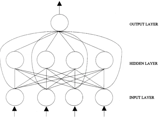
most problems including classi®cation. All net-works used in this study will have one hidden layer. For classi®cation problems, the number of input nodes is the number of predictor variables which can be speci®ed by the particular applica-tion. For example, in our bankruptcy prediction model, the networks will have six input nodes in the ®rst layer corresponding to six predictor vari-ables. Node biases will be used in the output nodes and logistic activation function will be speci®ed in the networks. In order to attain greater ¯exibility in modeling a variety of functional forms, direct connections from the input layer to the output layer will be added (see Fig. 2).

The number of hidden nodes is not easy to determine a priori. Although there are several rules of thumb suggested for determining the number of hidden nodes, such as using n/2, n, n + 1 and 2n + 1 wherenis the number of input nodes, none of them works well for all situations. Determining the appropriate number of hidden nodes usually involves lengthy experimentation since this pa-rameter is problem and/or data dependent. Huang

and Lippmann [26] point out that the number of hidden nodes to use depends on the complexity of the problem at hand. More hidden nodes are called for in complex problems. The issue of the number of hidden nodes also depends on the ob-jective of classi®cation. If the obob-jective is to clas-sify a given set of observations in the training sample as well as possible, a larger network may be desirable. On the other hand, if the network is used to predict classi®cation of unseen objects in the test sample, then a larger network is not neces-sarily appropriate [42]. To see the e€ect of hidden nodes on the performance of neural network classi®ers, we use 15 di€erent levels of hidden nodes ranging from 1 to 15 in this study.

Another issue in neural networks is the scaling of the variables before training. This so-called data preprocessing is claimed by some authors to be bene®cial for the training of the network. Based on our experience (Shanker et al. [56] and also a preliminary study for this project), data transfor-mation is not very helpful for the classi®cation task. Raw data are hence used without any data manipulation.

As discussed earlier, neural network training is essentially a nonlinear nonconvex minimization problem and mathematically speaking, global solutions cannot be guaranteed. Although our GRG2 based training system is more ecient than the backpropagation algorithm [27], it cannot completely eliminate the possibility of encounter-ing local minima. To decrease the likelihood of being trapped in bad local minima, we train each neural network 50 times by using 50 sets of ran-domly selected initial weights and the best solution of weights among the 50 runs is retained for a particular network architecture.

4.3. Cross-validation

The cross-validation methodology is employed to examine the neural network performance in bankruptcy prediction in terms of sampling vari-ation. Cross-validation is a useful statistical tech-nique to determine the robustness of a model. One simple use of the cross-validation idea is consisted of randomly splitting a sample into two

subsam-ples of training and test sets. The training sample is used for model ®tting and/or parameter estimation and the predictive e€ectiveness of the ®tted model is evaluated using the test sample. Because the best model is tailored to ®tone subsample, it often es-timates the true error rate overly optimistically [17]. This problem can be eased by using the so-called ®vefold cross-validation, that is, carrying out the simple cross-validation ®ve times. A good introduction to ideas and methods of cross-vali-dation can be found in [20,58].

Two cross-validation schemes will be imple-mented. First, as in most neural networks classi-®cation problems, arc weights from the training sample will be applied to patterns in the test sample. In this study, a ®vefold cross-validation is used. We split the total sample into ®ve equal and mutually exclusive portions. Training will be con-ducted on any four of the ®ve portions. Testing will then be performed on the remaining part. As a result, ®ve overlapping training samples are con-structed and testing is also performed ®ve times. The average test classi®cation rate over all ®ve partitions is a good indicator for the out-of-sample performance of a classi®er. Second, to have a better picture of the predictive capability of the classi®er for the unknown population, we also test each case using the whole data set. The idea behind this scheme is that the total sample should be more representative of the population than a small test set which is only one ®fth of the whole data set. In addition, when the whole data set is employed as the test sample, sampling variation in the testing environment is completely eliminated since the same sample is tested ®ve di€erent times. The variability across ®ve test results re¯ects only the e€ect of training samples.

The results from neural networks will be com-pared to those of logistic regression. We choose this technique because it has been shown that the logistic regression is often preferred over discrim-inant analysis in practice [22,45]. Furthermore, the statistical property of logistic regression is well understood. We would like to know which method gives better estimates of the posterior probabili-ties and hence leads to better classi®cation results. Since logistic regression is a special case of the neural network without hidden nodes, it is

expected in theory that ANNs will produce more accurate estimates than logistic regression partic-ularly in the training sample. Logistic regression is implemented using SAS procedure LOGISTIC.

5. Results

Table 1 gives the results for the e€ect of hidden nodes on overall classi®cation performance for both training and small test sets across ®ve sub-samples. In general, as expected, one can see when the number of hidden nodes increases, the overall classi®cation rate in the training sets increases. This shows the neural network powerful capability of approximating any function as more hidden nodes are used. However, as more hidden nodes are added, the neural network becomes more complex which may cause the network to learn noises or idiosyncrasies in addition to the under-lying rules or patterns. This is recognized as the notorious model over®tting or overspeci®cation problem [21]. For neural networks, obtaining a model that ®ts the training sample very well is relatively easy if we increase the complexity of a network by, for example, increasing the number of hidden nodes. However, such a large network may have poor generalization capability, that is, it re-sponds incorrectly to other patterns not used in the training process. It is not easy to know a priori when over®tting occurs. One practical way to see this is through the test samples. From Table 1, the best predictive results in test samples are not nec-essarily those with the larger number of hidden nodes. In fact, neural classi®ers with nine or 10 hidden nodes produce the highest classi®cation rates in test samples except for subsample 4 where the best test performance is achieved at four hid-den nodes.

For small test sets, cross-validation results on the predictive performance for both neural net-work models and logistic regression are given in Table 2. This table shows that the overall classi®cation rates of neural networks are con-sistently higher than those of logistic regression. In addition, neural networks seem to be as robust as logistic regression in predicting the overall classi-®cation rate. Across the ®ve small test subsamples,

overall classi®cation rate of neural networks ranges from 77.27% to 84.09% while logistic re-gression yields classi®cation rates ranging from 75% to 81.82%. However, for each category of bankruptcy and nonbankruptcy, the results indi-cate no clear patterns. For some subsamples, neural networks predict much better than logistic regression. For others, logistic regression is better. Table 3 gives the pairwise comparison for these two methods in prediction performance. Overall, neural networks are better than logistic regres-sion and the di€erence of 2.28% is statistically signi®cant at 5% level (p-value is 0.0342). For bankruptcy prediction, neural networks give an average of 81.82% over the ®ve subsamples, higher than 78.18% achieved by logistic regression. For nonbankruptcy prediction, average neural net-work classi®cation rate is 76.09%, lower than av-erage logistic regression classi®cation rate of 78.18%. Paired t-test results show that the di€er-ence between ANNs and logistic regression is not signi®cant in the prediction of bankrupt and nonbankrupt ®rms.

Tables 4 and 5 show the superiority of ANNs over logistic regression in estimating the true classi®cation rate for the large test set. As we have indicated previously, the large test set is basically the available whole sample data which is consisted of a small test sample and a training sample. Hence, the correct classi®cation rates in Table 4 for the large test set are derived directly from the results for both small test sample and training sample. For example, for training sample 1, the total number of correctly classi®ed ®rms in the large test set is 191 which is equal to the best small test result (35) plus the corresponding training result (156).

For large test set, ANNs provide consistently not only higher overall classi®cation rates but also higher classi®cation rates for each category of bankrupt and nonbankrupt ®rms across ®ve training samples. Furthermore, ANNs are more robust than logistic regression in estimating the overall classi®cation rate across ®ve training samples. This is evidenced from the overall clas-si®cation rate of 86.82% for each of the subsam-ples 1, 2 and 5, 87.73% for subsample 3, and 85% for subsample 4. Results of pairedt-test in Table 5

Table 2 Cross-validatio n results on the predictive perf ormance for small test set a Meth od Subs ample 1 b Su bsample 2 Subs ample 3 Subs ample 4 Subsam ple 5 B NB Overall B NB Ove rall B NB Overall B NB Ove rall B NB Ove rall Neural network 15 20 35 20 16 36 20 17 37 18 17 35 17 17 34 (68.18 ) (90.91 ) (79.55 ) (90.91 ) (72.73 ) (81.82 ) (90.91 ) (77.27 ) (84.09 ) (81.82 ) (77.27 ) (79.55 ) (77.27 ) (77.27) (7 7.27) Logistic regress ion 18 16 34 17 17 34 17 19 36 18 17 35 16 17 33 (81.82 ) (72.73 ) (77.27 ) (77.27 ) (77.27 ) (77.27 ) (77.27 ) (86.36 ) (81.82 ) (81.82 ) (77.27 ) (79.55 ) (72.73 ) (77.27) (7 5.00) aThe numbe r in the ta ble is the numbe r of correc tly clas si®ed; percenta ge is given in bra cket. bB stands for bank ruptcy group ;NB stand s for nonban kruptcy gro up. Table 1 The e€ect of hidden nodes on overall clas si®catio n results for tr aining and sma ll test sets a Hidden nodes Su bsample 1 Subs ample 2 Subsam ple 3 Subs ample 4 Subs ample 5 Tra ining b Test c Trainin g Test Training Te st Tra ining Test Trainin g Test 1 139 (78.98 ) 31 (70.46 ) 143 (81.25 ) 36 (81.82 ) 142 (80.68) 37 (8 4.09) 145 (82.39 ) 31 (70.46 ) 142 (80.68 ) 31 (70.46 ) 2 154 (87.50 ) 28 (63.64 ) 143 (81.25 ) 36 (81.82 ) 142 (80.68) 35 (7 9.55) 147 (83.52 ) 34 (77.27 ) 145 (82.39 ) 30 (68.18 ) 3 150 (85.23 ) 27 (61.36 ) 146 (82.96 ) 33 (75.00 ) 142 (80.68) 37 (8 4.09) 151 (85.80 ) 34 (77.27 ) 143 (81.25 ) 30 (68.18 ) 4 148 (84.09 ) 26 (59.09 ) 144 (81.82 ) 27 (61.36 ) 147 (83.52) 35 (7 9.55) 152 (86.36 ) 35 (79.55 ) 153 (86.93 ) 32 (72.73 ) 5 147 (83.52 ) 29 (65.91 ) 145 (82.39 ) 31 (70.46 ) 146 (82.96) 36 (8 1.82) 147 (83.52 ) 32 (72.73 ) 146 (82.96 ) 33 (75.00 ) 6 154 (87.50 ) 31 (70.46 ) 154 (87.50 ) 32 (72.73 ) 153 (86.93) 37 (8 4.09) 154 (87.50 ) 33 (75.00 ) 154 (87.50 ) 31 (70.46 ) 7 156 (88.64 ) 33 (75.00 ) 155 (88.07 ) 35 (79.55 ) 152 (86.36) 37 (8 4.09) 154 (87.50 ) 33 (75.00 ) 154 (87.50 ) 31 (70.46 ) 8 156 (88.64 ) 29 (65.91 ) 156 (88.64 ) 30 (68.18 ) 153 (86.93) 36 (8 1.82) 155 (88.07 ) 28 (63.64 ) 153 (86.93 ) 33 (75.00 ) 9 156 (88.64 ) 35 (79.55 ) 155 (88.07 ) 36 (81.82 ) 156 (88.64) 35 (7 9.55) 156 (88.64 ) 33 (75.00 ) 156 (88.64 ) 32 (72.73 ) 10 158 (89.77 ) 26 (59.09 ) 157 (89.21 ) 31 (70.46 ) 156 (88.64) 37 (8 4.09) 156 (88.64 ) 29 (65.91 ) 157 (89.21 ) 34 (77.27 ) 11 159 (90.34 ) 24 (54.55 ) 158 (89.77 ) 35 (79.55 ) 157 (89.21) 35 (7 9.55) 156 (88.64 ) 30 (68.18 ) 157 (89.21 ) 29 (65.91 ) 12 159 (90.34 ) 27 (61.36 ) 159 (90.34 ) 35 (79.55 ) 156 (88.64) 34 (7 7.27) 159 (90.34 ) 32 (72.73 ) 155 (88.07 ) 34 (77.27 ) 13 159 (90.34 ) 23 (52.27 ) 159 (90.34 ) 26 (59.09 ) 158 (89.77) 34 (7 7.27) 157 (89.21 ) 32 (72.73 ) 158 (89.77 ) 32 (72.73 ) 14 161 (91.48 ) 26 (59.09 ) 159 (90.34 ) 34 (77.27 ) 157 (89.21) 33 (7 5.00) 159 (90.34 ) 31 (70.46 ) 157 (89.21 ) 33 (75.00 ) 15 160 (90.91 ) 29 (65.91 ) 160 (90.91 ) 32 (72.73 ) 159 (90.34) 33 (7 5.00) 160 (90.91 ) 28 (63.64 ) 158 (89.77 ) 31 (70.46 ) aThe nu mber in the table is the numbe r of correc tly clas si®ed; percenta ge is given in brack et. bTraining sample size is 176. cTest sample size is 44.

clearly show that the di€erences between ANNs and logistic regression in the overall and individual class classi®cation rates are statistically signi®cant at the 0.05 level. The di€erences in overall, bank-ruptcy and nonbankbank-ruptcy classi®cation rate are 8.36%, 11.27% and 4.91%, respectively.

Comparing the results for small test sets in Table 2 and those for large test sets in Table 4, we make the following two observations. First, the variability in results across the ®ve large test samples is much smaller than that of the small test set. This is to be expected as we pointed out earlier that the large test set is the same for each of the ®ve di€erent training sets and the variability in the test results re¯ects only the di€erence in the training set. Second, the performance of logistic regression models is stable, while the neural net-work performance improves signi®cantly, from small test sets to large test sets. The explanation lies in the fact that neural networks have much better classi®cation rates in the training samples. Tables 6 and 7 list the training results of neural networks and logistic regression. The training re-sults for neural networks are selected according to the best overall classi®cation rate in the small test set. Neural networks perform consistently and signi®cantly better for all cases. The di€erences between ANNs and logistic regression in overall, bankruptcy and nonbankruptcy classi®cation are 9.54%, 13.18% and 5.90%, respectively.

6. Summary and conclusions

Bankruptcy prediction is a class of interesting and important problems. A better understanding of the causes will have tremendous ®nancial and managerial consequences. We have presented a

general framework for understanding the role of neural networks for this problem. While tradi-tional statistical methods work well for some situations, they may fail miserably when the sta-tistical assumptions are not met. ANNs are a promising alternative tool that should be given much consideration when solving real problems like bankruptcy prediction.

The application of neural networks has been reported in many recent studies of bankruptcy prediction. However, the mechanism of neural networks in predicting bankruptcy or in general classi®cation is not well understood. Without a clear understanding of how neural networks op-erate, it will be dicult to reap full potentials of this technique. This paper attempts to bridge the gap between the theoretical development and the real world applications of ANNs.

It has already been theoretically established that outputs from neural networks are estimates of posterior probabilities. Posterior probabilities are important not only for traditional statistical deci-sion theory but also for many managerial decideci-sion problems. Although there are many estimation procedures for posterior probabilities, ANNs is the only known method which estimates posterior probabilities directly when the underlying group population distributions are unknown. Based on the results in this study and [28], neural networks with their ¯exible nonlinear modeling capability do provide more accurate estimates, leading to higher classi®cation rates than other traditional statistical methods. The impact of the number of hidden nodes and other factors in neural network design on the estimation of posterior probabilities is a fruitful area for further research.

This study used a cross-validation technique to evaluate the robustness of neural classi®ers with respect to sampling variation. Model robustness has important managerial implications particularly when the model is used for prediction purposes. A useful model is the one which is robust across dif-ferent samples or time periods. The cross-valida-tion technique provides decision makers with a simple method for examining predictive validity. Two schemes of ®vefold cross-validation method-ology are employed. Results show that neural networks are in general quite robust. It is

encour-Table 3

Pairwise comparison between ANNs and logistic regression for small test set

Statistics Overall Bankrupt Nonbankrupt

ANN Logistic ANN Logistic ANN Logistic

Mean 80.46 78.18 81.82 78.18 76.09 78.18

t-statistic 3.1609 0.7182 0.1963

Table 4 Cros s-validat ion result s on the estimat ion of true classi®cat ion rates for large test set a Meth od Subs ample 1 b Subs ample 2 Subs ample 3 Subs ample 4 Subs ample 5 B NB Ove rall B NB Overall B NB Overall B NB Overall B NB Overall Neura l 95 96 191 98 93 191 102 91 193 94 93 187 97 94 191 netw ork (86.36 ) (87.27 ) (8 6.82) (89.09 ) (84.55 ) (86.82) (92.73 ) (82.73 ) (87.73) (85.45 ) (84.55 ) (85.00 ) (88.18 ) (85.45 ) (86.82 ) Logistic 87 86 173 87 89 176 83 89 172 86 88 174 81 88 169 regress ion (79.09 ) (78.18 ) (7 8.64) (79.09 ) (80.91 ) (80.00) (75.45 ) (80.91 ) (78.18) (78.18 ) (80.00 ) (79.09 ) (73.64 ) (80.00 ) (76.82 ) aThe numbe r in the table is the numb er of co rrectly clas si®ed; perce ntage is give n in bra cket. bB stands for bank ruptcy gro up; NB st ands for nonban krup tcy group. Table 5 Pairwise comparis on betwee n ANNs and logi stic regress ion for large test set Overall Ba nkrupt No nbankru pt Statistic s ANN Lo gistic AN N Logistic AN N Logistic Mean 86.64 78.55 88.36 77.09 84.91 80.00 t -stat istic 10.38 07 5.621 1 4.0737 p -v alue 0.000 5 0.004 9 0.0152 Ta ble 6 Com parison of ANNs vs. logi stic regress ion on training sam ple a Meth od Subs ample 1 b Subs ample 2 Subs ample 3 Subs ample 4 Subs ample 5 B NB Overall B NB Overall B NB Overall B NB Overall B NB Overall Ne ural 80 76 156 78 77 155 82 74 156 76 76 152 80 77 157 netw ork (90.91 ) (86.36 ) (88.64 ) (88.64 ) (87.50 ) (88.07 ) (93.18 ) (84.09 ) (88.64 ) (86.36 ) (86.36 ) (86.36 ) (90.91 ) (87.50 ) (89.20 ) Logist ic 69 70 139 70 72 142 66 70 136 68 71 139 65 71 136 regr ession (78.41 ) (79.55 ) (78.98 ) (79.55 ) (81.82 ) (80.68 ) (75.00 ) (79.55 ) (77.27 ) (77.27 ) (80.68 ) (78.98 ) (73.86 ) (80.68 ) (77.27 ) aThe numb er in the table is the nu mber of correctl y classi®ed ;pe rcentag e is give n in bracket. bB stands for bankrup tcy group; NB stands for nonb ankruptc y group .

aging to note that the variation across samples in training and test classi®cation rates are reasonably small. Much of the variation in results is associated with the number of hidden nodes and initial start-ing seeds. Users of ANNs will be well advised to use a large number of sets of random starting seeds and experiment on the hidden nodes. After the ``optimal'' solution is identi®ed and the appropri-ate number of hidden nodes is selected, the neural classi®ers tend to provide consistent estimates.

We also compared neural networks with logis-tic regression, a well-known statislogis-tical method for classi®cation. Neural networks provide signi®-cantly better estimate of the classi®cation rate for the unknown population as well as for the unseen part of the population. It can be easily argued that the cost of not being able to predict a bankruptcy is much higher than that for a nonbankrupt ®rm. Neural networks in our study clearly show their superiority over logistic regression in the predic-tion of bankrupt ®rms.

References

[1] Y. Alici, Neural networks in corporate failure prediction: The UK experience, in: A.P.N. Refenes, Y. Abu-Mostafa, J. Moody, A. Weigend (Eds.), Neural Networks in Financial Engineering, World Scienti®c, Singapore, 1996, pp. 393±406.

[2] E.L. Altman, Financial ratios, discriminate analysis and the prediction of corporate bankruptcy, Journal of Finance 23 (3) (1968) 589±609.

[3] E.L. Altman, Accounting implications of failure predic-tion models, Journal of Accounting Auditing and Finance (1982) 4±19.

[4] E.I. Altman, G. Marco, F. Varetto, Corporate distress diagnosis: Comparisons using linear discriminant analysis and neural networks (the Italian experience), Journal of Banking and Finance 18 (1994) 505±529.

[5] R. Battiti, First- and second-order methods for learning: Between steepest descent and Newton's method, Neural Computation 4 (2) (1992) 141±166.

[6] W. Beaver, Financial ratios and predictors of failure, Empirical Research in Accounting: Selected Studies (1966) 71±111.

[7] T.B. Bell, G.S. Ribar, J. Verchio, Neural nets vs. Logistic regression: A comparison of each model's ability to predict commercial bank failures, in: Proceedings of the 1990 Deloitte Touche/University of Kansas Symposium on Auditing Problems, 1990, pp. 29±53.

[8] J.E. Boritz, D.B. Kennedy, E€ectiveness of neural network types for prediction of business failure, Expert Systems with Applications 9 (4) (1995) 503±512.

[9] J.E. Boritz, D.B. Kennedy, A. de Miranda e Albuquerque, Predicting corporate failure using a neural network approach, Intelligent Systems in Accounting, Finance and Management 4 (1995) 95±111.

[10] P.L. Brockett, W.W. Cooper, L.L. Golden, U. Pitaktong, A neural network method for obtaining an early warning of insurer insolvency, The Journal of Risk and Insurance 61 (3) (1994) 402±424.

[11] P.K. Coats, L.F. Fant, Recognizing ®nancial distress patterns using a neural network tool, Financial Manage-ment (1993) 142±155.

[12] K.G. Coleman, T.J. Graettinger, W.F. Lawrence, Neural networks for bankruptcy prediction: The power to solve ®nancial problems, AI Review (1991) 48±50.

[13] M.B. Cottrell, Y. Girard, M. Mangeas, C. Muller, Neural modeling for time series: A statistical stepwise method for weight elimination, IEEE Transactions on Neural Net-works 6 (6) (1995) 1355±1364.

[14] G. Cybenko, Approximation by superpositions of a sigmoidal function, Mathematical Control Signals Systems 2 (1989) 303±314.

[15] R.O. Duda, P. Hart, Pattern Classi®cation and Scene Analysis, Wiley, New York, 1973.

[16] R. Edmister, An empirical test of ®nancial ratio analysis for small business failure prediction, Journal of Finance and Quantitative Analysis 7 (1972) 1477± 1493.

[17] B. Efron, G. Gong, A leisurely look at the bootstrap, the jackknife and crossvalidation, American Statistician 37 (1983) 36±48.

[18] K.M. Fanning, K.O. Cogger, A comparative analysis of arti®cial neural networks using ®nancial distress predic-tion, Intelligent Systems in Accounting, Finance and Management 3 (1994) 241±252.

[19] D. Fletcher, E. Goss, Forecasting with neural networks: An application using bankruptcy data, Information and Management 24 (1993) 159±167.

[20] S. Geisser, The predictive reuse method with applications, Journal of the American Statistical Association 70 (1975) 320±328.

[21] S. Geman, E. Bienenstock, R. Dousat, Neural networks and the bias/variance dilemma, Neural Computation 5 (1992) 1±58.

Table 7

Pairwise comparison between ANNs and logistic regression for training sample

Statistics Overall Bankrupt Nonbankrupt

ANN Logistic ANN Logistic ANN Logistic

Mean 88.18 78.64 90.00 76.82 86.36 80.46

t-statistic 9.9623 6.8578 13.8807

[22] F.E. Harreli, K.L. Lee, A comparison of the discriminant analysis and logistic regression under multivariate nor-mality, in: P.K. Sen (Ed.), Biostatistics: Statistics in Bionmedical, Public Health, and Environmental Sciences, North-Holland, Amsterdam, 1985.

[23] K. Hornik, Approximation capabilities of multilayer feedforward networks, Neural Networks 4 (1991) 251±257. [24] K. Hornik, Some new results on neural network

approx-imation, Neural Networks 6 (1993) 1069±1072.

[25] K. Hornik, M. Stinchcombe, H. White, Multilayer feed-forward networks are universal approximators, Neural Networks 2 (1989) 359±366.

[26] W.Y. Huang, R.P. Lippmann, Comparisons between neural net and conventional classi®ers, in: IEEE First International Conference on Neural Networks, vol. IV, San Diego, CA, 1987, pp. 485±493.

[27] M.S. Hung, J.W. Denton, Training neural networks with the GRG2 nonlinear optimizer, European Journal of Operations Research 69 (1993) 83±91.

[28] M.S. Hung, M.Y. Hu, M. Shanker, B.E. Patuwo, Esti-mating posterior probabilities in classi®cation problems with neural networks, International Journal of Computa-tional Intelligence and Organizations 1 (1996) 49±60. [29] C. Johnson, Ratio analysis and the prediction of ®rm

failure, Journal of Finance 25 (1970) 1166±1168. [30] F.L. Jones, Current techniques in bankruptcy prediction,

Journal of Accounting Literature 6 (1987) 131±164. [31] M. Kerling, Corporate distress diagnosis ± An

interna-tional comparison, in: A.P.N. Refenes, Y. Abu-Mostafa, J. Moody, A. Weigend (Eds.), Neural Networks in Financial Engineering, World Scienti®c, Singapore, 1996, pp. 407±422.

[32] L. Kryzanowski, M. Galler, Analysis of small-business ®nancial statements using neural nets, Journal of Ac-counting, Auditing and Finance 10 (1995) 147±172. [33] R.C. Lacher, P.K. Coats, S.C. Sharma, L.F. Fant, A neural

network for classifying the ®nancial health of a ®rm, European Journal of Operations Research 85 (1995) 53±65. [34] K.C. Lee, I. Han, Y. Kwon, Hybrid neural network models for bankruptcy predictions, Decision Support Systems 18 (1996) 63±72.

[35] M.J. Lenard, P. Alam, G.R. Madey, The application of neural networks and a qualitative response model to the auditor's going concern uncertainty decision, Decision Science 26 (2) (1995) 209±226.

[36] M. Leshno, Y. Spector, Neural network prediction anal-ysis: The bankruptcy case, Neurocomputing 10 (1996) 125±147.

[37] R. Lippmann, An introduction to computing with neural nets, IEEE ASSP Magazine 4 (1987) 2±22.

[38] M. Odom, R. Sharda, A neural network model for bankruptcy prediction, in: Proceedings of the IEEE International Conference on Neural Networks, II, 1990, pp. 163±168.

[39] J. Ohlson, Financial ratios and the probabilistic prediction of bankruptcy, Journal of Accounting Research 18 (1) (1980) 109±131.

[40] A. Papoulis, Probability, Random Variables, and Sto-chastic Processes, McGraw-Hill, New York, 1965. [41] D.B. Parker, Optimal algorithm for adaptive networks:

Second order back propagation, second order direct propagation, and second order Hebbian learning, in: Proceedings of IEEE International Conference on Neural Networks, 1987, pp. 593±600.

[42] E. Patuwo, M.Y. Hu, M.S. Hung, Two-group classi®ca-tion using neural networks, Decision Science 24 (4) (1993) 825±845.

[43] S. Piramuthu, M.J. Shaw, J.A. Gentry, A classi®cation approach using multi-layered neural networks, Decision Support Systems 11 (1994) 509±525.

[44] T. Poddig, Bankruptcy prediction: A comparison with discriminant analysis, in: A.P.N. Refenes (Ed.), Neural Networks in the Capital Markets, Wiley, Chichester, 1995, pp. 311±324.

[45] S.J. Press, S. Wilson, Choosing between logistic regression and discriminant analysis, Journal of American Statistical Association 73 (1978) 699±705.

[46] J.R. Quinlan, Comparing connectionist and symbolic learning methods, in: G. Hanson, G. Drastal, R. Rivest (Eds.), Computational Learning Theory and Natural Learning Systems: Constraints and Prospects, MIT Press, Cambridge, MA, 1993.

[47] W. Raghupathi, Comparing neural network learning algorithms in bankruptcy prediction, International Jour-nal of ComputatioJour-nal Intelligence and Organizations 1 (3) (1996) 179±187.

[48] W. Raghupathi, L.L. Schkade, B.S. Raju, A neural network approach to bankruptcy prediction, in: Proceed-ings of the IEEE 24th Annual Hawaii International Conference on Systems Sciences, vol. 4, 1991, pp. 147±155. [49] E. Rahimian, S. Singh, T. Thammachote, R. Virmani, Bankruptcy prediction by neural network, in: R. Trippi, E. Turban (Eds.), Neural Networks in Finance and Investing: Using Arti®cial Intelligence to Improve Real-World Per-formance, Probus, Chicago, IL, 1993, pp. 159±176. [50] R. Reed, Pruning algorithm ± A survey, IEEE

Transac-tions on Neural Networks 4 (5) (1993) 740±747. [51] M.D. Richard, R.P. Lippmann, Neural network classi®ers

estimate Bayesian a posterior probabilities, Neural Com-putation 3 (1991) 461±483.

[52] A. Roy, L.S. Kim, S. Mukhopadhyay, A polynomial time algorithm for the construction and training of a class of multilayer perceptrons, Neural Networks 6 (1993) 535± 545.

[53] G. Rudorfer, Early bankruptcy detection using neural networks, APL Quote Quad 25 (4) (1995) 171±176. [54] D.E. Rumelhart, G.E. Hinton, R.J. Williams, Learning

internal representations by error propagation, in: D.E. Rumelhart, J.L. Williams (Eds.), Parallel Distributed Processing: Explorations in the Microstructure of Cogni-tion, MIT Press, Cambridge, MA, 1986.

[55] L.M. Salchengerger, E.M. Cinar, N.A. Lash, Neural networks: A new tool for predicting thrift failures, Decision Sciences 23 (4) (1992) 899±916.

[56] M. Shanker, M.Y. Hu, M.S. Hung, E€ect of data standardization on neural network training, Omega 24 (4) (1996) 385±397.

[57] R. Sharda, R.L. Wilson, Neural network experiments in business-failure forecasting: Predictive performance measurement issues, International Journal of Compu-tational Intelligence and Organizations 1 (2) (1996) 107±117.

[58] M. Stone, Cross-validatory choice and assessment of statistical predictions, Journal of the Royal Statistical Society B 36 (1974) 111±147.

[59] V. Subramianian, M.S. Hung, A GRG2-based system for training neural networks: Design and computational experience, ORSA Journal on Computing 5 (4) (1993) 386±394.

[60] K.Y. Tam, Neural network models and the prediction of bank bankruptcy, OMEGA 19 (5) (1991) 429±445. [61] K.Y. Tam, M.Y. Kiang, Managerial applications of neural

networks: The case of bank failure predictions, Manage-ment Science 38 (7) (1992) 926±947.

[62] R.R. Trippi, E. Turban, Neural Networks in Finance and Investment: Using Arti®cial Intelligence to Improve Real-World Performance, Probus, Chicago, IL, 1993. [63] J. Tsukuda, S. Baba, Prediction Japanese corporate

bankruptcy in terms of ®nancial data using neural network, Computers and Industrial Engineering 27 (1994) 445±448.

[64] G. Udo, Neural network performance on the bankruptcy classi®cation problem, Computers and Industrial Engi-neering 25 (1993) 377±380.

[65] Z. Wang, C.D. Massimo, M.T. Tham, A.J. Morris, A procedure for determining the topology of multilayer feedforward neural networks, Neural Networks 7 (1994) 291±300.

[66] R.L. Wilson, R. Sharda, Bankruptcy prediction using neural networks, Decision Support Systems 11 (1994) 545± 557.

[67] F. Zahedi, A meta-analysis of ®nancial application of neural networks, International Journal of Computational Intelligence and Organizations 1 (3) (1996) 164±178.