Working Paper Series
WP 2009-20
School of Economic Sciences
Long Term Versus Temporary
Certified Emission Reductions in
Forest Carbon-Sequestration
Programs
By
Gregmar Galinato, Aaron Olanie,
Shinsuke Uchida, and Jonathan
Yoder
Date Revised: June 30, 2010
Long Term Versus Temporary Certified Emission Reductions in Forest
Carbon-Sequestration Programs
Gregmar I. Galinato* School of Economic Sciences Washington State University Pullman, WA 99164 Email: [email protected] Tel: (509) 335-6382 Fax: (509) 335-1173 Aaron Olanie School of Economic Sciences Washington State University Pullman, WA 99164 Email: [email protected] Tel: (509) 335-8600 Fax: (509) 335-1173 Shinsuke Uchida Department of Agricultural and Resource Economics University of Maryland College Park, MD 20740 Email: [email protected] Tel: (301) 405-1293 Fax (301) 314-9091 Jonathan Yoder School of Economic Sciences Washington State University Pullman, WA 99164 Email: [email protected] Tel: (509) 335-8596 Fax: (509) 335-1173 *Contact Author JEL: Q2, Q54, Q23Under the Clean Development Mechanism (CDM) of the Kyoto Protocol, forest projects can receive returns for carbon sequestration via two credit instruments: temporary (tCERs) or long-term certified emission reductions (lCERs). This article develops a theoretical model of optimal harvesting strategies that compares private optimal harvest decision under these two instruments. Risk-neutral, profit maximizing landowners are likely to prefer instituting lCERs over tCERs. A particular type of early harvest penalty implemented under the lCERs is critical in determining the length of rotation intervals and the carbon credit supply. When this penalty is an increasing function of the difference in biomass before and after harvesting across verification periods, the landowner chooses a different rotation interval compared to the Faustmann rotation which may be longer or even shorter. The resulting supply curve may have a backward bending region over a range of carbon prices.
1. Introduction
Given the recent concerns over climate change, various programs and projects have been proposed to mitigate greenhouse gas emissions. Afforestation and reforestation projects have the potential to sequester significant amounts of carbon through transpiration of carbon dioxide and other greenhouse gases (Binkley and Van Kooten 1994; Cacho et al. 2003; Lee et al. 2005; Nordhaus 1991; Richards 1992; Sedjo and Solomon 1989). Under the Clean Development Mechanism (CDM) of the Kyoto Protocol, forest projects can be developed to offset man-made carbon emissions and generate carbon credits as temporary or long-term certified emission reductions; tCERs and lCERs, respectively (UNFCCC 2003).
The tCERs and lCERs are carbon emissions offset credits generated by forest owners who produce forest biomass verified by the CDM executive. These CERs are purchased by users of carbon credits to meet their carbon emissions compliance requirements. The forest owners benefit because they are able to generate extra revenues from standing forest biomass. A unit of tCER is equal to one metric ton of carbon dioxide equivalent (CO2e) sequestered from trees (CDM Rulebook, 2009a). These tCERs are valid for use as carbon offsets by obligated parties during a five-year commitment period, but not after (UNFCCC 2003). After the tCER commitment period is over, the buyers of CO2e offsets must either contract for more tCERs or satisfy their emissions obligations in some other way.
LCERs are credits generated by a forest owner under a contractual arrangement spanning up to 60 years (UNFCCC 2003). Unlike tCERs, lCER accrual is based on incremental additions to biomass between multiple, discrete, verification periods (UNFCCC 2006; CDM Rulebook, 2009b). Accrued lCERs can be used as valid CO2e offsets not only during the commitment period between verification periods, but also for the entire crediting period up to 60 years.
However, if there is a biomass reduction event between verifications (such as harvest), there will be a penalty or reduction in valid accumulated lCERs equal to the reduction in CO2e sequestered.1 If this occurs, obligated parties must satisfy their offset obligations through the additional acquisition of CERs or by some other means. The interaction between sequestration verification and rotation interval choice is important because harvest leads to a reduction in forest biomass. The specifics of these two instruments affect their relative effectiveness and outcomes in terms of carbon sequestration incentives.
Only one forest project was approved by the CDM executive that generated tCERs before 2009, but fourteen more projects were approved by June 2010 (UNFCCC, 2010). More emphasis has been given to understanding the effect of tCERs in forestry projects (Galinato and Uchida, 2010, forthcoming). We are not aware of any study that has modeled the impact of lCERs on harvesting decisions and carbon credit supply.
In light of potential increasing reliance on CERs, this article develops a theoretical model for examining optimal harvesting strategies based on the value of harvested timber and revenues from sequestered carbon under lCERs. We simulate optimal rotation intervals and carbon supply curves under the lCERs instrument using our model and compare it with simulations for tCERs. Comparing both the mechanisms, tCERs and lCERs, which regulate these forestry projects will be a vital tool as they are revised in the future. The theoretical results are applied to Tanzania and the Philippines, two developing countries that have the potential to sponsor afforestation and reforestation projects to generate lCERs under the CDM. The study also provides a dynamic
1
This is a stylistic representation of the harvest penalty based on the current conceptual framework outlined in the modalities and procedures for afforestation and reforestation project activities under CDM (UNFCCC 2003). In practice, the penalty in a project depends on negotiations between the buyer and seller of the credits as well as the
framework for measuring the feasibility of a given forest plantation that sequesters carbon under this instrument.
There are two main disadvantages of the tCERs instrument relative to lCERs. First, tCER offset creation ceases to exist if the host country or landowner decides to default on the project because of the short run implementation of this instrument. Second, because of the shorter term nature of tCERs, they are not as compatible with credits generated from national or regional emissions trading schemes such as the European Union allowance (Bird et al 2004). The lCERs instrument addresses both of these issues to some extent. Even though there is no project yet to date that has been approved using this instrument, it is important to understand the potential implications of such a policy as forest projects are approved and the instrument is refined.
This paper extends a growing literature on carbon sequestration instruments for forestry. Germain, et al. (2007) and Olschewski et al. (2005) examined the economic feasibility of carbon credit projects for developing countries given the new carbon crediting mechanisms for forest projects. However, their model did not consider the dynamic aspects of rotation interval choices and corresponding carbon storage. Integrating a positive value attached to a continuous flow of sequestered carbon dioxide emissions in optimal forest rotation models are likely to result in socially optimal rotation intervals that are longer than the privately selected rotation interval (Plantinga and Birdsey 1994). Several studies have extended the basic model. Hoen and Solberg (1997) and Van Kooten et al. (1995) derive the optimal carbon subsidies / taxes to internalize the carbon sequestration function of the forest. Spring et al. (2005) explain the effect of wildfire risk in sequestering forest carbon. Guthrie and Kumareswaran (2009) also incorporate the effect of carbon credits in rotation interval choice using actual carbon sequestered versus long run sequestration potential of the land in a continuous model.
Galinato and Uchida (forthcoming) were the first to examine the effect of implementing the current tCERs mechanism on the choice of rotation intervals and the supply of carbon credits. Galinato and Uchida (2010) extend the analysis by measuring the effectiveness of the current tCERs framework relative to social welfare and find that the tCERs instrument results in only a 2% lower level of social welfare relative to the social optimum. Our article is the first study that we know of that investigates the effect of lCERs, as outlined in the UNFCCC modalities and procedures for forest activities, on rotation intervals and carbon credit supplies of forestry projects.
The discrete nature of verification periods under the CDM along with the other characteristics of lCERs lead to some idiosyncratic effects on rotation choice and carbon credit supply. Based on our theoretical model, we find that the design and implementation of a penalty under the lCERs is critical in determining both the length of rotation intervals as well carbon credit supply. Given the current guidelines for lCERs, the type of penalty has opposing incentives on rotation length. The penalty is an increasing function of the difference in biomass before and after harvesting between verifications. Thus, the landowner can reduce the nominal value of the penalty by shortening the rotation interval, but he can also reduce the present value by lengthening it. If the former effect is more (less) significant than the latter effect, the rotation interval is shorter (longer).
Increasing the sequestration of carbon is the stated goal of CERs, but the structure of lCER penalties leads to some potentially surprising carbon sequestration outcomes. We show that in some cases there is a backward-bending region in the carbon sequestration supply curve. For some parameterizations, lCERs instruments induce very little increase in carbon sequestration for a given forest stand. However, a higher carbon price increases land rents for
stands under lCER certification, so lCERs provide the incentive for land conversion from other uses to forestry. Taken together, the results of our model have important policy implications especially with regard to carefully designing the penalty and highlight the potential effect of lCERs in afforestation and reforestation projects that adopt such an instrument.
The rest of the paper proceeds as follows: the next section provides an overview of the current guidelines for generating lCERs with afforestation and reforestation programs under the CDM and compares it with tCERs. Section 3 presents the theoretical model for lCERs that solves for optimal rotation intervals under an infinite rotation horizon. Section 4 summarizes results from simulations in the Philippines and Tanzania. Section 5 concludes the study.
2. An Overview of Temporary and Long Term Certified Emission Reductions
Under the CDM, forestry projects that wish to be credited with tCERs or lCERs are subject to a number of participation criteria and technical standards. The host country must have ratified the Kyoto Protocol and established a Designated National Authority (DNA) that determines the feasibility of crediting projects within the country. To be eligible, a proposed forest project must not be required by national or local law, and the targeted land must be without forest cover between December 31, 1989 and the starting date of the project. Under the current rules, tCERs and lCERs forest projects can last from 20 to 60 years depending on the type of trees, other economic policies and environmental factors (UNFCCC 2003).
Figure 1 demonstrates how lCERs are generated under a multiple rotation system for a hypothetical forest project. The landowner chooses the first crediting verification of sequestered carbon at any point after the forest project starts (UNFCCC 2003). After the first verification, the subsequent verification periods take place every five years until the end of the project (UNFCCC 2003). At each verification period, the DNA verifies and issues certified lCERs based upon the
marginal (additional) carbon sequestered from the previous verification period to the current verification period. In the example in Figure 1, the project starts in the year 2010 and the first verification period is chosen by the landowner in year 2012. After the initial verification, verification and issuance of lCERs occurs every five years thereafter, so the next verification periods are 2017, 2022 and so on until the end of the project at year 2032.
LCERs purchased by firms are valid as CO2e offsets through the end of the crediting period (of up to maximum 60 years) and depends on incremental gains (and losses) in biomass. If a landowner sells lCERs early in the crediting period based on expected biomass accumulation but there is a subsequent loss in biomass due to harvesting or any other event, the landowner may be required to replace or remunerate the buyer for this reduction in lCERs (UNFCCC 2003; Bird et al. 2004). Alternatively, the landowner may choose to retire lCERs altogether and not sell them. The landowner can still earn additional revenue from sequestered carbon in subsequent verifications as long as the volume of trees in subsequent verifications is larger than previous verifications.
Projects that adopt tCERs are subject to the same participation criteria and technical standards as lCERs. TCERs are issued every five years following the initial crediting verification. The amount of tCERs generated is based on total amount sequestered in a given verification period. Also, tCERs expire after five years once the subsequent tCER has been issued, thus they are termed “temporary” (UNFCCC 2003). If there is any loss in biomass, there is no penalty since validity of tCERs is not dependent on project length and loss of biomass (UNFCCC 2006). Figure 2 illustrates an example of tCERs. Here, the first verification occurs in year 2012. Thus, subsequent verification periods occur at years 2017, 2022 and 2027. The corresponding amount of carbon credits generated are based on the cumulative amount of carbon
sequestered as shown in the vertical axis on the right hand side. Loss in biomass due to harvesting has no impact on validity of tCERs but can affect the amount of carbon credited in the next verification cycle.
3. Infinite rotation model for Long Term Certified Emission Reductions
We integrate two important characteristics of the lCERs instrument into an optimal rotation model. First, lCERs are based on additional carbon sequestered from one verification period to the next. Second, we account for the loss of any biomass during harvest as a penalty based on the marginal reduction of carbon sequestered between verification periods.2
We suppose that a landowner maximizes the net present value of forest activities by selecting optimal forest rotation intervals in an infinite time horizon for an even-aged stand. We consider timber revenues and certified lCERs as the primary benefits by the landowner where the latter are earned in a 60-year crediting period during the forest project. In an infinite rotation model with lCERs, the rotation intervals can be grouped into two types. The first is the rotations after the 60-year crediting period expires and the second is during the crediting period when lCERs are created by incremental carbon sequestration. We solve the model in two parts by deriving the optimal harvest without carbon credits to derive the value function. Next, we substitute the value function into the main objective function to solve for the rotations during the crediting period.
3.1 Rotations after the carbon crediting period
After the maximum 60-year crediting period, the landowner earns value only from timber. Assuming constant net timber price, discount rate and planting cost, the discounted profit from forest rotations after the crediting period, a, is equal to
2
One alternative option would be to disallow landowners to sell carbon credits based on the amount of reduced sequestered carbon; however, adding in a penalty is equivalent and more expedient mathematically.
( ) max 1 f f v f a rt t p V t Q Q e (1)
where V() is concave volume function of timber, pv is the price of timber net the harvesting cost,
Q is the fixed cost of planting and r is the discount rate.Note that the optimal value a* starts
when the last rotation interval during the 60-year crediting period ends. Thus, a* occurs any
time after year 60 and does not necessarily start in year 61. The optimal rotation interval after the crediting perios is the Faustmann solution, tf, where the marginal value of timber equals the
marginal opportunity cost of timber and land.
3.2 Rotations during the carbon crediting period
During the 60-year crediting period, the landowner earns revenues from timber and the generated lCERs. The number of lCERs generated during each five year period is a function of the additional carbon biomass relative to the previous verification period. Biomass is a function of tree volume and wood density. Because the verification intervals are fixed at five years, the timing of the first verification period relative to forest stand age determines the timing of all other verifications during the 60-year crediting period. During the first forest stand rotation, the present value of carbon revenues, R1, is
0 1 1 ( 5( 1)) 1 ( ) ( 5( 1)) ( 5 )) n v v j v v rt r t j c v c V t j V t j R p V t e
p
e
, (2)where pc is a constant carbon market price per unit of sequestered carbon, is carbon conversion
coefficient of the tree, tv is the initial date of verification, j represents a verification period, and n1
is the number of verification periods after tv. The first verification generates the first carbon
revenues of ( ( ) (0)) rtv
c v
p V t V e which is equal to the first term in (2) because V(0) = 0. The
For subsequent forest stand rotations, carbon revenues continue to be earned based on incremental carbon sequestration between verification periods. However, a penalty is applied at the following verification period after harvest because the amount of carbon biomass is less than the amount of carbon biomass prior to harvest. Thus, the net carbon revenues during any subsequent forest stand rotation interval i, Ri, after the first rotation until the last rotation before
the end of the 60-year crediting period, m, can be written as
1 0 1 1 1 1 1 5 1 1 0 0 0 0 1 1 1 0 0 0 0 5 1 5 5 1 5 i i v l l n i i i i r t n j i c v l l v l l j l l l l i i i c v l l v l l l l l l R p V t n j t V t n j t e p V t n t V t n t
1 0 5 1 2 2... , i v l l r t n i e i m
(3)where ti and ni are the optimal rotation interval and number of verifications during the ith rotation,
respectively. The first term of (3) represents the carbon revenues generated from the additional carbon sequestered between the verification periods within the ith forest rotation. The second term represents a penalty that is incurred to the landowner when timber harvesting decreases carbon biomass between the (i-1)th and ith rotations.
The total value of the forestry project during the 60 year project is the sum of the net present value of timber and carbon revenues in equations (2) and (3):
1 1 1 0 1 1 0 0 1 ( 5( 1)) 1 1 0 1 5 1 5 1 2 3 1 ( ) ( ) ( ) ( ) ( ) i i l l l l v v i i i v l v l l l n m r t r t rt r t j b v i c v c i j n r t n j r t n c c j p V t e Qe p V t e p V J e p V J e p V J e
2 , m i
(4)where n0 and t0 are parameters that both equal 0; V J( )1 V(tv 5(j1))V(tv5j) ;
1 1 1 1 2 0 0 0 0 ( ) 5 1 5 i i i i v l l v l l l l l l V J V t n j t V t n j t
; and1 1 1 2 3 0 0 0 0 ( ) 5 1 5 i i i i v l l v l l l l l l V J V t n t V t n t
are the changes in volume overtime. Note that the last rotation during the crediting period, tm, is a transition rotation from the
crediting period to the non-crediting period where trees are not necessarily harvested in year 60 but can continue to grow before the Faustmann rotation starts. Even though market parameters are assumed constant over time, optimal rotation length may differ from one rotation to the next because verification periods are discrete 5-year intervals. Therefore, we do not constrain rotation length to be equal across rotations.
Two sets of constraints are faced by the landowner. The first set of constraints requires that the last verification during the rotation interval must take place no later than the harvesting date. For the first harvest, this implies t1tv+5n1, and for the second harvest, t1+t2tv+5(n1 +n2).
This is generalized for the ith rotation as
l i l v l i l t t
n
1 5 1 i = 1…m. (5) In addition to the first set of constraints, the last verification period of the project must not go beyond the year 60, implying1
60tv 5 ml nl . (6)
The landowner’s problem is to select all the rotation intervals and the initial verification period to maximize the net present value of his profit which is equal to (4) plus the value function of (1) discounted to present value terms:
1 1 * ,..., , max m i i m v r t I b a t t t e , (7)
subject to constraints (5) and (6). The landowner selects m rotation intervals where carbon revenues are earned, t1… tm, and the initial verification period during the first rotation interval, tv,
that determines the total number of verification periods within the 60-year crediting period. The Lagrangean of the landowner’s problem is formulated as
1 * 1 1 1 5 60 1 5 , m i i m i i m r t b a i i l l v l l z v l l L e t t n t n
where i's and z are the respective Lagrangean multipliers of the constraints on the choice
variables ti’s and tv. The corresponding Kuhn-Tucker conditions that solve the problem are,
For i = 1 to m-1 (if m2):
0 0 1 1 0 1 0 5 1 1 1 1 5 1 4 ( ) ( ) i k k l l l l l l m r t r t r t k k i k m k v l l l l i v l l n r t n j m r t m v i v a c k k i k i j i r t n c e Qe V t e L pV t r p e p V J e t p V J e V J
0 5 1 1 2 1 0, with 0, 0; m k k i k v l l r t n m k i i k i i L e t t t
(8) where
1 0 0 0 0 5 1 5 k k k k k v l l v l l l l l l V J V t n j t V t n j t
and
2 1 0 0 0 0 5 1 5 k k k k k v l l v l l l l l l V J V t n t V t n t
are the derivatives of theadditional growth of volume over time and
1 1 4 0 0 5 1 i i v l l l l J t n t
. For i = m:
( ) ( )
1 ( ) 1 0, with 0, 0; 1 m l r tm rt m l m l f r t v f v m m rt m m m m m e e p V t Q L L p V t rV t r Q e t t t e t (9)
1 1 0 0 1 1 5 1 5 1 2 2 3 3 2 1 1 ( 5( 1)) 1 1 0 ( ) ( '( ) ( ) '( ) ( ) ) '( ) ( ) v rt c v i i i i i v l v l l l v n r t n j r t n m c v i j v n r t j c j p V t rV t e L p V J r V J e V J r V J e t p V J r V J e
1 0, with 0, 0 m z v v v L t t t
(10) 0 0 5 0, 0, with 0 i i l v l i i l l i i L L t t n
(11) 1 60 5 0, 0, with 0 m v l z z l z z L L t n
. (12)Several cases are possible during the project period due to the constraints. When all constraints are non-binding, all Lagrangean multipliers are equal to zero. The initial verification period is chosen such that the marginal opportunity cost of carbon revenues will equal the value of the marginal product of carbon biomass as shown in (10).
When all the Lagrangean multipliers are equal to zero, Equation (9) indicates that the transition rotation interval, tm, is equal to the Faustmann rotation interval. This occurs because
there is no impact of carbon revenues on the rotation interval when the last verification period in the last rotation does not coincide with the harvest date.
For all other rotation intervals, i = 1 to m-1, manipulation of (8) provides
0 1 0 0 1 1 0 0 1 ( 5( 1)) 2 1 ( 5( 1)) ( 5( 1)) 4 1 ( ) ( ) ( ) ( ) ( ) i l l k k l l l l r t m r t r t k k i k v l l m i k l v l v l l l l m r t n v i c k k i m r t r t n r t n j v a c c k k i e V t e Qe pV t p V J e r p e p V J e p V J e
1 1 . k n m k i j
(13)The marginal revenue of harvesting is equal to the marginal opportunity cost of harvested timber during the ith rotation. The opportunity cost of harvesting includes the foregone opportunity of timber investment in current and all other future rotations, and the foregone opportunity for
carbon revenues during all future verification periods. Marginal revenue from harvest consists of the marginal value of timber as well as the marginal returns from delaying the penalty.
The landowner can mitigate the penalty in two ways based on (13). First, because the penalty is established based on the difference in volume levels between two verification periods spanning a harvest, the landowner can reduce the nominal value of the penalty by harvesting earlier as shown by the second term of the left hand side on (13). Doing so reduces the difference between biomass volume from the two surrounding verification periods because the marginal rate of carbon sequestration is higher for younger trees. On the other hand, the present value of a penalty can be reduced by increasing the number of verifications within a rotation and subsequently lengthening the rotation period, as shown in the second term in (13).
The tradeoff described above has the potential to affect which side of a given verification harvest occurs. In fact, if the penalty is significant, the harvest date may be pushed all the way to the end of the project to avoid incurring the penalty. If this is the case, the choice of timber revenues and the initial verification period are independent from each other, and lCERs may not induce a longer rotation interval. This result occurs due to the discrete nature of the verification periods for carbon credits. Since verification periods that earn carbon revenues for the landowners occur in five-year intervals, the marginal benefits from carbon sequestration is equal to zero at the time of harvest when the time of verification does not coincide with the harvesting period. If this is the case, the lCER’s only effect on carbon sequestration is through its effect on land rent from forest production which increases the amount of land under forest cover.
When the first constraints are binding (i > 0 for i =1 … m) andthe final constraint is not
binding (z = 0), the optimal rotation interval without carbon revenues can be solved
binding, the first rotation equals t1 = tv +5n1 and for all rotation intervals from 2 to m we have ti
= 5ni. The two remaining variables that must be solved are t1 and tv. Substituting (10) into (8) for
i=1 and recognizing that subsequent rotation intervals follow the above expressions, the optimal condition that yields the 1st rotation interval is,3
1 1 1 0 0 1 0 1 5 1 5 1 1 ( 5( 1)) 1 2 3 0 2 1 ( ) rtv ( ) ( ) ( ) ( ) v k i i k k i v l v l l l l l v l l n r t n j r t n n m r t r t r t j c v k j i j V t e r p V J e V J e V J e p V t e Qe
0 1 1 1 1 0 0 1 5 1 5 1 1 ( 5( 1)) 2 3 1 2 1 0 ( ) ( ) ( ) ( ) ( ) i l l v m i r t rt v m l l i i i v l v l l l v r t a n r t n j r t n n m r t j v i c i j j e V t e e pV t p V J e V J e V J e
1 0 0 0 1 1 ( 5( 1)) ( 5( 1)) ( 5( 1)) 4 1 2 1 1 ( ) ( ) ( ) i k k k v l v l v l l l l n m m r t n r t n j r t n c k k k i j k i pV J e V J e V J e
(14)The right hand side of (14) states that the marginal opportunity cost of harvesting is compromised of three elements: the opportunity cost of carbon revenues (first term), the opportunity cost of timber during all rotations (second term) and the opportunity cost of land (third term). The summation of all three marginal opportunity cost components is equated to the marginal value of timber, marginal value of carbon biomass in the 1st rotation, and the marginal value of delaying the penalty. Compared to the case where harvest dates and the last verification period do not coincide, the optimal rotation intervals may be longer or shorter than the case where the last verification period and harvest date coincide because of the penalty.
The lCERs model is closest to Van Kooten et al. (1995) where subsidies occur during net carbon absorption and taxes occur during harvest in a continuous framework. The main difference with lCERs is the discrete nature of the verification period and the landowner’s ability to choose the initial verification period.
3
We derive tv by replacing the first rotation interval into the binding constraint. It is interesting to note that even
4. Simulations
We simulate the optimal rotation intervals and initial verification periods under the lCERs policy. Galinato and Uchida (forthcoming) investigate the effect of the tCERs policy by simulating stylized plantations from two tree species: Mahogany, a slow growing tree species in the Philippines, and Neem, a fast growing tree species in Tanzania. To compare the effect of lCERs and tCERs, we use the same tree species and parameters.
4.1 Parameters and Functional Forms
Mahogany (Swietenia macrophylla) has the largest potential for carbon sequestration among all tropical trees in the Philippines (Covar, 1998) with a volume function
, 10[1.7348 (6.6721/A) (0.053801*S) (0.78406*S/A)]
V (15)
where V is the standing timber volume in cubic meters per hectare, A is timber age in years, and S is the site index value (Revilla, et al., 1976).
The growth function of Tanzanian Neem (Azadirachta indica) is (Tewari and Kumar, 2002)
V = 105.84133*[1 - exp(-0.10582*A)]2.11913. (16) The amount of carbon sequestered for each tree species is calculated using
TC = V * WD * Cs * Cw, (17)
where TC is the carbon coefficient in tons of carbon per hectare (tC/ha); WD is the wood density; Cs is the conversion factor to compute whole stand biomass from stemwood biomass; and Cw is the conversion factor to estimate the carbon content of whole stand biomass of carbon per ton (Winjum et al. 1992).
Table 1 summarizes the parameters used in the model for the two species. The discount rate and price of carbon are important in determining rotation intervals, the initial verification
period and the feasibility of establishing carbon forest plantations. A competitive carbon price is equal to the marginal damages of carbon. Tol (2005) estimates the mean marginal damage as $93 per ton of permanent carbon (tC).4 We set $100/tC as baseline price for our simulation and use a range of carbon prices from $0 to $100/tC to examine the effects of carbon price differences. We also allow for low and high discount rates using 5% and 10% as well as different timber prices for each species.
4.2 Economic Feasibility of lCERs
In order for the host country to establish forest plantations in a particular site, the project needs to be economically feasible. The forest project is economically feasible in an infinite rotation model if the soil expectation value (SEV), which is the maximum present value of net benefits during all rotations from equation (7), is positive. Table 2 summarizes the SEV in the Philippines and Tanzania.
The Philippines has a larger SEV than Tanzania when the discount rate is 5% but the opposite result is observed at a 10% discount rate. This suggests that slow (fast) growing trees species are favored at a low (high) project discount rate. The forest projects are economically feasible even without additional carbon revenues. However, without carbon revenues, however, landowners may bear negative annual returns because no profits are gained until the optimal harvesting date. Impatient landowners that are risk averse or who have no foresight are unlikely to start such a project without any initial or early returns from their planting investment. Carbon revenues during each verification period help increase SEV and offset some of the opportunity cost of the land (Sedjo, 1999).
4
Carbon uptake into biological sinks are usually measured in tons of carbon while emissions reductions are in tons of carbon dioxide. By using the conversion factor of 12 tC / 44 tCO2, $93 / tC is equal to about $25 / tCO2. This is within the range of the strike price (and slightly higher than the average spot price) of CERs in European Carbon
To compare the SEV from carbon under lCERs versus tCERs, we need to make the carbon price of tCERs and lCERs comparable. Galinato and Uchida (forthcoming) estimate that a carbon price of lCERs equal to $100/tC is equivalent to approximately $20/tC of tCERs assuming a 5% discount rate. For tCERs, computed SEVs for Philippine Mahogany and Tanzanian Neem are $6093 and $5634, respectively when the tCERs carbon price is $20/tC (Galinato and Uchida forthcoming). The SEVs under lCERs using a carbon price of $100/tC are slightly larger than those of tCERs. This implies that a profit-maximizing, risk-neutral landowner would likely choose to apply for an lCERs program rather than a tCERs program. However, a risk-averse farmer may not necessarily choose the same program given potential future uncertainties in the project.
4.3 Optimal rotation intervals and initial verification period with lCERs
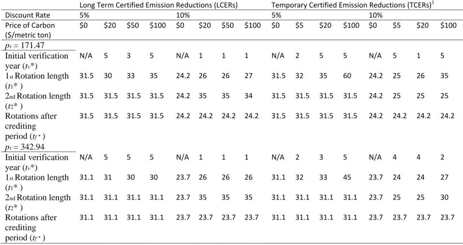
Tables 3 and 4 summarize optimal rotation intervals and initial verification period choice under lCERs for Philippine Mahogany and Tanazanian Neem, respectively.5 Simulated values for tCERs from Galinato and Uchida (forthcoming) are also presented for comparison. The Faustmann rotation age is 31.5 years for Mahogany and 9.8 years for Neem when the discount rate is 5%. At higher values of carbon prices, lower timber prices and lower discount rates, the optimal rotation interval is longer. Similar to the case where tCERs are generated, rotation intervals during the project are not necessarily the same.
There is only one rotation fully incorporated in the 60 year crediting period for Mahogany at a 10% discount rate. This is in contrast to the tCERs case where there are two full rotations within 60 years under the same conditions. When the lCERs policy is established, landowners have an incentive to lengthen rotation intervals to avoid incurring a harvesting
5
penalty. In order to fully avoid the penalty, the landowner can wait until the end of the project after 60 years as shown in the case where the discount rate is 10%.
For Tanzania, there may be 4 to 7 complete rotations within the 60-year project depending on the price parameters and discount rates. The most significant difference between tCERs and lCERs occurs especially when carbon prices reach $100 per ton of carbon. Under tCERs, the price increases rotation intervals up to 10 years but this is not the case with lCERs. The effect of a harvesting penalty may again explain why this occurs. Delaying harvest reduces the present value of the penalty, all things equal. However, it may also increase the nominal value of the penalty because it increases the distance between the volume before and after harvest. Thus, landowners may not increase rotations intervals too much in the presence of a harvesting penalty.
It appears under the lCERs program that the initial verification period is chosen so that the harvest date during the first rotation interval coincides with the last verification period. The initial verification period starts as early as year 1 of the first rotation or as long as year 5. The initial verification choice, however, does not guarantee that the last verification period during each subsequent rotation interval corresponds to the harvest date. This result is similar to the tCERs program.
In general, an increase in carbon price does increase the optimal rotation interval under lCERs, however, the effect is not as dramatic as under tCERs. Given a discount rate of 5% and a timber price of $171.47 per cubic meter, rotation intervals increase from 35 to 60 years under tCERs when going from $20/tC to $100/tC. Given the same parameters, the rotation interval increases from 30 to 35 years under lCERs. This is likely due to the way in which certified emission reductions are counted. Recall that tCERs are based on total volume during the
verification while lCERs are based on marginal volume from the previous verification period. Under tCERs, there is a greater incentive to increase rotation intervals longer because marginal carbon revenue during each verification period increases as long as the tree continues to grow. However, under lCERs, there is less incentive to keep the rotation longer because marginal carbon revenues decrease because the growth of trees increase at a decreasing rate.
Some rotation intervals with lCERs may be shorter than the case with no carbon revenues. For example, in Philippine mahogany when the carbon price is $50 and $100 with the timber price of $342.94 per cubic meter, the rotation interval with lCERs is 30 years while the optimal rotation interval is 31.1 years without carbon revenues. The theoretical model suggest that the nominal value of the penalty can be reduced by decreasing the rotation length since doing so decreases the gap between volume of trees across rotations before and after harvest. The present value of the penalty can also be reduced by lengthening the rotation interval. In this case, the former effect outweighs the latter effect, and could therefore induce the landowner to harvest earlier than the Faustmann rotation.
4.4 Supply of carbon sequestration from lCERs
The average annual supply of carbon sequestered from lCERs is a function of the price of carbon and other parameters of the model. The supply of lCERs is affected by the rotation length during the 60-year crediting period as well as the initial verification choice.
Figure 3 illustrates simulated carbon supply curves for Philippines and Tanzania. Carbon supply curves of the two different tree species vary substantially in timber prices and discount rates across. In some cases, there is an initial positive sequestration response to higher carbon prices, followed by no response thereafter. For example, for Tanzanian Neem, carbon sequestration credits increase with carbon price up to about $20/tC, but then remain
approximately unchanged. In other cases (one case for Tanzania and two cases for the Phillipines), carbon sequestration is perfectly inelastic with respect to carbon price, and there is effectively little or no response especially as trees approach the maximum volume function.
Finally, there are cases in which the carbon supply curve bends backwards and then increase again, such as Tanzanian Neem at a timber price of $106.67 and r=0.1 in Figure 3. This particular shape of the supply curve from lCERs can be attributed to the penalty imposed in the first verification after harvest. Recall that there are opposing incentives for the landowner to shorten or lengthen the rotation interval to avoid or reduce the penalty. When carbon prices are relatively low, marginal increases in the carbon price can increase rotation length leading to more carbon credits. However, over a higher range of carbon prices, the incentive to avoid the penalty is significant. Because the penalty is based on the difference in volume of trees before and after harvest, the landowner has an incentive to reduce the penalty by shortening the rotation interval thereby reducing this difference. Alternatively, the penalty can be pushed back to a later date reducing the present value of the penalty. Over a carbon price range of $50/tC to $100/tC when the interest rate is 10% for the Philippines, carbon supply decreases; rotation intervals are shorter because the former effect dominates the latter effect. Once the carbon price goes beyond $100/tC for Philippine Mahogany, carbon revenues become very significant and the latter effect now dominates the former effect.
It is clear from Figure 3 that there are limits to the incentive and ability to increase carbon biomass on a given plot of land. For Tanzanian Neem, annual accredited carbon dioxide sequestration does not go above about 0.95 metric tons per hectare per year for the lower timber price ($106.67) and does not go above about 0.60 metric tons per hectare per year for the lower timber price ($213.34) and higher discount rate. The former limit corresponds to a longer
rotation length, and the latter corresponds to a shorter rotation length. It is important to remember that even though there are limits to carbon sequestration supply response at the intensive margin the lCERs mechanism provides an incentive to move more land into forestry, thereby likely increasing carbon sequestration. In the case of Neem at a timber price of $213.34 and an interest rate of 10%, returns to carbon have little effect on carbon supply at all. This is mainly because carbon revenues, in this case, are a small proportion in total earnings for the landowner, and therefore has little effect on rotation choice when timber prices are high.
LCER-based carbon supply curves differ significantly from tCER-based carbon supply curves. Galinato and Uchida (forthcoming) obtain strictly increasing carbon supply curves asymptotic to the maximum production capacity of the tree without any backward bending areas. The main difference between the two policies that significantly affects the shape of the supply curves is the presence and design of the penalty.
We find that the price of timber and the discount rate significantly affects the degree to which the supply curve bends backwards. When the price of timber is relatively low and the discount rate is relatively high, the range in which the supply curve bends backward is larger for both tree species. This is consistent with our explanation based on the design of the penalty because relatively lower timber prices imply that the share of carbon revenues in the total net earnings of the landowner is larger. Also, the higher discount rate implies that the future value of a penalty is substantially lower when harvesting is pushed to a later date. The landowner will be more sensitive to changes in carbon prices given these two cases.
5. Conclusion
Implementing long term certified emission reductions under the Clean Development Mechanism has some interesting and, for practical policy implementation, problematic effects on
optimal rotation intervals and carbon credit generation of afforestation or reforestation programs. Adopting lCERs could result in heterogeneous rotation intervals because verification periods are administered in five-year intervals. The structure of the penalty during harvest could induce longer or shorter rotation intervals than the case without any harvesting penalties. Theoretically, the landowner can decrease the present value of the penalty by delaying harvest later for a constant penalty amount. However, the nominal value of the penalty is increasing in rotation interval length because it is based on the difference in volume before harvest and after harvest. Because of this interplay between the timing of penalties vis-à-vis harvest, practical efforts to predict or induce specific forest owner sequestration behavior at the intensive margin are likely to be imprecise.
In our simulations, we find several idiosyncratic characteristics of carbon supply at the intensive margin. In some parameterizations of timber price and interest rates, there is a backward bending region of the supply curve, which tends to be more pronounced when timber prices are relatively low and discount rates are high. In general, different parameterizations lead to substantially different asymptotes of carbon supply in response to carbon price. In some instances, there is little carbon supply response at the intensive margin.
Despite the complications and weaknesses of tCERs and lCERs, they do predictably increase soil expectation values from forestry. To the extent that standing forests are an effective medium for sequestering carbon relative to other land uses, remuneration for carbon sequestration via these instruments will tend to result in land conversion toward forestry.
One interesting question from a welfare standpoint is to derive how far the lCERs mechanism is from maximum social welfare and compare these results with tCERs. Given the inefficiencies of implementing tCERs, Galinato and Uchida (2010) measured the amount of
social welfare lost compared to a socially optimal policy and found only a 2% loss in social welfare with the tCERs policy at most. It would be useful to measure such welfare losses for lCERs. Another interesting question for future research is a comparison of the adoption of such a policy between risk-averse landowners. From our analysis, risk-neutral agents who maximize profit likely compare surplus between tCERs and lCERs in deciding what instrument to generate. In this case, one would derive higher returns from lCERs, all else equal. However, given potential uncertainty in the growth of trees and carbon uptake potential of different species, it would be interesting to see how risk-averse agents would view the two programs.
References
Binkley, C.S. and G.C. Van Kooten (1994), ‘Integrating climatic change and forests: economic and ecological assessments’, Climatic Change28: 91-110.
Bird, D.N., M. Dutschke, L. Pedroni, B. Schlamadinger, and A. Vallejo (2004), ‘Should one trade tCERs or lCERs?’, Policy Brief from the Environment and Community based framework for designing afforestation, reforestation and revegetation projects in the CDM: methodology development and case studies (ENCOFOR),
Available at: http://www.joanneum.at/encofor/publication/policy_briefs.html.
Cacho, O.J., R. L. Hean and R.M. Wise. 2003. “Carbon-accounting methods and reforestation incentives.” Australian Journal of Agricultural and Resource Economics. 47(2): 153-179.
Carbonpositive. 2009. “CDM forest projects approved for Uganda, Paraguay.” Carbon news and info. Available at: http://www.carbonpositive.net/viewarticle.aspx?articleID=1683.
CDM Rulebook, 2009a. A-Z Items, Temporary certified emission reduction (tCER),
http://cdmrulebook.org/380, last retrieved on 12/14/2009.
CDM Rulebook, 2009b. A-Z Items,Long-term certified emission reduction (lCER)
http://cdmrulebook.org/332, last retrieved on 12/14/2009.
Covar, R. (1998), ‘Carbon Sequestration Function of the Makiling Forest Reserve’, Thesis, UP at Los Banos Laguna, Philippines.
Dutschke, M, B. Schlamadinger, J.L.P. Wong, and M. Rumberg (2005), ‘Value and risks of expiring carbon credits from afforestation and reforestation projects under the CDM’, Climate Policy5: 19-36.
ECX. 2009. European Climate Exchange monthly data for October 2009. Available at: http://www.ecx.eu/ECX-Monthly-Report.
Galinato, G.I. and S. Uchida (forthcoming), ‘The Effect of Temporary Certified Emission Reductions on Forest Rotations and Carbon Supply’, Canadian Journal of Agricultural Economics.
Galinato, G.I. and S. Uchida (2010), ‘Evaluating Temporary Certified Emission Reductions in Reforestation and Afforestation Programs’, Environment and Resource Economics. 46(1): 111-133.
Germain, M, A. Magnus, and V. van Steenberghe (2007), ‘How to design and use the clean development mechanism under the Kyoto Protocol? A developing country perspective’, Environment and Resource Economics38: 13-30.
Guthrie, G. and D. Kumareswaran, Dinesh. 2009. “Carbon Subsidies, Taxes and Optimal Forest Management.” Environmental and Resource Economics, v. 43, iss. 2, pp. 275-93
Hoen HF, Solberg B (1997) CO2 – Taxing, timber rotations and market implications. Critical Review in Environ Science and Technology 27:S151-162
Lee, H-C, B. McCarl and D. Gillig. 2005. The Dynamic Competitiveness of US Agricultural and Forest Carbon Sequestration. Canadian Journal of Agricultural Economics. 53(4): 343-357.
Nordhaus WD (1991) The cost of slowing climate change: A Survey. Energy Journal 12(1):37-66
Olschewski, R., P.C. Benitez, G.H.J. de Koning and T. Schlichter (2005), ‘How Attractive are Forest Carbon Sinks? Economic Insights into Supply and Demand for Certified Emission Reductions’, Journal of Forest Economics 11(2): 77-94.
Plantinga, A.J. and R.A. Birdsey (1994), ‘Optimal forest stand management when benefits are derived from carbon’, Natural Resource Model8: 373-387.
Revilla, A.V. Jr., M.L. Bonita, and L.S. Dimapilis (1976), ‘Tree volume functions for Swietenia Macrophylla King, the Pterocarpus’, Philippine Science Journal of Forestry2: 1-7.
Richards KR (1992) Policy and research implications of recent carbon-sequestering analysis. In: Economics Issues in Global Climatic Change. Reilly JM, Anderson M (ed) Boulder Westview Press
Sedjo RA (1999) Potential for carbon forest plantations in marginal timber forests: The case of Patagonia, Argentina. RFF Discussion Paper 99-27
Sedjo, R.A. and A.M. Solomon (1989), ‘Climate and forests, greenhouse warming: abatement and adaptation’, in N.J. Rosenberg, W.E. Easterling III, P.R. Crosson, and J. Darmstadtered (eds), Resources for the Future, Washington DC, pp. 105-117.
Springer, D., J. Kennedy and R. MacNally. 2005. “Optimal Management of a Flammable Forest Providing Timber and Carbon Sequestration Benefits: An Australian Case Study.” The Australian Journal of Agricultural and Resource Economics . 49: 303-320.
Tewari, V.P. and V.S.K. Kumar (2002), ‘Development of top height model and site index curves for Azadirachta indica A. juss’, Forest Ecology and Management165: 67-73.
Tol, R.S.J. 2005. The marginal damage costs of carbon dioxide emissions: An assessment of the uncertainties. Energy Policy 33: 2064–2074.
UNFCCC. 2003. Modalities and Procedures for Afforestation and Reforestation Project
Activities under the Clean Development Mechanism in the First Commitment Period of the Kyoto Protocol. Decision-/CP.9. http://unfccc.int/cop9/latest/sbsta_l27.pdf (accessed February 1, 2010).
UNFCCC. 2006. Clarifications Regarding Methodologies for Afforestation and Reforestation CDM Project Activities. Annex 15 UNFCCC Project Design Document.
http://cdm.unfccc.int/Issuance/EB/022/eb22_repan15.pdf (accessed February 1, 2010).
UNFCCC. 2010. Registered Afforestation and Reforestation Projects Under CDM. http://cdm.unfccc.int/Projects/projsearch.html (accessed June 1, 2010).
Van Kooten, G.C., C.S. Binkley, and G. Delcourt (1995), ‘Effects of carbon taxes and subsidies on optimal forest rotation age and supply of carbon services’, American Journal of
Agricultural Economics77: 365-374.
Winjum, J.K., R.K. Dixon, and P.E. Schroeder (1992), ‘Estimating the global potential of forest and agroforest management practices to sequester carbon’, Water, Air, and Soil Pollution
Tables
Table 1 Parameters of the model
Parameter definition Mahogany in the
Philippines Neem in Tanzania Timber price (pv) per cubic meter
171.47 106.67 Harvesting cost (h) per cubic meter
35.23 21.33
Fixed cost of harvesting (Q) per hectare
803.97 156.89
Site index (I)
25 N/A
Wood density (WD) tons per cubic meter 0.56 0.52 Conversion factor to compute whole-stand
biomass from stem wood biomass (Cs) 1.6 1.2
Conversion factor to estimate the carbon content
of whole stand biomass (Cw) 0.5 0.5
Table 2 Per Hectare Soil Expectation Value of Carbon Forest Plantations with lCERs in the Philippines and Tanzania in an Infinite Rotation Planning Horizon (2001 US$)
Discount Rate 5% 10% Price of Carbon $0 $20 $50 $100 $0 $20 $50 $100 Philippines Net Benefits from Timber $5417.01 $5409.15 $5385.87 $5299.26 $435.82 $449.17 $449.17 $429.64 Net Benefits from Carbon including penalty $0 $296.95 $767.03 $1649.79 $0 $97.44 $240.91 $475.19 Soil Expectation Value (SEV) $5417.01 $5706.1 $6152.90 $6949.05 $435.82 $546.61 $690.08 $904.83 Tanzania Net Benefits from Timber $5243.09 $5254.54 $5254.54 $5237.98 $1964.42 $1962.83 $1959.65 $1940.59 Net Benefits from Carbon including penalty $0 $138.80 $347.01 $712.49 $0 $73.66 $188.50 $409.95 Soil Expectation Value (SEV) $5243.09 $5393.34 $5601.55 $5950.47 $1964.42 $2036.49 $2148.15 $2350.54
Table 3 Optimal Rotation and Initial Verification Periods in the Philippines in an Infinite Rotation Planning Horizon Under LCERS and TCERs
Long Term Certified Emission Reductions (LCERs) Temporary Certified Emission Reductions (TCERs)1
Discount Rate 5% 10% 5% 10% Price of Carbon ($/metric ton) $0 $20 $50 $100 $0 $20 $50 $100 $0 $5 $20 $100 $0 $5 $20 $100 pv = 171.47 Initial verification year (tv*)
N/A 5 3 5 N/A 1 1 1 N/A 2 5 5 N/A 5 1 5
1st Rotation length (t1* ) 31.5 30 33 35 24.2 26 26 27 31.5 32 35 60 24.2 25 26 35 2nd Rotation length (t2* ) 31.5 31.5 31.5 31.5 24.2 35 35 34 31.5 31.5 31.5 31.5 24.2 25 25 25 Rotations after crediting period (tf*) 31.5 31.5 31.5 31.5 24.2 24.2 24.2 24.2 31.5 31.5 31.5 31.5 24.2 24.2 24.2 24.2 pv = 342.94 Initial verification year (tv*)
N/A 5 5 5 N/A 1 1 1 N/A 2 3 5 N/A 4 4 2
1st Rotation length (t1* ) 31.1 31 30 30 23.7 26 26 26 31.1 32 33 45 23.7 24 24 27 2nd Rotation length (t2* ) 31.1 31.1 31.1 31.1 23.7 35 35 35 31.1 31.1 31.1 31.1 23.7 25 25 30 Rotations after crediting period (tf*) 31.1 31.1 31.1 31.1 23.7 23.7 23.7 23.7 31.1 31.1 31.1 31.1 23.7 23.7 23.7 23.7
Note: N/A means not applicable. 1
Table 4 Optimal Rotation and Initial Verification Periods in the Tanzania in an Infinite Rotation Planning Horizon Under LCERS and TCERs
Long Term Certified Emission Reductions (LCERs) Temporary Certified Emission Reductions (TCERs)1
Discount Rate 5% 10% 5% 10%
Price of Carbon ($/metric
ton)
$0 $20 $50 $100 $0 $20 $50 $100 $0 $5 $20 $100 $0 $5 $20 $100
pv = 106.67
Initial verification year (tv*)
N/A 5 5 1 N/A 3 3 4 N/A 5 5 5 N/A 3 3 5
1st Rotation length (t1* ) 9.8 10 10 11 7.9 8 8 9 9.8 10 10 15 7.9 8 8 10 2nd Rotation length (t2* ) 9.8 10 10 10 7.9 8 7 7 9.8 10 10 15 7.9 8 10 10 3rd Rotation length (t3* ) 9.8 10 10 10 7.9 8 8 9 9.8 10 10 15 7.9 8 10 10 4th Rotation length (t4* ) 9.8 10 10 10 7.9 9 7 9 9.8 10 10 15 7.9 9 10 10 5th Rotation length (t5* ) 9.8 10 10 10 7.9 8 8 7 9.8 10 10 7.9 8 10 10 6th Rotation length (t6* ) 9.8 (11) (11) (10) 7.9 8 7 9 9.8 10 10 7.9 8 10 10 7th Rotation length (t7* ) 7.9 9 8 9 7.9 9
Rotations after crediting period (tf*)
9.8 9.8 9.8 9.8 7.9 7.9 7.9 7.9 9.8 9.8 9.8 9.8 7.9 7.9 7.9 7.9
pv = 213.34
Initial verification year (tv*)
N/A 5 5 5 N/A 3 3 3 N/A 5 5 5 N/A 3 3 4
1st Rotation length (t1* ) 9.5 10 10 10 7.5 8 8 8 9.5 10 10 10 7.5 8 8 9 2nd Rotation length (t2* ) 9.5 10 10 10 7.5 7 7 7 9.5 10 10 10 7.5 7 7 10 3rd Rotation length (t3* ) 9.5 10 10 10 7.5 8 8 8 9.5 10 10 10 7.5 8 8 10 4th Rotation length (t4* ) 9.5 10 10 10 7.5 7 7 7 9.5 10 10 10 7.5 7 7 10 5th Rotation length (t5* ) 9.5 10 10 10 7.5 8 8 8 9.5 10 10 10 7.5 8 8 10 6th Rotation length (t6* ) 9.5 (11) (11) (11) 7.5 7 7 7 9.5 10 10 10 7.5 7 7 10 7th Rotation length (t7* ) 7.5 8 8 8 7.5 8 8
Rotations after crediting period (tf*)
9.5 9.5 9.5 9.5 7.5 7.5 7.5 7.5 9.5 9.5 9.5 9.5 7.5 7.5 7.5 7.5
Note: N/A means not applicable. 1
Figures
Source: Based on Figures 2 and 3 of Bird et al. (2004).
Figure 1 The lCERs mechanism
Figure 2 The tCERs mechanism
2012 2017 2022 2027 2030 2010 tCERs2012 tCERs2022 tCERs2017 tCERs2027 GHG accredited Cumulative GHG in sink Timber Harvesting in 2020
Source: Bird, et al. 2004 2012
2010 2017 2022 2027 2032 2010 2012
Carbon supply curves for Tanzania
0 50 100 150 200 250 0.5 0.6 0.7 0.8 0.9 1
Annual Accredited Carbon Dioxide (metric tons/Ha/Yr)
Ca rb on Pr ic e( $/ to n) ptim=106.67 r=0.05 ptim=106.67 r=0.1 ptim=213.34 r=0.05 ptim=213.34 r=0.1
Carbon supply curves for the Philippines
0 50 100 150 200 250 1 1.5 2 2.5
Annual Accredited Carbon Dioxide (metric tons/Ha/Yr)
Ca rb o n Pr ic e ($ /t on) ptim=171.47 r=0.05 ptim=171.47 r=0.1 ptim=342.94 r=0.05 ptim=342.94 r=0.1
Note: The variable ptim stands for timber price, and r is the interest rate.