Title:
Analysis of microtomographic images in automatic defect localization
and detection
Author:
Mariusz Marzec, Piotr Duda, Zygmunt Wróbel
Citation style:
Marzec Mariusz, Duda Piotr, Wróbel Zygmunt. (2020).
Analysis of microtomographic images in automatic defect localization and
detection. "Machine Vision & Applications: an international journal" (Vol. 31,
https://doi.org/10.1007/s00138-020-01084-3
O R I G I N A L P A P E R
Analysis of microtomographic images in automatic defect localization
and detection
Mariusz Marzec1 ·Piotr Duda1·Zygmunt Wróbel1 Received: 19 August 2019 / Revised: 7 March 2020 / Accepted: 20 April 2020 © The Author(s) 2020
Abstract
The paper presents a fast method of fully automatic localization and classification of defects in aluminium castings based on computed microtomography images. In the light of current research and based on available publications, where such analysis is made on the basis of images obtained from standard radiography (x-ray), this is a new approach which uses microtomographic images (μ-CT). In addition, the above-mentioned solutions most often analyze a pre-separated portion of an image, which requires the initial operator interference. The authors’ own pre-processing methods, which allow to separate the element area and potential defect areas fromμ-CT images, and methods of extraction of selected features describing these areas have been proposed in the solution discussed here. A neural network trained using the Levenberg–Marquardt method with error backpropagation has been used as a classifier. The optimal network structure 20–4–1 and a set of 20 features describing the analysed areas have been determined as a result of performed tests. The applied solutions have provided 89% correct detection for any defect size and 96.73% for large defects, which is comparable to the results obtained from methods using x-ray images. This has confirmed that it is possible to useμ-CT images in automatic defect localization in 3D. Thanks to this method, quantitative analysis of aluminium castings can be carried out without user interaction and fully automated. Keywords Image analysis·Image processing·Neural networks·Segmentation·μ-CT microtomography·X-CT computed tomography·X-ray
1 Introduction
Tomographic images are good material for research in the field of image analysis. They are used in many fields of sci-ence and technology. In medical applications, tomographic images are used in the diagnosis and assessment of various diseases, such as concussion [1], visualization of internal organs [2], or bone imaging and examination [3]. Tomogra-phy is often used in museology to preserve works of art. It is very important in the preservation of wooden works of art [4]. In forensic science, tomography supports forensic-medical diagnostics, facilitating autopsy and making it more accurate [5]. Recently, computed tomography and microtomography have been extensively used in industry, to study production quality, in reverse engineering and technology [6–9].
Cur-B
Mariusz Marzec1 Department of Computer Biomedical Systems, Institute of Computer Science, University of Silesia, ul. Bedzinska 39, 41-200 Sosnowiec, Poland
rent examples of applications in medicine and industry have been discussed in [10]. The quality control process also uses other techniques of non-invasive assessment of aluminium castings: ultrasonic methods, eddy currents and pulsed ther-mography [11]. In the study presented in this paper, the authors focused on the analysis of tomographic images used in the quality control of aluminium castings. Standard quality assessment of this type of elements with the use of computed tomography is characterized by high labour intensity and the need for visual analysis of thousands of images (obtained as a result of reconstruction) for each element tested. There are problems related to the lack of repeatability in the visual analysis and relativity of the assessment process. It seems to be possible to improve and speed up such tasks by using computers. However, it requires specialized algorithms that will enable to perform these tasks automatically. The devel-opment of such algorithms may open up the potential for scalability of these solutions by using faster hardware or par-allel calculations (each image can be analysed by another core). The paper presents the study aimed at developing a comprehensive algorithm for locating potential defect areas
based on image processing methods, proposing a set of fea-tures describing the studied areas and building a classifier based on a neural network.
2 Related work
The issue of locating and assessing defects in aluminium castings is very important from the point of view of the qual-ity control process. Its reliabilqual-ity and effectiveness have a big impact on safety in the subsequent use of construction elements created in this process. Current solutions and soft-ware packages allow for manual selection of defect areas, a semi-automatic process of calculating parameters describ-ing the structure homogeneity. Dependdescrib-ing on the needs, image binarization is performed manually for an experi-mentally defined brightness threshold. Such solutions are offered by practically all software packages intended for image analysis. However, the area of analysis is important in this case, because it must be related to the interior of the object. The user most often locates defect areas by view-ing hundreds of images representview-ing layers of the examined element, and then, using the basic image processing meth-ods, performs quantitative analysis on the selected cutting planes of the object. An example of such a solution is the VGStudio package [12]—Fig.12d (left). The user’s task is to define operating parameters, e.g. binarization threshold and some additional information related to, for example, the number of pixels on the edge of the object that can be closed to mark the void as the internal porosity of the object. The application algorithm combines the porosities on individual layers and calculates their total volume and other features. In the end, a list of pores is obtained, along with the volume and location of the centre of gravity. Fur-ther analysis is carried out in accordance with the client’s guidelines. The problem is porosity at the walls of objects and open porosity created as a result of other technological processes. Other software packages used in the laboratory to determine porosity are ImageJ [13] and CTAN [14], which offer similar capabilities in porosity analysis for flat images. Taking into consideration the high time-consuming nature of the activities described above, the need for user con-trol and the potential for using computers in processing and analysis of such images, the authors have developed a com-prehensive defect localization algorithm based on computed microtomography (μ-CT) images. The authors have anal-ysed the available literature in terms of existing solutions and observed a large number of publications in this field, which proves the importance of the problem and the purposefulness of the research undertaken. Among the examples, there are attempts at locating defects and assessing them in a more or less automated way using specialized image analysis algo-rithms. The following are examples of solutions for visible
light, based on standard x-ray and computed tomography (x-CT). In publication [15], the authors presented a method for the assessment and classification of surface defects in aluminium castings in visible light. A set of features was proposed (area, Feret elongation, compactness, roughness, length, breadth), which described the studied areas. A neu-ral network was used as a classifier, and the studied set was divided into three subsets: 70%—training, 15%—validation, and 15%—test. The training process lasted until the network continued its improvement on the validation set. The test set yielded the following results: 90% for correct and 10% for incorrect detection. However, the authors do not men-tion the number of images in the studied set, which makes it difficult to objectively evaluate the results obtained. Impor-tantly, due to the analysis of only the surface of castings, this method does not allow for the assessment of very significant defects formed inside the object. Another example [16] is the method of defect localization in aluminium or magnesium castings. Images obtained from x-ray were initially subjected to normalization of size and scale and processed with a fil-ter with an experimentally selected mask. Then, affil-ter using edge detection, the algorithm determined potential areas for further analysis. The geometrical parameters of the areas were determined on an 8-bit grayscale image. The following characteristics describing the areas were selected: perimeter, surface area, Feret diameters, Feret coefficient, circularity coefficient and dimensionless shape coefficient, Malinowska coefficient and moments. The set was randomly divided into 3 subsets, i.e. training (50%), validation (25%) and test (25%), and normalized. Data prepared in this way were analysed for several selected models of neural networks, including a multilayer perceptron (with 9–71–1 structure), network of radial base functions, probabilistic neural network (with 9– 33–1 structure). The best results of detection efficiency were obtained for the PNN (0.909) and MLP (0.813) networks. However, the authors do not mention how many images and elements were analysed, hence it is difficult to assess the uni-versality and scope of applicability of the algorithm. In paper [17], the authors developed the method described in [16] by adding the possibility of classifying the types of determined defects in accordance with the ASTM E155 standard [18]. 300 images having a resolution of 1760×2140 pixels were used in the study. The localization process was similar to that described in [16]. The coefficients describing the detected, interesting areas, i.e. surface area, perimeter, Feret diame-ters, circularity and roundness coefficients, were adopted in the defect type classification process. A neural network was used as a block of classification. The selection of features fed to the network input was determined using a genetic algo-rithm. The best results were obtained for the network with the MLP 5-27-108 structure—the effectiveness of defect type classification was 0.93. Detection efficiency was as in [16]. Another solution was proposed in [19] where the algorithm
was designed to classify the designated area into two classes: defect (D) or technological area (regular structures-RS). 72 x-ray images with a resolution of 572×768 pixels were used in the study. 25% of the examined areas (defects) were the result of a technological process, the remaining 75% were artificially made by drilling holes with a small diameter. As a result, 424 potential areas with 214 defects and 210 artificial holes were obtained. It was assumed that defects could be characterized as groups of pixels in the image with a bright-ness level significantly different from their surroundings. The potential areas were located on the basis of pixel brightness analysis and edge detection. For this purpose, the LOG filter in combination with the zero crossing algorithm was used. The result was a binary image of the edges surrounding the potential defect areas. In the next step, a set of parameters describing the designated areas was determined. 8 parame-ters were adopted, including 3 geometrical ones and 5 related to area brightness (height, area width, surface area, mean brightness, mean second derivative values of pixels, crossing line profile, standard deviation of the vertical and horizontal profiles and high contrast ratio). The feature vector obtained in this way was fed to the input of the neural network. The experimentally selected network structure for which the best results were obtained contained one hidden layer with 11 neurons (8–11–1 network structure). The effectiveness of the algorithm was evaluated using cross-validation and the result was 90%. Unfortunately, the study did not take into account the situation when technological holes are much larger than defects and their shape is not similar to a circle. The authors in [20] proposed a defect detection method based on a sequence of x-ray images (AMVI—Automated Multiple View Inspec-tion) taken for the test element. In the first stage, the method involved taking a series of images and automatic marking of potential defects in all the images. In the second stage, tracking was performed for each selected area. As a result of the study, it was found that only the areas correspond-ing to the actual defects were tracked correctly in the entire sequence of images because the changes in their position were closely related to the change in the position of the exam-ined element. The detection efficiency of 85.71% (TP / D) was achieved—Table3. In papers [21–23], the authors dis-cussed the principle of x-CT (x-ray computed tomography) andμ-CT (microtomography) [23] as well as the process of image reconstruction and visualization. The advantages of x-CT-based methods in relation to standard radiography were also highlighted (the option of determining distribution, size and morphology of defects). The authors evaluated the defects using specially prepared software, but the process was carried out manually. Localization and measurement of defect parameters were performed by an operator. Due to the manual observation and measurement, the effectiveness of the developed solution was not presented. In publication [24], the authors discussed the current state of research related to
x-ray image analysis and processing in defect localization tasks and presented a brief review of defect recognition meth-ods used so far. Next, the defect recognition methmeth-ods chosen by the authors and their effectiveness for a sample set were presented. The set consisted of 47,500 fragments of x-ray images sized 32 ×32 pixels with or without defect areas. Some selected computer vision methods were used (deep learning, sparse representations, local descriptors and tex-ture featex-tures). The best recognition results equal to 97% were obtained for the LBP descriptor (Local Binary Pattern) and the SVM linear classifier. When analysing the available liter-ature, it can be observed that most solutions are based on the popular method of x-ray radiography. In these cases, images obtained as a result of x-raying the whole test element are analysed. There are also examples of using computed tomog-raphy, but the analysis process is performed manually. The main problems that appear in the above solutions are difficul-ties with the full automation of the image analysis process, the use of prepared image portions containing interesting areas, the need to adjust algorithm parameters or pre-select the areas. Taking into account the advantages of x-CT and
μ-CT methods described in [20,22,23] and potential possibil-ities, this paper proposes using these imaging methods in the process of automated defect localization and classification. This approach enables to detect defects, which are invisible when using standard techniques, and will provide the possi-bility of automatic estimation of the volume of such defects in the future.
In summary, the novelties of this method include:
– fully automatic segmentation of the tested elements in
μ-CT images;
– no need to adjust the algorithm parameters;
– a method of local threshold determination to eliminate groups of pixels on the edges of elements;
– a method of potential defect area detection using struc-tural elements with a variable mask size;
– a proposal of a set of decryptors to describe defect areas; – a proposal and construction of the D/ND area classifier
using a neural network.
Due to the large number of studied images obtained for each element, the use of computer techniques seems neces-sary and justified. When analysing the available literature, the authors failed to find examples of algorithms for fully automatic defect localization that use images obtained from computed tomography (x-CT and μ-CT). Therefore, the effectiveness of the proposed method has been compared with selected solutions based on images obtained from stan-dard radiography (x-ray).
3 Material: collection of images
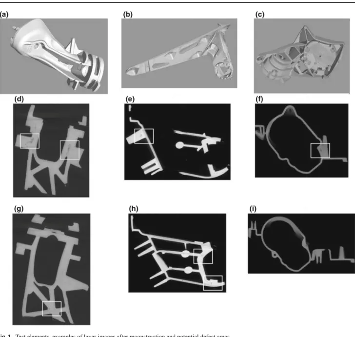
Three aluminium elements with different structure, wall thickness and size, previously subjected to standard, manual quality control, were used in the study. The images were taken using the GE Phoenix v|tome|x high-resolution x-ray sys-tem (microtomograph) at 200 kV and 300µA in the Faculty Computed Microtomography Laboratory of the University of Silesia. The exposure time was 500 ms. A series of 2000 images was taken for each element and then reconstruction was performed. As a result, images of layers were obtained, out of which the images containing the test element were selected. In total, there were 1200 (400 for each element) images of layers with different resolutions (972 × 1848, 1276×1589, 1922×1657) depending on the size of the ele-ment. Among potential areas for classification, the number of actual defects was 1255 and the number of technological holes (which are not defects) was 2083 based on the expert’s assessment, with a total number of 3338 areas. Examples of images of the test elements in the form of 3D visualization and reconstructed layers are presented in Fig.1a–c. Image areas where defects appear in the casting structure, which are significant from the point of view of assessing the element quality (large size, irregular structure, lower brightness than the surroundings), are marked in Fig.1d–h. In these areas, the proposed algorithm should localize the existing defects. In the case of Fig.1i, the defects in the structure of the entire element do not occur. The presented images show large vari-ability of parameters in terms of brightness, size, shape of elements, number and size of technological holes, shape of areas of potential defects and artefacts related to the image acquisition process. The large variety of images enabled to verify the universality of the developed solution and test it in the widest possible range.
4 Overview of the proposed approach
The developed algorithm has been fully implemented in MATLAB. In order to facilitate the work, collection and presentation of results, an application with a simple user interface has been prepared. The scheme of the algorithm is presented in Fig.2and individual blocks are discussed in the following sections. The prepared set of images was automat-ically analysed by the algorithm and the values of parameters describing the designated areas were automatically deter-mined. Then, the expert assessed each designated area, classifying it into two classes: D—defect, ND—nondefect. The data obtained in this way (1255—D and 2083—ND) were used to train the classifier and test the entire algorithm. The parameters controlling the algorithm and the method of their determination are presented in Table 1. The only parameter set manually is the minimum defect size—ATMin.
For the test images (at the stage of preliminary analysis on a scale of 1:4), it was ATMinSc =3 pixels. The minimum ATMinScvalue enables to eliminate too small areas, irrelevant from the point of view of assessing the element quality and not being defects. The other parameters are set automatically. The initial element binarization threshold determined by the Otsu method allows to roughly determine the binary mask of the element. The local brightness threshold TL(determined for each tested pixel of the element) enables to eliminate pixels (with a brightness greater than the global threshold
TOtsu) located on the inner and outer edges of the element. This operation makes it possible to significantly reduce the number of individual pixels and small areas in the viccinity of the inner and outer edges of the element—Fig.4e, f—Eq. (1).
4.1 Preliminary assumptions
Based on expert knowledge and literature [19,25] it was assumed that the areas interesting from the point of view of defect localization are characterized by the following fea-tures:
– brightness of defect pixels is smaller than surrounding brightness within the test element;
– brightness of defect pixels is greater than brightness of surrounding pixels outside the element;
– groups of darker pixels on the edges of the element are not defects;
– defect areas are characterized by heterogeneous texture; – defect areas are characterized by an irregular shape; – size, shape, orientation and location of defects are
unknown;
– sizes of areas important from the point of view of the quality control process are greater than ATMinSc(Table1) (3 pixels in the image in scale 1:4—at the stage of area localization);
– some areas may be remnants of technological holes (on subsequent layers) and are not defects (these cases were the most difficult to classify).
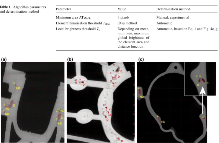
Figure3presents examples of potential areas selected by the algorithm and marked by the expert as D—defects and ND—nondefects. The area D in Fig.3a seem relatively easy to classify, their size is relatively large, the shape is irregular and their brightness is lower than the surrounding one. In turn, the areas assessed as ND are too small from the point of view of the quality control process. The situation looks slightly different in Fig.3b. The element is not as compact as in the previous case, hence small defects may also affect the quality of the element. Here, however, defects seem easy to classify taking into account geometrical parameters or brightness dis-tribution. Most of the pre-selected areas are characterized by much lower brightness in the defect area compared to the
Fig. 1 Test elements, examples of layer images after reconstruction and potential defect areas
surrounding background and irregular shape. The situation is a bit more difficult in the case of Fig.3c. Here, the areas of potential defects A, B are the result of a technological hole occurring in the previous layer. Such cases are the most diffi-cult to classify even in the case of manual evaluation. In these cases, the expert’s assessment was also based on the analysis of the previous and subsequent layers of the element. Based on the example of Fig.3, only areas marked by the expert as D should be classified positively by the algorithm as TP. The other areas are the result of technological holes in other layers and should be classified as TN. In the discussed algorithm, the preliminary assumptions described above were adopted so as to correctly locate and classify the cases described here.
4.2 Pre-processing and localization of areas
At this stage, the most important task for the algorithm was to separate the area of the examined element from the image background. The Otsu method [20,26] was used to determine the automatic binarization threshold of the image
TOTSU, which allowed to effectively separate the element from the background. The element is presented in Fig.4a and its binary mask in Fig.4b.
Due to high resolution, the images were scaled (in the ratio 1:4) at the stage of localization and detection of poten-tial areas, whereas at the stage of determining the values of area features the full-resolution images were used. The next pre-processing step was to determine groups of pix-els with brightness lower than the mean brightness TG in
Fig. 2 Block diagram of the developed algorithm
Table 1 Algorithm parameters
and determination method Parameter Value Determination method
Minimum area ATMinSc 3 pixels Manual, experimental Element binarisation thresholdTOtsu Otsu method Automatic
Local brightness thresholdTL Depending on mean, minimum, maximum global brightness of the element area and distance function
Automatic, based on Eq.1and Fig.4c, g
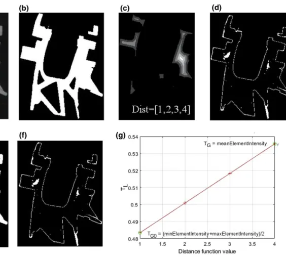
Fig. 4 Element and binary mask, distance function and resulting mask
the area of the test element and greater than the background brightness—TOtsu. A method was developed for automatic determination of the thresholdTGbased on the global mean brightness valueIMeanof the pixels belonging to the element (Fig.4a) and the local oneTL related to the distance of the examined pixel from the edge, determined by means of the distance function [27]. The values obtained from the distance function (Fig.4c)—calculated as the number of successive erosions with a ‘disk’ element SE sized 5×5 pixels) allowed for slight adjustment of the thresholdTL depending on the distance of the pixel from the edge of the test element.
The values obtained from the distance function (Fig.4c) enabled to slightly adjust the global threshold valueTGand determine the local thresholdTL(1)—Fig.4g. Figure4e (for comparison) shows groups of pixels determined based on the global thresholdTG, and Fig.4f—based onTL. It can be observed that as a result of this operation, the local threshold
TLhad a slightly lower value closer to the edge of the element,
which allowed to eliminate some dark pixels belonging to the edge of the element Fig.4f. On the other hand, inside the ele-ment, the value ofTLslightly increased (TL≤TG—Fig.4g), which allowed to locate slightly brighter pixels located near the searched areas. The threshold TL and darker pixels of element are determined based on Eq. (1):
TL(x,y)=TG0+TDist(x,y) ITL(x,y)= I(x,y) ifI(x,y)≤TL 0 ifI(x,y) >TL (1)
whereTLautomatically determined local threshold value for analysed pixel inx,y,TG0sum of min and max element inten-sity (pixels with inteninten-sity aboveTOtsu) divided by 2, TDist threshold increase based on value of distance function inx,
y—Fig.4c, g,I(x,y)analysed image—pixels with intensity aboveTOtsu,ITL(x,y)image with pixels with intensity≤TL.
Fig. 5 Elimination of edge pixels whose surroundings contain pixels with brightness below the designated threshold TOTSU(d–f)
Fig. 6 Preliminary analysis of
area masks by means of minimum filters of various sizes
In the next step, the edges of the element are removed by analyse the (3×3) surroundings of each pixel, based on (2):
IBin(x,y)= ⎧ ⎪ ⎨ ⎪ ⎩ 1 if min mi,niB3x3(x,y) (ITL(mi,ni)) >TOtsu 0 if min mi,niB3x3(x,y) (ITL(mi,ni))TOtsu IGB(x,y)=ITL(x,y)∗IBin(x,y) (2) whereITLimage with pixels with intensity≤TL,IBin(x,y) binary mask of pixels that satisfy the condition—(Fig.4d),
TOtsuautomatically determined threshold in image,IGB ele-ment in gray image after background elimination.
Pixels with brightness lower than the threshold TG and greater than the background brightnessTOTSUwere marked in the binary image representing the area masks. The pixels determined in this way belonged to 3 groups—Fig.4d, f:
– the remaining pixels belonging to the edge of the ele-ment whose lower brightness value is associated with the impact of background brightness;
– pixels belonging to the areas of technological holes or their remnants (in other layers)—not being defects; – proper pixels belonging to defect areas.
The last pre-processing operation was the elimination of large internal holes resulting from the shape of the element—Fig.6b. For this purpose, the flood-fill operation was used [27]. Then, based on the assessment of the shape of these areas, they were classified as large technological holes (areaValue/perimeterValue<1).
Large technological holes whose brightness was similar to the background brightness, i.e. lower thanTOTSU, were eliminated. Assuming an unknown size of defects, a solution based on the use of minimum filters with an increasing mask size was developed in order to locate groups of pixels within the element. The surroundings for each previously designated binary mask pixel (Fig.4d, f) were analysed with a 2 min-imum filters (erosion in gray image) to check if there were no background pixels. When a background pixel was present (the analysed pixel belonging to the edge or placed close to the edge), the determined minimum value in its surround-ings was smaller than the previously determined threshold
TOTSU. Such a pixel was then reduced and the area mask was reduced. This operation effectively eliminated edge pixels that were previously selected based on Eqs. (1), (2) and (3)
Is3x3(x,y)= min mi,niB3x3(x,y) (IGB(mi,ni)) Is5x5(x,y)= min mi,niB5x5(x,y) (IGB(mi,ni)) IBin3x3(x,y)= 1 ifIs3x3(x,y) >0 0 ifIs3x3(x,y)=0 IBin5x5(x,y)= 1 ifIs5x5(x,y) >0 0 ifI5x5(x,y)=0 (3)
where IGBintensity in image in grayscale Fig.6a, Eq. (1), Is3x3, Is5x5 image after using the minimum filter, IBin3x3, IBin5x5imagesIs3x3,Is5x5after thresholding Fig.6c, d.
An example of determining the minimum value of the sur-roundings is shown in Fig.5a (inside the element) and Fig.5d (on the element edge). It can be observed in Fig. 5b, c that the surroundings of the pixel are analysed in the increasing square area SE=3×3 and SE=5×5 but there are no dark pixels (with intensity = 0) of the background so the mask is not reduced. Figure5e shows that in the 3×3 surroundings there are no background pixels, but in the 5×5 surround-ings they appear, and this mask pixel Fig.5d will be therefore reduced.
It can be observed in Fig.6that the reduced binary mask from Fig.4d, f after using minimum filters of increasing size ((SE=3×3, SE=5×5, SE=7×7) Fig.6c–e) does not change in the areas designated inside the element (the surface area and shape are the same), while the areas belonging to the edge of the element are reduced due to the lower pixel brightness of the background surrounding the test element. The conducted tests have allowed to determine that the mask sizes SE=3×3 and SE=5×5 are sufficient for effec-tive separation of potential areas of defects. The last stage of locating potential areas of defects was the comparison of their geometrical parameters. These area masks which in the binary images (after applying the minimum filters SE=3
×3 and SE=5 ×5—Fig.6c, d) had the same values of the surface area and centroid coordinates were classified as a potential defect regions within the element and were sub-jected to further analysis—Fig.6f. At this stage, the expert classified the whole set of the designated areas, selecting the areas of defects D and technological holes ND. Figure 6f shows the final result of this operation in the form of groups of pixels located inside the test element. The pixels near the edges have been completely removed. This procedure is shown in Algorithm 1.
Algorithm 1Location of potential defect areas
Input:Image of the element extracted from the background -IG B
Output:The list of potential defects and their parametersdLi st- Fig.6f
1:IBi n3x3binary image after using min. filter se=3x3 onIG Band pixels
intensity>0
2:IBi n5x5binary image after using min. filter se=5x5 onIG Band pixels
intensity>0
3: Number of binary regions onIBi n3x3-N3x3and onIBi n5x5-N5x5 - Fig.6c, d
4: Compute regions parameters : area, centroid and other (Table2) for areas onIBi n3x3,IBi n5x5
5:fori3x3=1:N3x3do 6: fori5x5=1:N5x5do
7: search regionR3x3(i3x3)andR5x5(i5x5)with equal area and centroid
8: if regions are equal theR3x3(i3x3)add to the defects listdLi st
9: end for 10:end for
4.3 Generation and selection of values of area
features
The areas designated by the method shown in Fig.6 were subjected to quantitative analysis in order to determine the values of their features.
In order to prepare a set of features describing defect areas, the available literature on the previously used x-ray descrip-tors [15–17,19,20], universal image descriptors [28,29] and complex methods, e.g. CNN-based descriptors [30,31], LBP [32] and unsupervised learning [33], was analysed.
During tests and preparation of the set of images, the correct defect localization and classification by the expert were mostly affected by the contrast, brightness inside and outside the area, its irregular shape, and, to a lesser extent, by a specific texture pattern. Therefore, area descriptors and statistical texture descriptors, which are similar to those pro-posed in the analyzed literature for x-ray images, and some universal descriptors were selected—Table2. More complex methods of generating features can achieve similar or even higher efficiency. Features will be generated automatically but these methods will require a much larger training set of images [30] . The methods based on LBP [32] are very popular and effective, but their computational complexity is slightly higher. Therefore, when analysing multiple layers, the analysis time may be longer. The situation is similar in the case of unsupervised feature generation methods pro-posed in [33]. Here, the authors also point out the need for more computing power.
After having analysed the available literature [15–17,19,
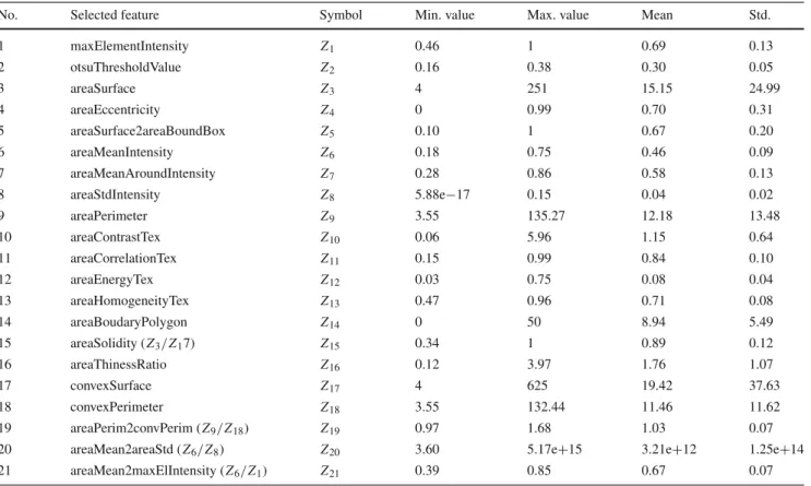
20,28,29], a set of 21 features was proposed by means of which the analysed areas were described. These features
formed a vector that was used in further research (4) dur-ing the construction of the classifier:
Z=(Z1,· · ·Z21)T (4) The set of features included basic geometrical, morpho-logical and texture parameters [28,29,34,35] and additional features determined on their basis. The selected parameters were described in sequence and presented in a graphical form in Fig.7. Table2presents the full list of the features used in further research together with basic statistical information before normalization. The parameter maxElementIntensity
is the maximum value of brightness in the image, and
otsuThresholdValueis the automatically determined thresh-old (Sect.4.2TOTSU). The parametersareaSurface, areaEc-centricity, areaSurface2areaBoundBox,areaMeanIntensity,
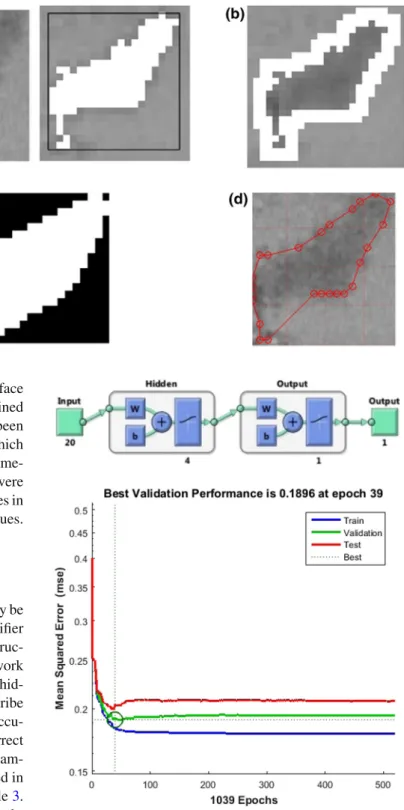
areaStdIntensitywere determined based on the binary mask of the designated area and the pixels of the examined image which the mask included Fig.7a. The parameter areaMea-nAroundIntensityis the mean brightness of the pixels around the studied area. The binary mask of the surroundings was generated as a result of dilation of the area mask with the element SE=3×3—Fig.7b.
The parameters areaContrastTex, areaCorrelationTex,
areaEnergyTex, areaHomogeneityTex are standard texture parameters generated on the basis of the normalized co-occurrence matrixNG[28,36] and described by the following equations (5) : ar eaContr ast T ex= i j (i− j)2Ng(i,j) ar eaCorr elati onT ex=
i j(i−μi)(j−μj)Ng(i,j) σiσj ar ea Ener gyT ex = i j Ng2(i,j) ar ea H omogenei t yT ex= i j Ng(i,j) 1+ |i− j| (5) wherei,jare the numbers of the row and column of the co-occurrence matrix NG,μi,μj andσi,σj are the means and standard deviations of the rowiand columnj.
TheareaBoudaryPolygonis the number of points around the boundary, which is a polygon—Fig.7d. The parameter
areaThinessRatiodescribed by Eq. (6) determines the irreg-ularity of the area shape.
Fig. 7 Graphic presentation of the selected parameters of the studied areas
TheconvexSurfaceandconvexPerimeter are the surface area and perimeter of the polygon surrounding the examined area—Fig.7c. The features Z15 and Z19−Z21 have been described in the form of dependencies, as a result of which they were determined in Table2. The determined parame-ters of features, before being fed to the classifier input, were normalized (relative to the minimum and maximum values in the range of 0–1) [37] to eliminate the impact of large values.
4.4 Classification of designated areas
After automatic localization of potential areas, which may be defects in the test element, a neural-network-based classifier was designed. After analysing the literature on the construc-tion of neural networks [25,37–39], a feedforward network with a sigmoid activation function with 9 inputs with 1 hid-den layer (4 neurons) and 1 output was proposed. To describe the quality of the tested classifier configurations, the Accu-racy (ACC) parameter (defining the best ratio of correct defect and nondefect detections to the number of all exam-ined areas) was used at this stage, which was also applied in compared publications [16,19,20] and described in Table3. At the beginning of the classifier construction process, a sub-set of 9 features was used, successively increased to 13, 18, 21 in order to compare the obtained results. The effects were unsatisfactory, ACC around 50%. Therefore, based on cor-relation, individual parameters were compared with the set values (areas of defects indicated by the expert) [37]. This demonstrated a particularly strong correlation of the vari-able Z7 (equal tor =0.44 with the set values) compared to other variables, which interfered with their impact on the obtained classification results. Therefore, the featureZ7was
Fig. 8 Structure of the neural network and number of epochs versus
mean square error
removed from the classifier input vectorZ, which positively influenced its operation, and a variant of the neural network with the 8–4–1 structure was adopted in further research. After removing the variableZ7, the features directly related to the brightness of areas and geometrical data (Z1−Z9)
Table 2 Statistical information on the area features
No. Selected feature Symbol Min. value Max. value Mean Std.
1 maxElementIntensity Z1 0.46 1 0.69 0.13 2 otsuThresholdValue Z2 0.16 0.38 0.30 0.05 3 areaSurface Z3 4 251 15.15 24.99 4 areaEccentricity Z4 0 0.99 0.70 0.31 5 areaSurface2areaBoundBox Z5 0.10 1 0.67 0.20 6 areaMeanIntensity Z6 0.18 0.75 0.46 0.09 7 areaMeanAroundIntensity Z7 0.28 0.86 0.58 0.13 8 areaStdIntensity Z8 5.88e−17 0.15 0.04 0.02 9 areaPerimeter Z9 3.55 135.27 12.18 13.48 10 areaContrastTex Z10 0.06 5.96 1.15 0.64 11 areaCorrelationTex Z11 0.15 0.99 0.84 0.10 12 areaEnergyTex Z12 0.03 0.75 0.08 0.04 13 areaHomogeneityTex Z13 0.47 0.96 0.71 0.08 14 areaBoudaryPolygon Z14 0 50 8.94 5.49 15 areaSolidity (Z3/Z17) Z15 0.34 1 0.89 0.12 16 areaThinessRatio Z16 0.12 3.97 1.76 1.07 17 convexSurface Z17 4 625 19.42 37.63 18 convexPerimeter Z18 3.55 132.44 11.46 11.62 19 areaPerim2convPerim (Z9/Z18) Z19 0.97 1.68 1.03 0.07
20 areaMean2areaStd (Z6/Z8) Z20 3.60 5.17e+15 3.21e+12 1.25e+14
21 areaMean2maxElIntensity (Z6/Z1) Z21 0.39 0.85 0.67 0.07
Table 3 Comparison of results obtained for the selected solutions
Method Number of images Total number of defects/nondefects ACCCVMean ACCCVMax Detection perfor-mance (DP) AUC Fig.9 D/ND TP+TND+ND TPD
Method 1 [16] N/A N/A N/A N/A N/A
81–90%
Method 2 [19] 72 214/210 90.3% N/A 0.96
95.3%
Method 3 [20] 72 238/253 N/A 85.71% N/A
Method 4 1200 1255/2083 86.5% 85.6% 0.89
Proposed method 89.1% 85.22%
were proposed as an input vector, which provided ACC= 81.81%. Then, attempts were made to verify the effective-ness by adding features related to the texture of the studied areas (Z10−Z13), which helped to obtain better results— ACC=85.23%. In the next stage, (Z14−Z18) parameters that define irregularities in the shape of the areas were added to the feature vector, yielding ACC=86.99%. Finally, the features artificially generated based on the basic features (Z19−Z21) were added, and the result obtained in this case was ACC= 89.01%. For each case, 5 network training/testing attempts were made and the best solution was chosen, which was a neural network with 20 inputs, 4 neurons in the hidden layer
and 1 neuron in the output layer (20–4–1)—Fig.8. A network output value greater than 0.5 was classified as a defect area. The system performance is analysed in terms of number of epochs versus MSE (Fig.8). The best validation performance in terms of MSE is 0.1896 at epoch 39.
4.5 Results and discussion
In order to fully evaluate the developed algorithm and the selected variant of the neural network and to compare it with the mentioned publications [16,19,20], three parameters were applied, i.e. Accuracy (ACC), Detection performance
Fig. 9 ROC curve for the best classifier variant (20–4–1)
(DP) and ROC curve (AUC—Area Under Curve), which are described in the form of equations in the respective columns in Table3. Figure9presents the ROC chart for the classifier in 20–4–1 configuration with the input vector of featuresZ
as below (7).
Z=(Z1, . . .Zn)T n∈ {1,2,3,4,5,6,8,9,
10,11,12,13,14,15,16,17,18,19,20,21}
(7)
The effectiveness of the developed algorithm was verified on the basis of error matrix analysis [19,37]. The values of TP, TN, FP, FN were determined from the error matrix and on their basis the basic measures of the classifier quality were
calculated. Situations in which the algorithm correctly identi-fied the actual areas of defects were adopted as TP (375). TN (638) were cases when the areas being technological holes or their remnants (on successive layers) were correctly rec-ognized as nondefects. FP detections (60) were situations when technological holes were recognized as defects, and FN (65) when defect areas were not identified. As a result, the following values were obtained: ACC = 89.01%, DP
=85.22% and AUC=0.89—Table3. The applied test set included 1138 randomly selected, potential areas for clas-sification, where the number of actual defects D was equal to 440 and ND =698. The authors could not find in the available literature algorithms intended for automatic local-ization and classification of defects for x-CT orμ-CT images after reconstruction. Therefore, Table3compares the effec-tiveness of the developed method with the selected solutions based on standard x-ray images, which were discussed above. The assessment was carried out on the basis of parameters proposed by other authors and the results obtained for test sets. The Accuracy parameter was presented as the best ACC value (ACCCVMax) and the mean value obtained from cross-validation ACCCVMean(when the authors presented such data in their publications).
In order to confirm the effectiveness of the classifier under different conditions (for different subsets of data), the model was evaluated (similarly as in [19]) by means of foldfold cross validation, for randomly generated 10 sets (training set to test set in a ratio of 9–1). The mean value in cross-validation was ACCCVMean =86.5% and DP= 85.6% (according to the formulas in Table3). The values were not much lower than the best results obtained at the stage of experiments with the classifier construction (where 2200 and 1138 areas were used as a training and test sets, respectively—described
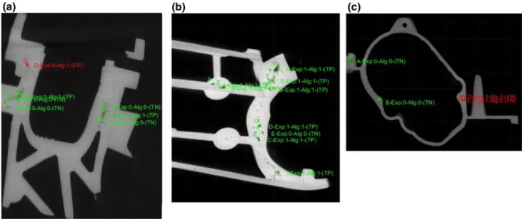
Fig. 11 Exemplary results: classification of
defects—green—consistent with the expert,
red—non-consistent with the expert (colour figure online)
above−4.4), which proves the correct and optimal choice of parameters. The average time of analysis of a single image with a graphical presentation of the results was less than 1 s. The calculations were performed on the computer with an Ryzen 5 processor working at 3.8 GHz.
Since the method [19] provided slightly better results, its implementation was prepared on the basis of [19,40] in order to verify its effectiveness and applicability in the examined
set ofμ-CT images. Then, tests were carried out using images from publication [19] and from theμ-CT image set prepared by the authors. Figure12a shows the results of the algorithm performance [19] in the x-Ray image from the set [19]— correctly detected defect area. Figure 12b, c are examples of how the algorithm from [19] works inμ-CT images. Fig-ure12b shows examples of defect area detection throughout the image and Fig. 12c—in the element sections. As can
Fig. 12 Examples of how the method [19] works for x-ray images from [19] (a) andμ-CT images (b,c). Manual measurement of the defect size in the myVGL applicationdleft and using the algorithmdright
be seen in the attached images, the high efficiency of the method used for x-Ray images [19] does not translate into its effectiveness inμ-CT images. The method does not correctly determine any of the defects, therefore its direct application inμ-CT is impossible. In these cases, the method proposed by the authors achieves incomparably better results, which confirms its effectiveness in the case ofμ-CT images.
When analysing the obtained results, it can be observed that similar effectiveness of the algorithm was obtained in relation to the compared publications (despite different image types), which confirms that it is possible to achieve
satisfac-tory results also for images obtained fromμ-CT. Analysis of this type of images additionally allows for localization of defects, which in standard methods may be invisible or hardly visible. Moreover inμ-CT, if the defect is not detected in one layer (due to the automatic selection of the algorithm param-eters), it is possible that it will be detected in the next layer, which globally increases the effectiveness of the entire solu-tion when combining informasolu-tion from all layers. Figure10
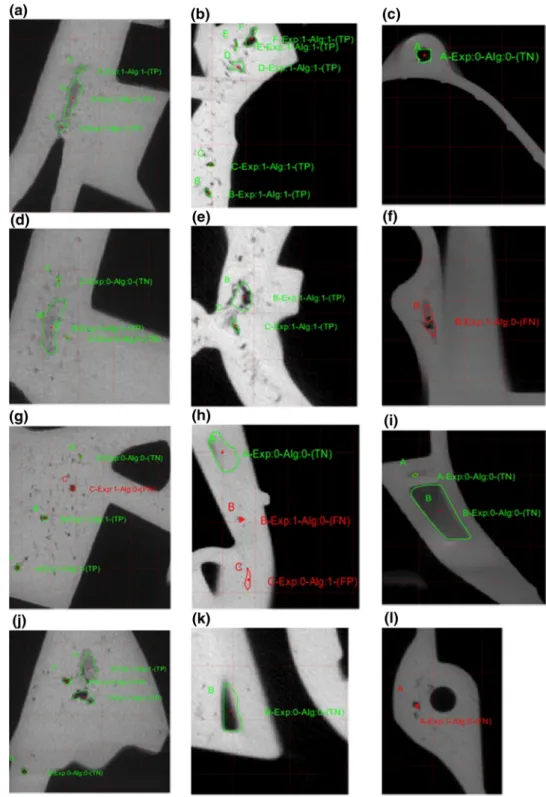
shows exemplary results of the developed algorithm for the images presented in Fig.3. Examples Fig.10a–c are defect areas indicated by the expert and by the developed algorithm.
Relevant cases consistent with the expert classification (TP, TN) are marked in green, erroneous cases (FP, FN)—in red. In addition, there is information about the expert and algorithm classification.
It can be observed that the algorithm correctly locates defects of relatively large sizes. It incorrectly marks the one area D, which the expert assessed as irrelevant from the point of view of the element quality—Fig. 10a. Further exam-ples are images in Fig.10b. Here, both the expert and the developed algorithm marked 9 areas as significant defects. The case in Fig.10c is quite interesting. The test element has a completely different structure from the previous ele-ments. Area A also appears here, which is the remnant of the technological hole in the previous layers but importantly, the algorithm reacts correctly and does not mark it as a defect. However, incorrect detection occurs in the case of areas C and D, marked by the expert but not by the algorithm (color red). These areas are relatively dark and have a small size, which may affect the classifier behaviour. To sum up, these examples show that in most cases the algorithm reacts cor-rectly only in the case of very small defects and its results are not always consistent with the expert’s assessment.
Further examples are shown in Fig.11, where the test areas are enlarged. As in Fig.10, each case is marked as TP, TN, FP, FN—classification consistent with the expert—green, non-consistent—red. It can be observed in Fig.11a, d, g, j how the algorithm easily locates almost all defect areas and cor-rectly classifies them. It detects both very dark areas Fig.11j and lighter ones Fig.11a, b. Unselected areas do not meet the size criterion, so they are not subjected to classification. In the case of Fig.11h area B, the algorithm incorrectly clas-sifies the area (FN). In the assessment of the casting quality, such a small area would not affect the test result. Similarly, in the case of Fig.11h area C, despite the FP classification, the size of the area is not significant. An interesting case of cor-rect classification of a technological hole (TN) is presented in Fig.11c, i, k. The algorithm, despite the large size of the areas, correctly classified them as Nondefects , which is con-sistent with the expert’s assessment (TN). Figure11f, l shows a defect classification error (B, A, respectively) despite the fairly good visibility of the defect during visual assessment— such cases indicate that the development and improvement of the algorithm may be the subject of further research.
Figure11l is a case when a technologcial hole, due to its shape and structure, is not selected at all for further classifica-tion. This confirms that the algorithm block eliminating clear technological holes also works correctly. The most important feature of a defect, from the point of view of casting qual-ity assessment, is its size. The examples in Figs.10and11
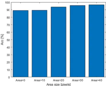
show that the proposed method locates and classifies larger, most significant defects with high efficiency. The results of the algorithm effectiveness obtained in the test set for defects of various sizes are presented in Table4and Fig.13.
Fig. 13 Detection efficiency depending on the defect area
Based on the results obtained and the examples presented, it can be concluded that the proposed algorithm is very effec-tive (Acc = 96.73%) in assessing larger, significant areas, and possible errors and lower effectiveness occur in the case of smaller, less significant defects.
In the process of generating features of areas, minimum surface area, perimeter and major axis length are determined for each defect. These values with known parameters of the microtomographic device allow for the quantitative assess-ment of the surface of each defect detected by the algorithm (in each tested layer) in mm2or mm. In the examined images, 1 image voxel corresponded to 75µm or 123µm (depend-ing on the image). Based on these values and Eq. (8), the real sizes of the defect areas can be determined.
AreaR=AreaPsc∗imgSc∗voxelRatio PerimR=PerimPsc∗imgSc∗voxelRatio DistR=DistPsc∗imgSc∗voxelRatio
(8)
where AreaR, PerimR, DistR real values in mm2 or mm, AreaPsc, PerimPsc, DistPscvalues in pixels (in scaled image), imgSc scale at which the image is processed, voxelRatio ratio of voxel size to 1 mm.
The results obtained can be used as input information for a decision system that will automatically assess the qual-ity of the tested casting. An example of a practical, potential application, where the discussed algorithm could completely automate the process of casting testing, is publication [41]. Its authors presented a method for assessing the quality of elements based on micro-tomographic images analysed semi-automatically by the operator and specialized software. Full automation of this process can significantly facilitate and accelerate the assessment of casting quality, as well as allow
Table 4 Detection efficiency depending on the defect area (89.01 % for all areas / 96.73 for the largest areas)
AreaPSc TP TN FP FN Def. count Non def. count Acc (%)
>0 375 638 60 65 440 698 89.01
>10 204 88 21 14 218 109 89.29
>20 107 58 7 4 111 65 93.75
>30 73 37 4 1 74 41 96.65
>40 61 28 2 1 62 30 96.73
for the analysis of large data sets in an unsupervised manner and presentation of the results in the form of reports with a quantitative assessment of the tested elements. An example comparing the results obtained during manual measurement and determined by the algorithm is presented in Fig.12d. The area perimeter and the largest area distance (determined manually and by using the proposed algorithm) reached the values from 17.72 to 19.44 mm and from 7.86 to 7.38 mm, respectively, which gives a relative measurement error 9.7% (area perimeter) and 6.5 % (area largest distance) compared to the manual measurement.
4.6 Conclusions
The paper proposes an original method of automatic local-ization and classification of defects inμ-CT images based on image analysis methods and neural networks. Compared to typical solutions based on x-ray images, an innovative approach has been proposed that enables to analyse tomo-graphic images of layers after reconstruction. Analysis of this type of images can allow for fully automatic acquisition of additional information (e.g. defect volume) or localiza-tion of defects hidden under the element fragments. At this stage of research, the proposed algorithm has obtained the effectiveness of correct detections similar to that of refer-ence methods based on x-ray images. The maximum value of ACC is 89% and the mean value obtained in cross-validation ACCCVMean=86.6% (Table 3). When the largest and most important defects were searched for, the algorithm efficiency reached even 96.73% (Table4).
The authors have also managed to optimize the network structure compared to the described solutions [16,19,20] (especially in the hidden layer), which has a positive effect on the classifier speed. The expert during the manual evalu-ation analysed the previous and next layers in addition to the test layer, so if the algorithm is further improved to work in a similar way, it will provide more information and will be more effective. This can be particularly important for areas which are the remnants of technological holes in the neigh-bouring layers and are not actual defects. Proposed method allows the fast and fully automated analysis single or set of
μ-CT images without user interaction and need for selection of image analysis parameters.
Open Access This article is licensed under a Creative Commons
Attribution 4.0 International License, which permits use, sharing, adap-tation, distribution and reproduction in any medium or format, as long as you give appropriate credit to the original author(s) and the source, provide a link to the Creative Commons licence, and indi-cate if changes were made. The images or other third party material in this article are included in the article’s Creative Commons licence, unless indicated otherwise in a credit line to the material. If material is not included in the article’s Creative Commons licence and your intended use is not permitted by statutory regulation or exceeds the permitted use, you will need to obtain permission directly from the copy-right holder. To view a copy of this licence, visithttp://creativecomm ons.org/licenses/by/4.0/.
References
1. Useche, J.N., Bermudez, S.: Conventional computed tomography and magnetic resonance in brain concussion. Neuroimaging Clin. N. Am.28(1), 15–29 (2018)
2. Okumura, M., Usumoto, Y., Tsuji, A., Kudo, K., Ikeda, N.: Analysis of postmortem changes in internal organs and gases using computed tomography data. Leg. Med.25(2017), 11–15 (2017)
3. Barak, M.M., Black, M.A.: A novel use of 3D printing model demonstrates the effects of deteriorated trabecular bone structure on bone stiffness and strength. J. Mech. Behav. Biomed. Mater. 78(2018), 455–464 (2018)
4. Okochi, T.: A nondestructive dendrochronological study on japanese wooden shinto art sculptures using micro-focus X-ray Computed Tomography (CT) Reviewing two methods for scanning objects of different sizes. Dendrochronologia38, 1–10 (2016) 5. Moskała, A., Wo´zniak, K., Kluza, P, Bolechała, F.,
Rzepecka-Wo´zniak,E., Kołodziej J, Latacz K.: Przydatno´s´c po´smiertnego badaniatomografii komputerowej z angiografi¸a (PMCTA) w s¸adowo-lekarskiejdiagnostyce przypadków ran kłutych i ciétych. ARCH. MED. S ¸AD.KRYMINOL., 2012, LXII, pp. 315–326 (2012)
6. Ratajczyk, E.: Rentgenowska tomografia komputerowa (CT) do zada´n przemysłowych. Pomiary automatyka Robotyka 5(2012), 104–113 (2012)
7. Królikowski, M., Burbelko, A., Kwa´sniewska-Królikowska, D.: Wykorzystanie tomografii komputerowej w defektoskopii odlewów z ˙Zeliwa sferoidalnego. Arch. Foundry Eng.14(4), 71–76 (2012)
8. Ewert U., Fuchs T.: Progress in digital industrial radiology Part II: computed tomography (CT). Badania Nieniszcz¸ace i Diagnostyka1-2 , 2017, pp. 7–14 (2017)
9. Le, V.-D., Saintier, N., Morel, F., Bellett, D., Osmond, P.: Investi-gation of the effect of porosity on the high cycle fatigue behaviour
of cast Al-Si alloy by X-ray micro-tomography. Int. J. Fatigue106, 24–37 (2018)
10. du Plessis, A., le Roux, S., Guelpa, A.: Comparison of medical and industrial X-ray computed tomography for non-destructive testing. Case Stud. Nondestruct. Test. Eval.6(Part A), 17–25 (2016) 11. Wilczek, A., Długosz, P., Hebda, M.: Porosity characterization of
aluminium castings by using particular non-destructive techniques. J. Nondestruct. Eval.34, 26 (2015)
12. https://www.volumegraphics.com/en/products/vgstudio-max. html
13. https://imagej.net/
14. http://bruker-microct.com/products/ctan.htm
15. ´Swiłło, S.J., Perzyk, M.: Surface casting defects inspection using video system and neural networks techniques. Arch Foundry Eng 13(4), 103–1069 (2013)
16. Dobrza´nski, L.A., Krupi´nski, M., Sokolowski, J.H.: Computer aided classification of flaws occurred during casting of aluminum. J. Mater. Process. Technol.167(2–3), 456–462 (2005)
17. Dobrza´nski, L.A., Krupi´nski, M., Sokolowski, J.H.: Methodology of automatic quality control of aluminum castings. J. Achiev. Mater. Manuf. Eng.20(1–2), 69–78 (2007)
18. https://www.astm.org/Standards/E155.htm
19. da Silva, R.R., Mery, D.: Accuracy estimation of detection of cast-ing defects in x-ray images uscast-ing some statistical techniques. In: PSIVT 2007: advances in image and video technology, pp. 639– 650 (2007)
20. Pizarro, L., Mery, D., Delpiano, R., Carrasco, M.: Robust auto-mated multiple view inspection. Pattern Anal. Appl.11(1), 21–32 (2008)
21. Arunmuthu, K., George Joseph, T., Saravanan: X-ray computed tomography based detection of casting defects in fatigue sam-ples. In: 25th National Seminar and International Exhibition, Non Destrucitve Evaluation, November 26–28 (2015)
22. Nicoletto, G., Anzelotti, G., Konecna, R.: X-ray computed tomog-raphy vs. metallogtomog-raphy for pore sizing and fatigue of cast Al-alloys. Procedia Eng.2(1), 547–554 (2010)
23. Nicoletto, G., Konecna, R., Fintova, S.: Characterization of microshrinkage casting defects of Al–Si alloys by X-ray computed tomography and metallography. Int. J. Fatigue41, 39–46 (2012) 24. Mery, D., Arteta, C.: Automatic defect recognition in X-ray
test-ing ustest-ing computer vision. In: 2017 IEEE Winter Conference on Application of Computer Vision (WACV), Santa Rosa, CA, USA (2017)
25. Osowski, S.: Sieci neuronowe do przetwarzania informacji (wyd.3), Oficyna Wydawnicza Politechniki Warszawskiej, p. 422 (2013)
26. Otsu, N.: A threshold selection method from gray-level histograms. IEEE Trans. Syst. Man Cybern.9(1), 62–66 (1976)
27. Tadeusiewicz, R., Korohoda, P.: Komputerowa analiza i przetwarzanie obrazów, Wydawnictwo Fundacji Post¸epu Teleko-munikacji, p. 280 (1997)
28. Marques, O.: Practical Image and Video Processing Using MAT-LAB, p. 704. Wiley, Hoboken (2011)
29. Gonzalez, R.C., Woods, R.E., Eddins Steven, L.: Digital Image Pro-cessing Using MATLAB 2e, p. 827. Gatesmark Publishing, London (2009)
30. Zhang, D., Han, J., Li, C., Wang, J., Li, X.: Detection of co-salient object by looking deep and wide. Int. J. Comput. Vis.120, 215–232 (2016)
31. Gao, Z., Zhang, H., Dong, S., Sun, S., Wang, X., Yang, G., Wu, W., Li, S.: Salient object detection in the distributed cloud-edge intelligent network. IEEE Netw.34, 216–224 (2020)
32. Xiao, B., Wang, K., Bi, X., Li, W., Han, J., Member, S.: 2D LBP an enhanced local binary features. IEEE Trans. Circuits Syst. Video Technol.29(9), 2796–2808 (2019)
33. Zheng, Y., Jeon, B., Sun, L., Zhang, J., Zhang, H.: Student’s t-Hidden Markow models for unsupervised learning using localised feature selection. IEEE Trans. Circuits Syst. Video Technol.28, 1 (2017)
34. Mery, D., Filbert, D.: Classification of potential defects in auto-mated inspection of aluminium castingusing statistical pattern recognition. In: 8th European Conference on Non-destructive Test-ing (ECNDT 2002), Barcelona, Spain (2002)
35. Sikora, R. , Baniukiewicz, P., Chady, T., Lopato, P., Psuj, G.: Artig-ical neural networks and fuzzy logic in nondestructive evaluation. In: 18th World Conference on Nondestructive Testing, Durban (2012)
36. Zieli´nski, K.W., Strzelecki, M.: Komputerowa analiza obrazu biomedycznego, PWN, Warszawa, p. 367 (2001)
37. Osowski, S.: Metody i narz¸edzia eksploracji danych. Wydawnictwo BTC, Legionowo, p. 388 (2013)
38. Tadeusiewicz, R.: Sieci neuronowe. Akademicka Oficyna Wydawnicza, Warszawa, p. 299 (1993)
39. Tadeusiewicz, R.: Odkrywanie wła´sciwo´sci sieci neuronowych przy u˙zyciu programów w j¸ezyku C#. Wydawnictwo Polskiej Akademii Umiej¸etno´sci, Kraków, p. 426 (2007)
40. Domingo, M.: Computer Vision for X-Ray Testing, Imaging, Sys-tems, Image Databases, and Algorithms, p. 347 (2015)
41. Le, V., Saintier, N., Morel, F., Bellett, D., Osmond, P.: Investigation of the effect of porosity on the high cycle fatigue behaviour of cast Al–Si alloy by X-ray micro-tomography. Int. J. Fatigue106, 24–37 (2017)
Publisher’s Note Springer Nature remains neutral with regard to
juris-dictional claims in published maps and institutional affiliations.
Mariusz Marzecis an assistant
pro-fessor in Department of Biomedi-cal Computer Systems at the Insti-tute of Computer Science, Sile-sian University in Katowice. His scientific interests are computer analysis and processing of images, biomedical images, databases and programming languages. He is an author and co-author of scientific publications in analysis and pro-cessing of biomedical images and developing database systems.
Piotr Duda is an assistant
pro-fessor in Department of Biomedi-cal Computer Systems at the Insti-tute of Computer Science, Sile-sian University in Katowice. His scientific interests are biomedi-cal engineering, tribology, micro-tomography and material engineer-ing. He is an author and co-author of scientific publications in the field of tribology and the use of microtomography in pharmacy and biomedical engineering.
Zygmunt Wróbelis the Director of Institute of Computer Science of Silesian University in Katowice. His scientific interests are com-puter analysis and processing of biomedical images and signals, and applications of information tech-nology in medicine and biotech-nology. He is an author and co-author of tens of scientific publi-cations in analysis and processing of biomedical images and infor-mation technology.
![Fig. 12 Examples of how the method [19] works for x-ray images from [19] (a) and μ-CT images (b, c)](https://thumb-us.123doks.com/thumbv2/123dok_us/1445539.2693488/16.892.80.815.76.785/fig-examples-method-works-ray-images-ct-images.webp)