Factor Utilisation and Productivity Estimates for the United Kingdom

Factor Utilisation and Productivity Estimates for the United Kingdom

Jens Larsen*, Katharine Neiss†

and Fergal Shortall‡

* Monetary Assessment and Strategy Division, Bank of England, Threadneedle Street, London EC2R 8AH, United Kingdom.

Tel: +44 207 601 3560. Email: [email protected].

† Monetary Assessment and Strategy Division, Bank of England, Threadneedle Street, London EC2R 8AH, United Kingdom.

Tel: +44 207 601 4588. Email: [email protected].

‡ Structural Economic Analysis Division, Bank of England, Threadneedle Street, London EC2R 8AH, United Kingdom.

Tel: +44 207 601 3094. Email: [email protected].

The views expressed in this paper are those of the authors and should not be interpreted as those of the Bank of England or the Monetary Policy Committee. We are grateful to John Muellbauer for providing us with data on the PUL. We thank two anonymous referees, Hasan Bakhshi, Charlie Bean, Ian Bond, Martin Eichenbaum, Phil Evans, Rain Newton-Smith, Steve Nickell, Evi Pappa, and Bank of England Seminar and Research Away Day participants for extremely useful comments and suggestions. We would also like to acknowledge prior work by Mark Astley that motivated this paper.

Copies of working papers may be obtained from Publications Group, Bank of England,

Threadneedle Street, London, EC2R 8AH; telephone 020 7601 4030, fax 020 7601 3298, e-mail [email protected].

Working papers are also available from the Bank’s Internet site at www.bankofengland.co.uk/wp/index.htm.

The Bank of England's working paper series is externally refereed.

Bank of England 2002 ISSN 1368-5562

Contents

Abstract 5

Summary 7

1 Introduction 9

2 A model of time-varying factor utilisation with labour adjustment costs 11

2.1 Households 11 2.2 Firms 14 2.3 Government 15 2.4 Market clearing 15 2.5 Equilibrium 15 2.6 Shocks 17

3 Calibration and impulse responses 17

3.1 Calibration 17

3.2 Impulse responses 19

4 Method 21

5 Estimated series for the United Kingdom 23

5.1 The capital-to-output ratio 23

5.2 Capital utilisation 24

5.3 Labour effort 26

5.4 Intensive margins 28

5.5 Total factor productivity 29

5.6 Aggregate factor utilisation 29

5.7 Accounting for changes in our derived series 32

6 Conclusion 34

Appendix 35

Data sources and description 36

Abstract

This paper derives series for capital utilisation, labour effort and total factor productivity from a general equilibrium model (based on Burnside and Eichenbaum, 1996) with variable factor utilisation and labour adjustment costs. Impulse responses from the model show that firms initially respond to unanticipated shocks by altering factor utilisation rates. In subsequent periods, firms adjust observable inputs such as physical capital and employment. As a result, utilisation rates are a leading indicator of firms’ hiring of both capital and labour.

We find that our estimate of capital utilisation tracks survey-based measures quite closely, while movements in total hours worked drive our labour effort series. Our estimate of TFP growth is found to be less cyclical than the rate of growth of a traditional Solow residual. Nevertheless, a weighted average of capital utilisation and labour effort – aggregate factor utilisation – and the detrended Solow residual are not closely related, suggesting that measures which conflate both capacity utilisation and temporary deviations in TFP from its steady-state growth rate may be misleading indicators of excess demand pressure.

Rather, our measure of aggregate factor utilisation is correlated with detrended labour productivity, providing more evidence that differences in average and marginal labour

productivity may be linked to factor hoarding. Labour productivity, when calculated as output per unit of effective labour input, is less cyclical than a simple output per hour measure.

JEL No. E32, E22, E24, E27. Key words: Factor utilisation, total factor productivity, business

Summary

Capacity utilisation – or time-varying factor input utilisation – is a key component of the supply side of the economy and is often thought to provide information regarding the build up of inflationary pressures. Though difficult to measure, capacity utilisation may also account for much of the variation in aggregate output, and so provide useful insights into characterising the business cycle.

In light of its theoretical and policy relevance, this paper evaluates the implications of a general equilibrium model of time-varying factor utilisation, based on that of Burnside and Eichenbaum (1996). What distinguishes this model from the standard dynamic general-equilibrium model is the assumption of factor hoarding. Following Burnside and Eichenbaum, we assume that production relies on labour and capital services. The contribution from labour depends not only on the number of hours people work, but also on the productive effort they exert during those hours. Similarly, the contribution from capital takes into account not only the number of machines in the factory, but the intensity at which they operate. There are costs associated with utilising factors intensively: workers suffer disutility, machines wear out more quickly. But since firms must choose in advance how much capital stock and employment to rent; they may under-utilise these inputs in equilibrium. Machines may be left idle; workers may spend time sweeping the factory floor. We find that firms initially respond to unanticipated shocks by altering factor utilisation rates. In subsequent periods, firms adjust their physical stock of capital and

employment. As a result, utilisation rates are a leading indicator of firms’ hiring of both capital and labour.

We then use the model to derive estimates of capital utilisation and labour effort for the United Kingdom. By explicitly accounting for variations in factor utilisation, these help more accurately to estimate total factor productivity (TFP) – that portion of output growth not due to growth in capital or labour.

Our estimate of capital utilisation for the United Kingdom matches survey-based measures of capacity utilisation quite closely, supporting the view that these measures accurately reflect the degree to which firms are utilising their existing capital stock. All measures indicate that capital utilisation rose during the 1990s – though it has recently fallen back somewhat – reflecting a declining capital-to-output ratio over the period. The predicted positive and leading relationship between capital utilisation and investment in the model in turn indicates the potential usefulness of surveys for forecasting investment.

Movements in total hours worked drive our estimate of labour effort. Given the costs to adjusting employment, this is quite intuitive. When a boom is in its initial stages, firms demand an increase in effort in order to generate labour services. Only after a time can firms satisfy their demand for increased labour services by increasing total hours worked, with effort slowly returning to normal levels. Our estimated series for labour effort shows a decline after the mid-1990s. This decline is

a reflection of the sharp increase in total hours worked over that period. Contrary to theoretical predictions, however, our effort series is only weakly correlated with both a manufacturing-based measure of labour effort and average hours worked.

Our estimate of TFP is found to be less cyclical than the traditional measure, the Solow residual. Nevertheless, a weighted average of capital utilisation and labour effort – which we call

aggregate factor utilisation – is not closely related to the Solow residual. This suggests that measures that conflate both capacity utilisation and temporary fluctuations in TFP (as the Solow residual does) may be misleading indicators of excess demand pressure.

Rather, our measure of aggregate factor utilisation is more correlated with detrended labour productivity. In some ways this is not surprising: if capital and labour are slow to adjust, then much of the variation in factor inputs – and hence output – over the business cycle must come from utilisation and effort. This supports the view that labour hoarding is responsible for much of the cyclicality in measured labour productivity. In fact, labour productivity, when calculated as output per unit of effective labour input, is much less cyclical than a simple output-per-hour measure.

1 Introduction

Capacity utilisation is a key component of the supply side of the economy, and is frequently regarded by policymakers as an indicator of the state of real activity. As a consequence, capacity utilisation is often viewed as providing information regarding the build up of inflationary

pressures. For example, at the meeting of the Bank of England’s Monetary Policy Committee held on 9-10 May 2001, it was discussed that ‘capacity utilisation appeared to be falling…so there might be significant adjustment to come in the economy as a whole’ (Monetary Policy Committee, 2001, p. 3). And at the meeting held on 5-6 June 2001, the Committee discussed the observation that ‘there was no evidence of inflationary pressures…as capacity utilisation was falling’ (Monetary Policy Committee, 2001, p. 19). Indeed, a measure of capacity utilisation features in a key pricing equation of the Bank of England’s macroeconometric model (Bank of England, 1999, 2000).(1)

Capacity utilisation, or time-varying factor input utilisation, has also featured heavily in the academic literature, and in general-equilibrium models in particular. In response to real business cycle models, which gave a leading role to productivity shocks, a wide literature has explored alternatives in explaining aggregate fluctuations. In particular, time-varying factor utilisation has been thought to account for much of the variation in the Solow residual, and so provides useful insights into characterising the business cycle.(2) Recently, interest in models with time varying factor utilisation has increased, in part due to their relative success in generating persistent output responses to transitory shocks, both real and nominal.(3)

Given the theoretical as well as policy relevance of factor utilisation, this paper evaluates the implications and predictions of a general equilibrium model with time-varying factor utilisation based on Burnside and Eichenbaum (1996) and extended to allow for labour adjustment costs. Using a calibrated model, we derive estimates of capital utilisation rates and labour effort for the United Kingdom. This particular framework provides independent but related estimates of capital and labour utilisation. By explicitly taking into account variable factor utilisation, these series are then used to improve on estimates of total factor productivity (TFP). Several

interesting results emerge.

First, impulse responses show that firms initially respond to unanticipated shocks by altering factor utilisation rates. In subsequent periods, firms adjust observable inputs such as physical capital and employment. As a result, utilisation rates are a leading indicator of firms’ hiring of both capital and labour.

(1) _{See Shapiro (1989) for a discussion of the importance of capacity utilisation in the Federal Open Market}

Committee’s monetary policy decision making.

(2) _{See Basu and Kimball (1997) and Basu and Fernald (2000).}

Second, our estimates of capital utilisation for the United Kingdom match survey-based measures of capacity utilisation quite closely, providing supporting evidence that these measures are an accurate reflection of the degree to which firms are utilising their existing capital stock. All measures indicate that capital utilisation rose during the 1990s – though it has recently fallen back somewhat – reflecting a declining capital-to-output ratio over the period. The predicted positive and leading relationship between capital utilisation and investment in the model in turn indicates the potential usefulness of surveys for forecasting investment.

Third, our estimated series for labour effort shows a decline after the mid-1990s. This decline is a reflection of the sharp increase in total hours worked over that period. Contrary to theoretical predictions, however, our effort series is only weakly correlated with both a manufacturing-based measure of labour effort and average hours worked.

Fourth, we provide tests of existing interpretations of the Solow residual. The Solow residual has been used both as an index of exogenous technology shocks (by the RBC literature), and as a measure of capacity utilisation (and hence excess demand pressure – see, for example, Bank of England, 1999, 2000). This paper aims to provide an indication of the validity of each of these approaches. To assess the interpretation of the Solow residual as a measure of productivity, we re-estimate TFP taking in to account time-varying factor utilisation. Our estimate of TFP growth is found to be less cyclical than the rate of growth of a traditional Solow residual. This is

consistent with the views of early critics of the RBC literature, such as Summers (1986) and Brunner (1989), that exogenous pro-cyclical technology shocks were implausible and that aggregate fluctuations reflected in large part the variation in the utilisation of inputs over the cycle. This criticism went to the heart of the real business cycle approach, given the central role played by pro-cyclical technology shocks in driving real business cycle fluctuations.

To test the validity of these criticisms, we compare a weighted-average of capital utilisation and labour effort – aggregate factor utilisation – to a detrended Solow residual, which conflates both capacity utilisation and temporary deviations in TFP from its long-run steady-state growth rate. The latter measure corresponds to the ‘excess demand pressure’ variable in the Bank of

England’s Macroeconometric Model domestic pricing equation. We find that, over the sample, our estimate of factor utilisation and the detrended Solow residual are not closely related. Furthermore, in periods where TFP deviates from its long-run steady-state growth rate, the detrended Solow residual may be a particularly misleading indicator of excess demand pressure. Finally, our measure of aggregate factor utilisation is correlated with detrended labour

productivity. This provides further evidence that differences between average and marginal labour productivity may be linked to factor hoarding. In fact, labour productivity, when calculated as output per unit of effective labour input, is less cyclical than a simple output-per-hour measure.

The paper is organised as follows: Section 2 describes the model; Section 3 describes both the parameter values we use to calibrate the model and the impulse responses; Section 4 describes the

method used to generate our estimated series, and Section 5 reports our estimated series for the UK. Section 6 concludes.

2 A model of time-varying factor utilisation with labour adjustment costs

This section describes a variant of Burnside and Eichenbaum’s (1996) model with time-varying labour and capital utilisation rates, extended to allow for labour adjustment costs.

The economy consists of infinitely-lived households, firms, and a government sector. Households and firms optimise intertemporally on the basis of rational expectations. Monopolistic firms produce a continuum of differentiated goods, which are aggregated to produce a single composite good that can be used both for consumption and investment. Both production and consumption are carried out in a world subject to shocks to both productivity and demand (government spending).

What distinguishes this model from the standard dynamic general-equilibrium model is the assumption of factor hoarding. Following Burnside and Eichenbaum, we assume that the technology for producing the differentiated goods depends on labour and capital services. The contribution from labour depends not only on the number of hours people work, but also on the productive effort they exert during those hours. Similarly, the contribution from capital takes into account not only the number of machines in the factory, but the intensity at which they are

operated. There are costs associated with utilising factors intensively: workers suffer disutility, machines wear out more quickly. Firms must choose in advance how much capital stock and employment to rent; they may therefore under-utilise these factor inputs in equilibrium. For example, machines may be left idle; workers may spend time sweeping the factory floor.

2.1 Households

Households consume a continuum of differentiated goods indexed by i∈[0,1]. The composite consumption good (Ct), which is defined by a Dixit-Stiglitz aggregate over the multiplicity of goods, and price index (Pt) are respectively defined as

( )

1 _{1 1} 0 t t C C i di ρ ρ ρ ρ − − é ù =_{ê ú} ë

ò

û (1) and

( )

1 1 ₁ 1 0 t t P P i ρ _ρ − ₋ é ù =ê ú ê ú ë

ò

û , (2)

where the elasticity of substitution between differentiated goods, ρ, is assumed to be greater than one and Pt is normalised in equilibrium to unity.

The economy is inhabited by a large number of households, each of which has preferences defined over both the composite consumption good and leisure. Following Hansen (1985) and Rogerson (1988), we assume that agents face a lottery, which determines whether or not they are employed. The probability of employment in time t is given by N_t, the employment rate. The proportion, 1-Nt, of the population not currently employed derives leisure from their total time endowment. Those employed work a fixed shift length, h, and incur a fixed cost of commuting,

χ, out of their total time endowment, τ. The extent to which time spent at work contributes to leisure depends on the level of effort (et) expended. Effective hours of leisure for the fraction of the population currently employed are thus given by τ χ− −he_t.(4)

The proportion of the population currently employed is predetermined, capturing the notion that firms cannot immediately adjust employment. In addition, it is assumed that employment is costly to adjust over time. One can think of Nt < Nt as being ‘effective’ employment in the given period, where the gap between Nt and Nt depends on the rate at which employment is changing:

(

)

2 1 2 t _{t t t} N =N −ω N −N₋ + ∆ . ₍₃₎

ω> 0 ensures that there are marginal costs to adjusting employment, and the parameter ∆ ensures that there are fixed costs to adjusting employment in the steady state. The steady state wedge is a function of both adjustment cost parameters, and can be interpreted as the cost associated with equilibrium employment turnover, i.e. job-to-job flows of workers that leave the employment rate unaffected. The implication of employment adjustment costs is that the response of effort to real supply and demand shocks is persistent.(5)

The representative household chooses a sequence of consumption, effort, one-period bond holdings (Bt+1), capital (Kt+1), utilisation (Ut), and employment (Nt+1 – recall this is

predetermined in the first period), to maximise lifetime utility,

(

) (

)

( )

0 ln ln 1 ln j t t j t j t j t j j E ∞ β C₊ θN₊ τ χ he₊ θ N₊ τ = é + − − + − ù ë û

å

, ₍₄₎

subject to a series of period budget constraints,

(

)

1 t j 1 1

t j t j t j t j t j t j t j t j t j t j t j

C₊ +I₊ +B_{+ +} =w N e₊ + ₊ +r U K_{+ + +} + +R_{− +} B₊ + Γ₊ , ₍₅₎ and equation (3), ∀ =j 0,1,...,∞, where θ >0 and β∈(0,1). In the budget constraint, Rt-1+j denotes the net interest rate, w_{t j+} and r_{t j+} are the wage and rental rate on labour and capital services respectively, and Γt+j denotes government transfers.

(4) _{Burnside, Eichenbaum and Rebelo (1993) note that one can interpret effort in this formulation as overtime labour.}

In this case, firms are assumed to be unable to change employment in heads instantaneously, but can increase overtime labour, or h. They argue that such a re-interpretation, though trivial, has the implication that labour inputs are correctly measured and therefore that the Solow residual is unaffected by changes in labour utilisation.

(5) _{Burnside and Eichenbaum (1996) note that the lack of persistence in effort in their model is because of their}

Investment (It+j) is related to the capital stock by:(6)

(

)

1 1

t j t j t j t j

I₊ =K_{+ +} − −δUφ₊ K₊ . ₍₆₎

Following Greenwood, Hercowitz, and Huffman (1988), the evolution of capital implies that using capital more intensively increases the rate at which it depreciates, where δ∈[0,1) and φ >1. The parameter φ is negatively related to the responsiveness of utilisation to shocks in the

environment, and is interpreted as the elasticity of depreciation with respect to utilisation. For very large values of φ, the negative effects of utilisation on depreciation dominate the positive effects on output, and firms choose to hold utilisation constant.

Allowing ψt to denote the Lagrange multiplier on the household’s budget constraint, the solution to the representative household’s optimisation problem is given by the following first order conditions: Consumption 1 t t C =ψ (7) Effort

(

t

)

_{t t} t t hN w N he θ _ψ τ χ− − = (8) Employment

(

)

(

)

(

)

(

)

(

− +∆

)

− ∆ + − − − = ÷ ø ö ç è æ − − + + + + + + + + + + 1 2 2 2 2 1 1 1 1 1 ₁ ln t t t t t t t t t t t t t N N e w E N N e w E he ω βψ ω ψ τ χ τ θ (9) Capital utilisation 1 t t r =δφUφ− (10) Capital 1 1 1 1 0= − +ψ_t E_tβψ_{t+ ë}é1+r U_{t+ t+} −δU_tφ₊ ù_{û (11)} Bonds

[

]

1 0= − +ψ_t E_tβψ_t+ 1+R_t (12) (6) _{Equation (6) can be generalised further to allow for variations in Tobin’s q by introducing capital adjustment costs.}

2.2 Firms

There is a continuum of monopolistically competitive goods, indexed by i∈[0,1]. Each firm i

chooses its price to maximise profits,

i j t i j t t i j t i j t j t i j t i j t Y w N e rK U P_{+ +} − _{+ + +} − _{+ +} , ₍₁₃₎

subject to its production technology,

(

) (

α

)

α j t i j t i j t i j t i j t i j t K U N he X Y₊ = _{+ +} 1− _{+ + +} , (14)

and demand for its good

( )

i j t Y₊ , . , , 1 , 0 ,∀ = ∞ ú ú û ù ê ê ë é = ₊ − + + + _P Y j K P Y _{t j} j t i j t i j t ρ (15)

The key feature of the model is in the specification of the production function. Output is produced using a combination of capital and labour services, and exogenous productivity (Xt). The process for the level of technology is assumed to follow a logarithmic random walk with drift:

(

)

1exp

t t t

X =X ₋ γ +v , ₍₁₆₎

where νt~ i.i.d.(0,σX). Capital services are defined as the product of the physical number of machines (Kt) and the degree to which machines are used (Ut). This more general

characterisation of capital takes into account, for example, cases in which machines are idle and therefore do not contribute positively to output.(7) Labour services is an analogous concept, measured by the product of total (productive) hours (hNt) and the degree of labour effort (et), meaning that workers may sometimes be under-utilised.(8) In this view, variable capacity utilisation is a result of factor hoarding.

Dropping the superscript i, the first order conditions for the representative firm are given by:

1 _t t t t Y w N e α µ = ₍₁₇₎ and 1

(

1

)

t t t t Y r K U α µ − = , ₍₁₈₎ where 1 1 ρ

µ ρ= − is the gross steady state mark-up.

(7) _{Another approach, which we do not consider, is to allow the exponents in the production function to be time}

varying. See Berndt and Fuss (1986) for an example of this.

(8) _{This specification of the production function assumes a fixed shift length h. We therefore do not consider the case}

in which hours per worker may be a proxy for effort, or where there are increasing returns to hours per worker. See Bils and Cho (1994) for an example of these.

2.3 Government

Government expenditure is modelled as an exogenous process, and introduces a second source of uncertainty to the model:(9)

( )

exp

t t t

G = X g , ₍₁₉₎

where g_t =µ

(

1−ρ_g

)

+ρ_gg_t−1+ε_gt , with |ρ_g | 1< , and εgt~ i.i.d.(0,σg). The government finances it expenditures and lump-sum transfers to the representative household through issuing bonds. It must satisfy its budget constraint, which is given by:

(

)

1 1 1 t j t j t j t j t j G₊ + Γ =₊ B_{+ +} − +R_{− +} B₊ , ₍₂₀₎ for all j =0,1, ,K ∞. 2.4 Market clearing

Finally, the economy is subject to the following resource constraint: t j t j t j t j

Y₊ =C₊ +I₊ +G₊ .

(21)

2.5 Equilibrium

In order to investigate the dynamics of the model, we take the system of equations that solve the model, adjust them for growth and log-linearise them around their steady states. This system comprises the first-order conditions for the household (equations (7)-(12)), the capital

accumulation equation (6), the resource constraint (21), the production function (14), and the adjustment cost specification (3). The log-linearised equations are presented below, with the superscript ss denoting a variable’s steady-state value. Hatted variables denote log-deviations from the steady state and Rt denotes the de-meaned net interest rate.

Consumption 0 ˆ ˆ − = −ct ψt (22) Labour effort

(

1

) (

ˆ 1

) (

ˆ 1

)

ˆ 1 ˆ

(

1

)

ˆ 0 ˆ _ú − − = û ù ê ë é − − + − − − − − + − + _{t t t t t} t _eh e eh n u k α ν χ τ α α α α ψ (23) (9) _{The introduction of private real demand shocks in the form of preference shocks would introduce a third element}

of uncertainty in the model. Stochastic simulations indicate that they would not have a material impact on the estimates we report later in the paper.

Employment

(

)

[

]

(

)

(

)

(

1 1 1

)

1 2 2 2 2 ˆ ˆ ˆ 1 ˆ ˆ 1 ˆ ˆ ˆ ˆ + + + + + + + + − + ∆ − + + + − = + − + ∆ − t t t t t ss t ss t ss t t t t n y E n N n N n N n y E ψ ω ω β ω ψ βω (24) Capital utilisation

(

_{1− −α φ}

)

_{ut −αkt +αvt +αnt+αet =0 (25)} Capital choice

(

_{) ( )}

(

)

₍

₎

t t t t ss ss t ss ss t t t k n e k y u k y E E ψ β α α α α γ δφ α α ψ β ˆ 1 ˆ ˆ ˆ 1 ˆ 1 1 ˆ 1 1 1 1 1 1 ú= û ù ê ë é − − − − ÷÷ø ö ççè æ − _{− −} + _{+ + + +} + (26) Euler equation 1 ˆ ˆ_t −R_t =E_tψ_t+ ψ (27)

Capital law of motion

(

1−δ

)

kˆt−δφuˆt +

(

γ −1+δ

) (

iˆt − 1−δ

)

νˆt =γkˆt+1 (28) Resource constraint

(

ˆ ˆ

)

1 ˆ ˆ ˆ ˆ ˆ ˆ 1 ) 1 ( 1 _ú + + − − = ₊ û ù ê ë é _{− +} + − ú û ù ê ë é _{− +} − t ss ss t ss ss t ss ss t t t ss ss t t ss ss k y k g y g c y c e n u y k k y k α α γ δφ α ν γ δ α (29) Production function

₍

₁

₎

_t

₍

₁

₎

_{t t t t 0} t y − −α k − −α u +αv −αn −αe = (30)

Labour adjustment costs

₍

₎

1 1 1 0 ss ss t N_ss t N_ss t n n n N ω N ω + − − ∆ + − ∆ = (31)

The 10 equations describe the path of 10 endogenous variables: output (y_t), utilisation (ut), capital (kt), effort (et), employment (nt) and effective employment (nt), consumption (ct), investment (it), the interest rate (Rt), and the Lagrange multiplier (ψˆ )._t (10)

(10) _{Note that output, capital, consumption, investment, and the Lagrange multiplier are adjusted for growth.}

2.6 Shocks

There are two types of shocks in this model: a productivity-growth shock and real government spending shock. Each shock is assumed to follow an AR(1) process :

Productivity Xt t X t ρ ν ε νˆ = ˆ₋₁+ ₍₃₂₎ Government spending gt t g t g gˆ =ρ ˆ ₋₁ +ε , ₍₃₃₎

where ε_Xt and ε_gtare mutually independent, white noise, normally distributed processes.

3 Calibration and impulse responses

3.1 Calibration

This section describes the parameter values we use to calibrate our model to the UK economy.(11) A full listing is given in Table A. Some of these are relatively standard, although it is worth highlighting a few differences between our model and other UK-based DGE models.

The representative agent is assumed to derive utility from leisure, which is measured by her time endowment, τ, less time spent commuting, χ, and hours spent at work, h, adjusted for effort. This captures the idea that if, say, the agent puts 50% of effort into working a shift length of 8 hours, this counts as 4 hours of leisure for which she incurs positive utility. Based on a 24-hour day, the total time endowment per quarter is 2190 hours. Time spent commuting is calibrated to 61.55 hours per quarter, as estimated from the British Household Panel Survey by Benito and Oswald (2000) for the UK. This is roughly equivalent to commuting 1 hour per day. Finally, the shift length, h, is calibrated to equal our sample average for hours worked in the UK over our sample period. This value implies a 33.5-hour workweek on average (taking account of holidays and other absences).

The parameter, θ, represents the disutility of effort. In our model it is pinned down by the need to ensure that the steady-state employment rate (Nss) lies between 0 and 1. We have chosen a value of 9.68, which corresponds to a steady state employment rate of 75.6%, the average over our sample.

(11) _{A description of the data and sources we use to do this is given in the Appendix.}

Table A: Parameter Values

Parameter Description Value Source

τ Total time endowment 2190 Based on a 24-hour day

χ Commuting time 61.55 Benito and Oswald (2000)

H Average hours worked per quarter 436.8 Labour Force Survey (scaled weekly

hours)

θ Disutility of effort 9.68 Calibrated such that the steady state

employment rate is equal to the sample average

Nss Steady-state employment rate 0.756 Equal to the sample average

∆, ω Labour adjustment cost parameters 0.57, 0.2 Calibrated such that the steady state turnover rate is 4.3% of employment

ss

N Steady-state employment rate less

turnover 0.723 Larsen (1999)

ss

e Steady-state level of effort 0.7595 Model solution, given all other

parameters

δ Steady-state depreciation rate 0.0167 Calibrated such that the steady state

investment-output ratio is consistent with its sample average

φ Elasticity of depreciation with respect

to utilisation 1.88 Calibrated such that the steady statecapital utilisation rate is 1

ss

U Steady-state capital utilisation rate 1 By assumption

Kss/Yss Steady-state capital-to-output ratio 9.05 Consistent with the sample average investment-to-output ratio, the depreciation rate and the trend rate of growth of the capital stock

α Share of labour in income 0.717 Equal to the sample average labour

share of income

β Discount factor 1.04-0.25 _{4% annual discount rate}

γ Trend growth rate of per capita

productivity 0.00481 Sample average quarterly log growthrate of per capita GDP

Ρg Autocorrelation coefficient on the

government spending shock

0.65 Estimated from an AR(1) regression.

ΡX Autocorrelation coefficient on the

productivity shock 0 Burnside and Eichenbaum (1996)

The parameters ω and ∆ determine the degree of employment adjustment costs in the model. The parameters are calibrated jointly such that the quarterly steady-state turnover rate is

approximately equal to 4.3% of total employment. This corresponds with an estimate from the Labour Force Survey on the average proportion of the workforce in their current job for less than three months.(12) The existence of turnover costs in steady state means that effective employment rate, _Nss_{, is less than the actual employment rate (72.3% compared to 75.6%, the sample}

(12) _{See Larsen (1999) for a discussion of employment turnover.}

average). The corollary of this is that the steady-state level of effort is less than that which would pertain in the absence of adjustment costs (0.7595 compared to unity in the frictionless case). The steady-state rate of depreciation, δ, is calibrated such that the steady-state investment-to-output ratio is consistent with the sample average investment-to-investment-to-output ratio, and takes a value of 1.67% per quarter in our model. This is somewhat lower than Burnside and Eichenbaum’s (1996) value and that implicit in the Bank of England’s Macroeconometric Model,(13) but is similar to the estimated value for the UK reported in Britton, Larsen and Small (2000).

The parameter φ is the utilisation elasticity of depreciation. Our value for φ (1.88) is larger than the value of 1.56 found in Burnside and Eichenbaum (1996) but consistent with the estimate of around 2 found in Basu and Kimball (1997).(14) We calibrate the parameter such that the steady state rate of utilisation is normalised to 1. The corresponding steady-state capital-to-output ratio is 9.05.

The remaining parameters, including the labour share (α), the discount factor (β), and the trend rate of per capita productivity growth (γ), are calibrated to UK data, and are fairly standard in the real business cycle literature.

The autocorrelation coefficient corresponding to the demand shock is estimated from an AR(1) regression using Hodrick-Prescott filtered per capita data on government consumption

expenditure.(15) Following Burnside and Eichenbaum (1996), productivity growth shocks are white noise.

3.2 Impulse responses

Before turning to the constructed series that we calculate for the United Kingdom, this section analyses the impulse response functions for two types of shocks, a real supply (productivity) shock and a demand (government spending) shock.(16)

Following a temporary 1 percentage point productivity growth shock (which affects the level of productivity permanently, hence the new steady states for output, consumption, investment and the capital stock are permanently 1% higher), output and investment overshoot their new long-run (13) _{See Bank of England (1999).}

(14) _{Note that in Basu and Kimball (1997) the parameter ∆ in their notation is equal to φ-1 in ours.}

(15) _{Though common practice in the literature, there are problems in using a two-sided filter (such as the}

Hodrick-Prescott filter) to estimate the autocorrelation coefficient on the demand shock, since this means that εgt contains

information not available to agents at time t. However, if we estimate the coefficient using unfiltered data, the resulting series do not differ significantly from those presented below. We thank an anonymous referee for pointing this out.

(16) _{The model assumes fully flexible prices, and so monetary neutrality holds even in the short run. We cannot}

therefore evaluate the effect of a monetary policy shock. See Neiss and Pappa (2001) for a discussion of monetary policy shocks in a model of time-varying factor utilisation.

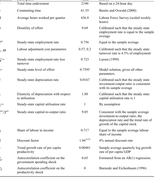
steady states, whereas consumption and capital move up more slowly. This is illustrated in Figure 1. Firms wish to exploit the temporary boost to productivity growth by increasing labour and capital services in production. But both employment (denoted by the variable Nbar) and the physical capital stock are predetermined at the time of the shock. Instead, firms operate along their intensive margins. The increased demand for capital and labour services is met by a temporary increase in utilisation and effort; higher investment contributes to meeting the increased demand for capital services in future periods. Unlike in Burnside and Eichenbaum (1996), effort remains persistently above its steady state level in the period following the shock, rather than immediately returning to zero. This is because we have assumed that there are costs to adjusting employment: workers are willing to supply higher levels of effort given that there are costs associated with changing the employment rate.

Figure 1: Productivity shock

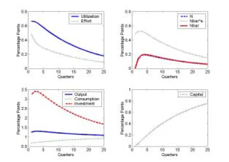
Following a temporary but persistent 1% government spending shock, Figure 2 shows that, on impact, investment is crowded out nearly one-for-one. However, output does increase somewhat, reflecting the temporarily higher level of aggregate demand. On impact, capital and labour services rise to meet this higher demand. Again, since both the capital stock and employment are predetermined, this must happen through increased effort and utilisation. In subsequent periods, because employment is costly to adjust, effort remains persistently above its steady state. The increase in utilisation raises the rate of depreciation and causes a temporary decline in the capital stock. The capital stock is eventually restored through temporarily higher investment in

Figure 2: Government spending shock

The above figures illustrate that capital utilisation and effort are a leading indicator of a firm’s decision to hire capital and labour, since by their very nature, utilisation rates can be adjusted more quickly than physical inputs such as the capital stock and employment. The responses also highlight the pro-cyclical nature of factor utilisation rates. Accounting for the behaviour of these unobservable inputs over the cycle is the objective of the next section.

4 Method

This section describes how we use the model in Section 2 to derive estimates for the unobservable variables of capital utilisation, labour effort, and total factor productivity. An expression for capital utilisation can be derived without recourse to the model solution by exploiting the fact that profit maximising firms equate the marginal productivity of capital utilisation (equation (18)) to its marginal cost, which itself is related to the marginal effect of utilisation on depreciation (equation (10)):(17)

(

)

1 1 1 t t t U K Y φ α δφ é ù − ê ú =_{ê ú} ê ú ë û (34)

Equation (34) shows that the capital-to-output ratio and utilisation are proportionally related in this model. Utilisation is high when the capital-to-output ratio is small, and vice-versa.

(17) _{As noted by Basu and Kimball (1997), optimising firms equate the marginal benefit of all factors to their}

Before we can derive an estimated series for utilisation, we need to construct a model-consistent measure of the capital-to-output ratio, i.e. one that takes into account time-varying depreciation. Given data on output and investment, and an assumption about the initial value of the capital-to-output ratio, the capital law of motion equation (6) together with equation (34), can be used to solve for the capital stock in a recursive fashion:(18)

1 1 1 1 t t t t t t t t K K I Y Y Y Y Y α φ + + + é − ù =_ê − + _ú ë û (35)

Using this series we can then obtain an estimate of utilisation using equation (34).

Calculating a series for labour effort and total factor productivity additionally requires data on total hours worked. However, not all variation in total hours worked comes from variations in the number of people employed (as our model assumes), since average hours worked vary too. To accommodate this, we re-express our labour adjustment cost specification (equation (3)) in terms of total hours, Ht,

(

)

2 1 2 2 t _{t t t} H H H H h h ω − æ ö =_ç − − + ∆ _÷ è ø, (36)

and then divide our total hours series by the population of working age to get series for Nt, the employment rate, and N_t, the effective employment rate:

h H N t t = (37) and h H N t t = . (38)

Variations in average hours observed in the data show up therefore as changes in the employment rate. Implicitly this assumes that adjustment costs are the same for average hours as they are for numbers employed (and indeed that employment in hours as well as heads is predetermined).(19) Given series for Ht and H_t, we are able to calculate labour effort (et) and total factor productivity (Xt) growth, which are pinned down by the production function and the model solution for effort. TFP growth is measured in the usual way as a residual from the production function:

1 1 1 1

1 1

1 1 1

log log log log

log log t t t t t t t t t _t t t X Y K U X Y K U e H e H α α α α α − − − − − ₋ æ ö₌ æ ö₋ − æ ö₋ − æ ö ç ÷ ç ÷ ç ÷ ç ÷ è ø è ø è ø è ø æ ö æ ö − _{ç ÷}− _{ç ÷} è ø è ø (39)

The growth rate of effort is related to the state and exogenous variables of the model:

(18) _{We choose an initial capital-to-output ratio that ensures the sample average of utilisation is equal to its}

steady-state level of 1.

(19) _{One could alternatively take the view that changes in average hours represent a change in the intensive margin as}

far as the firm is concerned, but the labour utilisation measure derived would conflate both changes in effort and changes in average hours. In any case, the broad message from series derived in this way is the same as that from the one we report.

(

)

0 1 2 1 1 1 1 4 3 4 1 1

log log log log

log log t t t t t t t t t t t t e H H K e H H K G X G X π π π π π π − − − − − − æ ö æ ö_{= +} æ ö₊ æ ö ç ÷ ç ÷ ç ÷ ç ÷ è ø è ø è ø è ø æ ö æ ö + _{ç ÷}+ − _{ç ÷} è ø è ø , ₍₄₀₎

where π_i is derived from the underlying model parameters.(20) The two equations can be solved simultaneously to generate two series for the growth rates of TFP and effort. By assuming an initial value for effort, we can back out the implied initial value for TFP from the production function (all of the other arguments are known) and calculate series for both effort and total factor productivity in levels.(21)

5 Estimated series for the United Kingdom(22)

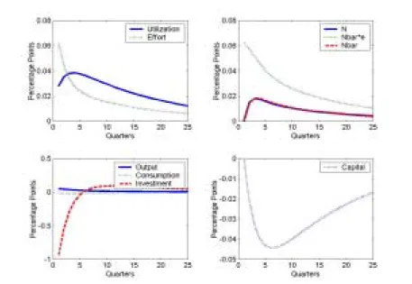
5.1 The capital-to-output ratio

Before reporting UK estimates for capital utilisation, effort, and TFP growth, we briefly discuss our estimated capital-to-output ratio series. Figure 3 contrasts our constructed series for the capital-to-output ratio based on time-varying depreciation (denoted ‘FU model’), with one based on an interpolation of official annual data on the capital stock.(23) Abstracting from differences in scale (the official data excludes housing capital), the counter-cyclical pattern in both series is the same. In particular, their similarity suggests that variable depreciation has a relatively small effect on the behaviour of the capital stock.(24) However, the recent divergence between the two measures reflects differences in the underlying rate of depreciation. Whereas our measure of the capital stock is derived under the assumption of cyclical variations in the rate of depreciation, the official measure allows for discrete changes in the depreciation rate arising from changes in the overall structure of the capital stock. For example, the implicit official depreciation rate has been increasing over the last decade as the share of short-lived of IT capital in the total capital stock has increased.(25)

(20) _{Using the calibrated parameter values as described in the previous section, we find that π}

0 = –0.4971, π1 =

–0.0131, π2 = –0.4923, π3 = 0.4923 and π4 = 0.0642.

(21) _{We choose an initial effort level that ensures the sample average for effort is equal to its steady-state value.} (22) _{A description of our data and its sources is given in the Appendix.}

(23) _{Annual observations on the capital stock are interpolated using investment data and a fixed depreciation rate.} (24) _{Basu and Kimball (1997) find this result for the US as well.}

Figure 3: Capital-to-output ratios 7.5 8.0 8.5 9.0 9.5 10.0 1965 1970 1975 1980 1985 1990 1995 2000 5.0 5.5 6.0 6.5 7.0 7.5

FU model (left-hand scale) Interpolated official data (right-hand scale)

5.2 Capital utilisation

Our series for capital utilisation is illustrated in Figure 4. As noted previously, fluctuations in our estimated series are negatively and proportionately related to contemporaneous changes in the capital-to-output ratio. The rise in the capital-to-output ratio since the late 1990s is therefore reflected in a decline in estimated capital utilisation over the same period.

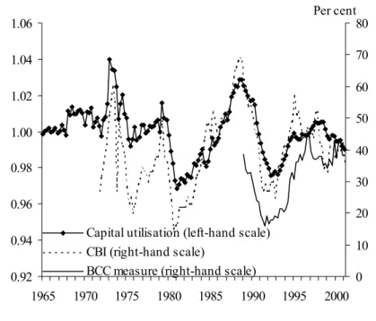
In order to evaluate our estimated series, we compare it to survey-based measures of capacity used by the Bank of England and others. Our constructed capital utilisation measure matches both the Confederation of British Industry (CBI) Industrial Trends Survey measure of capacity utilisation in manufacturing and a weighted average of the British Chambers of Commerce

(BCC) Quarterly Economic Survey’s manufacturing and services capacity measures quite well.(26) All three measures are strongly pro-cyclical, as one would expect. In particular, both the CBI measure and our estimate show utilisation peaking in the Lawson boom of the late 1980s before falling sharply. The strong positive correlation between our estimate of capital utilisation and both the CBI and BCC survey-based measures (0.69 and 0.56, respectively) provides supporting evidence that these measures capture the intensity with which firms utilise their capital stock.(27)

(26) _{Astley and Yates (1999) have also investigated the usefulness of the CBI measure in this context.}

Figure 4: Capital utilisation and survey-based measures 0.92 0.94 0.96 0.98 1.00 1.02 1.04 1.06 1965 1970 1975 1980 1985 1990 1995 2000 0 10 20 30 40 50 60 70 80

Capital utilisation (left-hand scale) CBI (right-hand scale)

BCC measure (right-hand scale)

Per cent

Measures of capital utilisation are often interpreted as having leading indicator properties, particularly for investment.(28) Shapiro (1989) investigates whether capacity utilisation, as an indicator of real activity, leads investment in the United States. The hypothesis is that high rates of capacity utilisation indicate that capacity is constrained, to which firms respond by investing to expand capacity in future periods. For three reasons, the model presented in Section 2 also predicts a leading relationship between capital utilisation and investment. First, if the shocks themselves are persistent, then high rates of utilisation may suggest high demand for capital services and therefore higher investment in future periods. Second, higher rates of utilisation are assumed to cause the capital stock to depreciate more quickly. Firms therefore need to increase investment in order to restore the capital stock to its long-run equilibrium following periods of relatively high capital utilisation. Finally, because employment takes time to adjust, and because employment and capital are complements in production, firms want any additions to the capital stock to become available at the same time as any increase in employment.

The strong link between investment and capital utilisation predicted by the model is illustrated in Figure 5. Given the close relationship between our estimate of utilisation and survey-based measures, this leading relationship is also evident between survey-based measures of capacity and investment, indicating the potential usefulness of such measures as an indicator of investment intentions, as often reported in the Bank of England’s Inflation Report.(29)

(28) _{Indeed, some of the questions regarding investment intentions in the CBI Quarterly Industrial Trends survey are}

linked specifically to capacity utilisation.

Figure 5: Capital utilisation and the investment-to-output ratio 0.96 0.97 0.98 0.99 1.00 1.01 1.02 1.03 1.04 1.05 1965 1970 1975 1980 1985 1990 1995 2000 0.16 0.17 0.18 0.19 0.20 0.21 0.22 0.23 Capital utilisation (left-hand scale)

I/Y ratio (right-hand scale)

5.3 Labour effort

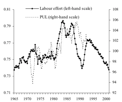
Our estimated effort series for the UK is illustrated in Figure 6. Unlike capital utilisation, there are no up-to-date survey measures of labour effort against which to compare our series.(30)

However, from the early 1970s to the early 1990s, Bennett and Smith-Gavine (1987, 1997) derive a series known as the Percentage Utilisation of Labour (PUL). The PUL is based on monthly responses from plants in which production managers provide work-study based information on the intensity of utilisation of operatives. Although largely a subjective measure, and one confined solely to the manufacturing sector, it attempts to strip out the effects of technical change, capital deepening and hours of work, from labour productivity.(31) In principle, therefore, it should be similar to our estimated series for effort. The two track each quite well until the late 1980s, when our derived effort series starts to fall about eighteen months before the PUL. Consequently the correlation between our estimated effort series and the PUL, although positive, is somewhat low, at 0.51. Part of this low correlation may be an artefact of the deterioration in the final years of its construction of the sample on which the PUL was based. Changes in work practices meant that many firms no longer collected the source data for the PUL as a matter of course, and the non-response rate consequently increased (Bennett and Smith Gavine, 1997, pages 12-13). Indeed if we exclude this period, the correlation between our effort series and the PUL rises to 0.74.

(30) _{Though employee surveys indicate effort increased over the 1990s in the UK (see Green, 2001).}

Figure 6: Effort and the Percentage Utilisation of Labour 0.71 0.73 0.75 0.77 0.79 0.81 1965 1970 1975 1980 1985 1990 1995 2000 92 94 96 98 100 102 104 106 108

Labour effort (left-hand scale) PUL (right-hand scale)

Figure 7: Effort and total hours worked

0.71 0.72 0.73 0.74 0.75 0.76 0.77 0.78 0.79 0.80 0.81 0.82 1965 1970 1975 1980 1985 1990 1995 2000 300 310 320 330 340 350 360

Labour effort (left-hand scale)

Total hours per capita (right-hand scale)

Although effort is a function of several variables, it is most strongly influenced by fluctuations in total hours.(32) The two series are highly negatively correlated (−0.89), as predicted by the model and illustrated in Figure 7. The substitution between total hours and effort is quite intuitive in our model: as a boom is in its initial stages, firms demand an increase in labour effort in order to (32) _{This is evident from the size of the coefficient on total hours in the model solution for effort reported in footnote}

generate labour services. Thereafter, firms satisfy their demand for increased labour services by increasing employment with effort slowly returning to its steady state. Since the mid-1990s, our estimates indicate that effort levels have been declining, reflecting the rise in total hours per capita. However, the persistent nature of the rise in total hours worked suggests it may be

structural rather than a response to shocks. Our model – which has balanced growth and only one sector – assumes that hours worked is a stationary stochastic process and therefore cannot

properly account either for persistent movements in hours or for any structural change.(33) Consequently the decline in our estimated effort series may well be overstated.

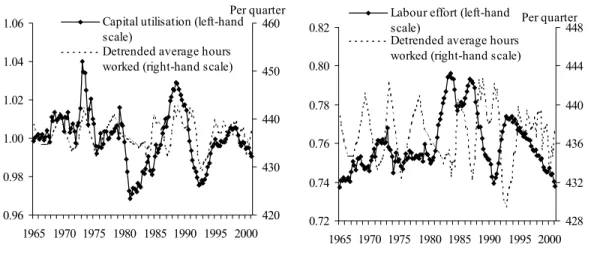
5.4 Intensive margins

Basu and Kimball (1997) suggest that, since firms wish to exploit all their intensive margins (utilisation, effort, and average hours) to the same extent, movements in average hours (which are directly observable) should provide sufficient information about movements in other margins. Figure 8a and Figure 8b compare average hours worked per quarter against utilisation and effort.

Figure 8a and Figure 8b: Measures of intensive margins

0.96 0.98 1.00 1.02 1.04 1.06 1965 1970 1975 1980 1985 1990 1995 2000 420 430 440 450 460 Capital utilisation (left-hand scale)

Detrended average hours worked (right-hand scale)

Per quarter 0.72 0.74 0.76 0.78 0.80 0.82 1965 1970 1975 1980 1985 1990 1995 2000 428 432 436 440 444 448 Labour effort (left-hand

scale)

Detrended average hours worked (right-hand scale)

Per quarter

Utilisation and average hours track each other reasonably well, except for a period in the early 1980s (the full sample correlation is 0.53). The relationship between labour effort and average hours is somewhat puzzling. At the beginning and end of the sample period, the relationship appears to be positive, as expected. During the 1980s and early 1990s, however, the relationship appears strongly negative. Indeed, the correlation between the two series is –0.28 over the sample. By contrast, the PUL measure is positively correlated with average hours over a shorter sample period, although still somewhat low at 0.27.

(33) _{Indeed we cannot reject the hypothesis of a unit root in our series on total hours. Chang and Kwark (2001) find a}

5.5 Total factor productivity

Given data on output and employment, and our estimated series for the capital stock, capital utilisation and labour effort, we can back out a series for total factor productivity growth (TFP) using the production function (see equation (39)). Figure 9 compares our series to growth in an hours-based estimate of the Solow residual, a standard proxy for TFP.(34) Our measure of annual TFP growth still display marked peaks and troughs consistent with the economic cycle, though by accounting for variations in factor utilisation, the standard deviation of TFP growth is reduced by 50%. This is due to the cyclical nature of factor utilisation, which is not accounted for in

traditional Solow residual estimates of TFP.

Figure 9: Annual growth in total factor productivity

-10 -5 0 5 10 15 1965 1970 1975 1980 1985 1990 1995 2000 FU model Solow residual Per cent

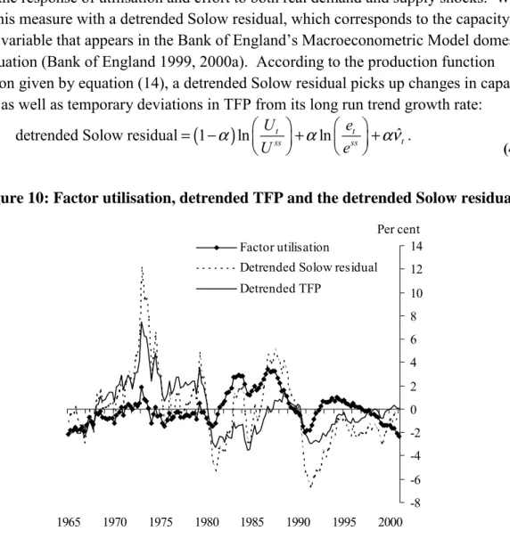
5.6 Aggregate factor utilisation

Economy wide measures of capacity utilisation are often used as indicators of excess demand and firm pricing pressures.(35) We derive a measure of aggregate factor utilisation from our estimated capital utilisation and effort series. This measure, denoted FU, weights together our utilisation and effort series (expressed relative to their steady state values):

(

)

÷ ø ö ç è æ + ÷ ø ö ç è æ − = _sst ss t t _e e U U FU 1 α ln αln . ₍₄₁₎ (34) _{This Solow residual is derived using total hours worked and the interpolated official capital stock data as its factor}

inputs.

(35) _{See Blanchard and Fischer (1989) p. 464 for early references, Stock and Watson (1999), Gordon (1998), and}

It reflects the response of utilisation and effort to both real demand and supply shocks. We compare this measure with a detrended Solow residual, which corresponds to the capacity utilisation variable that appears in the Bank of England’s Macroeconometric Model domestic pricing equation (Bank of England 1999, 2000a). According to the production function specification given by equation (14), a detrended Solow residual picks up changes in capacity utilisation as well as temporary deviations in TFP from its long run trend growth rate:

(

)

ˆ

detrended Solow residual 1 ln t ln t

t ss ss U e U e α æ ö α æ ö αν = − _{ç ÷}+ _{ç ÷}+ è ø è ø . (42)

Figure 10: Factor utilisation, detrended TFP and the detrended Solow residual

-8 -6 -4 -2 0 2 4 6 8 10 12 14 1965 1970 1975 1980 1985 1990 1995 2000 Factor utilisation

Detrended Solow residual Detrended TFP

Per cent

Figure 10 shows that our estimate of factor utilisation and the detrended Solow residual have not moved that closely over the sample period (the correlation coefficient is 0.40). Indeed, our estimate of TFP accounts for movements in the Solow residual to a much greater extent: the correlation between them is 0.83. It is not surprising that, as a measure of excess demand pressure, estimates of capacity utilisation that include temporary shocks to TFP may be

misleading, particularly in periods where TFP deviates significantly from its trend growth rate. In fact, as Figure 11 demonstrates, our measure of aggregate factor utilisation corresponds much more closely to detrended labour productivity (output per hour) than to the detrended Solow residual (the correlation coefficient is 0.73). In some ways this is not surprising: if capital and labour are slow to adjust, then much of the variation in factor inputs – and hence output – over the cycle must come from utilisation and effort. Some authors (Roberts, 2001, for example) have interpreted the cyclicality of output per hour as indicating that the average productivity of labour deviates from the marginal productivity, perhaps because of labour hoarding. A productivity measure defined as output per unit of effective labour input

(

Y He

)

may be a better measure of the marginal cost of labour, and may therefore be less cyclical than a simple output per hour measure. Figure 12 shows that this does seem to be the case: the standard deviation of annual

labour productivity growth is reduced by almost 40% if one uses a measure of effective labour input.

Figure 11: Factor utilisation and detrended labour productivity

-6 -4 -2 0 2 4 6 8 1965 1970 1975 1980 1985 1990 1995 2000 Factor utilisation

Detrended labour productivity Per cent

Figure 12: Measures of annual labour productivity growth

-6 -4 -2 0 2 4 6 8 10 1965 1970 1975 1980 1985 1990 1995 2000 Per cent Output per effective labour input Output per hour

5.7 Accounting for changes in our derived series

As an expositional device, we examine the relative contributions that observable data (output, employment, government expenditure and the capital stock) make to changes in our estimated series (capital utilisation, labour effort, total factor productivity and aggregate factor utilisation). Though not necessarily meaningful in terms of causality, such an exercise can be a helpful in giving some intuition for – and perhaps a plausibility check on – the profiles we derive. Figure 13 shows the contributions to annual growth rates of our estimated series.(36)

Our derived capital utilisation series is inversely proportional to the capital-to-output ratio (equation (34)) and as such movements in this variable can be completely accounted for by movements in output and the capital stock. The capital stock is relatively slow to adjust: it is not surprising therefore that most of the short-term fluctuations in utilisation are accounted for by changes in output. In accordance with the model solution for labour effort growth (equation (40)), much of the fluctuations in effort are due to fluctuations in employment: the steady increase in employment since 1993 is the principal reason that labour effort has been declining over this period. Using the solutions for utilisation and effort, together with the production function (equation (39)), we can also back out the contributions observable data make to our series for TFP growth. Not surprisingly, given that our productivity series is still quite pro-cyclical, movements in output and employment account for most of the movement in TFP. The same is true for our aggregate factor utilisation measure, which we would expect given its correlation with detrended output per hour.

(36) _{Note that variables that grow over time (output, government expenditure, TFP and the capital stock) have been}

33

Figure 13: Accounting for annual growth in labour effort, capital utilisation, TFP and aggregate factor utilisation

-4.0 -3.0 -2.0 -1.0 0.0 1.0 2.0 3.0 4.0 1966 1971 1976 1981 1986 1991 1996 Govt. contribution Capital contribution Employment contribution Output contribution Labour effort growth

Labour effort growth Percent

-5.0 -4.0 -3.0 -2.0 -1.0 0.0 1.0 2.0 3.0 4.0 5.0 6.0 1966 1971 1976 1981 1986 1991 1996 Government contribution Capital contribution Employment contribution Output contribution Productivity growth

Productivity growth Percent

-3.0 -2.0 -1.0 0.0 1.0 2.0 3.0 4.0 1966 1971 1976 1981 1986 1991 1996 Output contribution Capital contribution Capital utilisation growth

Capital utilisation growth Percent

-3.0 -2.0 -1.0 0.0 1.0 2.0 3.0 1966 1971 1976 1981 1986 1991 1996

Output contribution Employment contribution Capital contribution Govt. contribution Factor utilisation growth

6 Conclusion

We investigate a general equilibrium model (based on Burnside and Eichenbaum, 1996) with time-varying factor utilisation and labour adjustment costs. Our findings show firms initially respond to unanticipated shocks by altering factor utilisation rates. In subsequent periods, they adjust

observable inputs such as physical capital and employment. As a result, utilisation rates are a leading indicator of firms’ hiring of capital and labour.

Our focus is mainly on the estimated series of factor utilisation and TFP for the UK. We find that our estimate of capital utilisation tracks survey-based measures quite closely, providing supporting evidence that these measures do indeed capture the extent to which firms are utilising their existing capital stock. Given the strong relationship between investment and utilisation as predicted by the model, this finding indicates the potential usefulness of the surveys for the purposes of forecasting investment.

Movements in total hours worked drive our estimate of labour effort. As a consequence, the recent declines in labour effort are attributable to the strength of total hours worked. If the rise in total hours is due to structural changes, which our model does not account for, then the estimated declines in effort are most likely overstated. We compare our estimate of labour effort to a corresponding survey measure, as well as to movements in average hours. Contrary to theoretical predictions, the relationship between them is fairly low, indicating a potential weakness in the model in disaggregating between the various inputs in effective labour.

Our estimate of TFP growth is found to be less cyclical than the rate of growth of a traditional Solow residual. Nevertheless, a weighted average of capital utilisation and labour effort –

aggregate factor utilisation – and the detrended Solow residual are not closely related, suggesting that measures which conflate both capacity utilisation and temporary deviations in TFP from its steady-state growth rate may be misleading indicators of excess demand pressure.

Rather, our measure of aggregate factor utilisation is correlated with detrended labour productivity, providing more evidence that differences in average and marginal labour productivity may be linked to factor hoarding. Labour productivity calculated as output per unit of effective labour input is less cyclical than a simple output per hour measure.

35 Appendix

Table B: Correlation Matrix

Observable variables Derived variables Memo items

D etr ende d o utput Inve stm ent-out put r atio Em ploym en t r ate Tota l h our s pe r cap ita Av erag e h ou rs D etr ende d la bour pr oduc tivity D etr ende d S olow re sidua l Ca pita l-ou tp ut ra tio Ca_pita l utilisa tio n La bour e ffo rt D etr ende d eff ec tive la bour pr oduc tivity . Fa ctor uti lisa tio n D etr ende d TF P CBI BCC PU L Standard Deviation (%) 3.52 6.97 3.25 3.46 0.63 2.29 3.15 2.66 1.41 1.93 1.79 1.34 2.13 30.20 28.13 2.77

Observable variables Correlation

Detrended output 1 0.38 0.77 0.79 0.37 0.33 0.73 -0.82 0.82 -0.49 0.88 -0.25 0.93 0.23 0.61 -0.40

Investment-output ratio 0.38 1 0.55 0.57 0.25 -0.28 0.10 -0.52 0.52 -0.53 0.18 -0.39 0.27 0.40 0.46 0.09

Employment rate 0.77 0.55 1 0.98 0.26 -0.32 0.23 -0.56 0.55 -0.90 0.46 -0.76 0.51 0.01 0.38 -0.49

Total hours per capita 0.79 0.57 0.98 1 0.43 -0.32 0.25 -0.62 0.61 -0.89 0.46 -0.73 0.53 0.11 0.41 -0.41

Average hours 0.37 0.25 0.26 0.43 1 -0.09 0.18 -0.53 0.53 -0.28 0.17 -0.13 0.26 0.49 0.38 0.27

Detrended labour productivity 0.33 -0.28 -0.32 -0.32 -0.09 1 0.76 -0.31 0.32 0.62 0.65 0.73 0.62 0.23 0.09 -0.05

Detrended Solow residual 0.73 0.10 0.23 0.25 0.18 0.76 1 -0.76 0.76 0.17 0.78 0.40 0.83 0.46 0.66 -0.03

Derived variables

Capital-output ratio -0.82 -0.52 -0.56 -0.62 -0.53 -0.31 -0.76 1 -1.00 0.25 -0.62 -0.05 -0.75 -0.69 -0.57 -0.11

Capital utilisation 0.82 0.52 0.55 0.61 0.53 0.32 0.76 -1.00 1 -0.24 0.62 0.06 0.75 0.69 0.56 0.12

Labour effort -0.49 -0.53 -0.90 -0.89 -0.28 0.62 0.17 0.25 -0.24 1 -0.19 0.96 -0.22 0.18 -0.31 0.51

Detrended effective labour

productivity 0.88 0.18 0.46 0.46 0.17 0.65 0.78 -0.62 0.62 -0.19 1 -0.01 0.98 0.09 0.72 -0.50

Factor utilisation -0.25 -0.39 -0.76 -0.73 -0.13 0.73 0.40 -0.05 0.06 0.96 -0.01 1 0.00 0.41 -0.13 0.56

Detrended total factor productivity 0.93 0.27 0.51 0.53 0.26 0.62 0.83 -0.75 0.75 -0.22 0.98 0.00 1 0.24 0.76 -0.39

Memo items

CBI 0.23 0.40 0.01 0.11 0.49 0.23 0.46 -0.69 0.69 0.18 0.09 0.41 0.24 1 0.55 0.62

BCC 0.61 0.46 0.38 0.41 0.38 0.09 0.66 -0.57 0.56 -0.31 0.72 -0.13 0.76 0.55 1 0.76